On Stability of Hawkes Process

Abstract

Existence and stability properties are studied for Hawkes process, i.e. point process $S$ that has long-memory and intensity $r(t)=\lambda\big{(}g_{0}(t)+\sum_{\tau<t,\tau\in S}h(t-\tau)\big{)}$. The approach to Hawkes process presented in this paper allows us to prove the uniqueness of invariant distribution of the process under weaker conditions. New speed of convergence results are also shown. Unlike previous results the function $\lambda$ is not required to be Lipschitz and can be even discontinuous. Some generalizations are also considered.

arXiv:1201.1573

t11Partially supported by NSF grants:DMS-0904701, DMS-1208334 and DARPA.

1 Introduction

1.1 Definition

Hawkes Process is a time-homogeneous self-exciting locally-finite point process on ${\mathbb{R}}$ with long-memory. A realization of the process is a random locally-finite subset $S=S(\omega)$ of ${\mathbb{R}}$. Any locally-finite point process is characterized by its intensity rate $r(t,\omega)$ defined as the intensity of the point process at time $t$ conditioned on the past history of the process until time $t$, i.e. $r(t,\omega)$ can be defined as

$$r(t,\omega):=\lim_{\delta t\to 0}\frac{{\mathbb{P}}\bigg{[}\#\big{(}S(\omega)\cap[t,t+\delta t)\big{)}\geq 1|{\mathcal{F}}_{t}\bigg{]}}{\delta t}$$ (1)

where $\#\big{(}S(\omega)\cap[t,t+\delta t)\big{)}$ is the number of elements of the set $S(\omega)\cap[t,t+\delta t)$ and ${\mathcal{F}}_{t}$ is the $\sigma-$field for $S_{t}(\omega):=S(\omega)\cap(-\infty,t)$ generated by elementary events $\{\omega:S_{t}(\omega)\cap I\neq\emptyset\}$ where $I$ varies over all intervals $I\subset(-\infty,t)$.

It is convenient to view the process as a random subset of ${\mathbb{R}_{+}}:=[0,\infty)$ and thus the intensity function $r(t,\omega)$ is defined for $t\in{\mathbb{R}_{+}}$. Hawkes Process is defined by three ${\mathbb{R}_{+}}$-valued functions on ${\mathbb{R}_{+}}$. Given these three functions $\lambda,h,g_{0}$ the intensity rate is given by

$$r(t,\omega)=\lambda\big{(}g_{0}(t)+\sum_{\tau\in S_{t}}h(t-\tau)\big{)}$$ (2)

where $g_{0}$ is some initial condition.

The above description is equivalent to the one found in literature except for the term $g_{0}$. Usually instead of starting from initial condition $g_{0}$, the process is defined by giving $S_{0}$ a locally finite collection of points in $(-\infty,0)$. This set $S_{0}$ represents points of process before time $0$. To connect to our setting $g_{0}$ can then be computed as

$$g_{0}(t)=\sum_{\tau\in S_{0}}h(t-\tau)$$ (3)

and the the two definitions are equivalent. Defining process with $g_{0}$ as initial conditions also allow for more general functions which are not of form (3).

This approach, besides providing this slight generalization of the model, leads to a somewhat different perspective: Hawkes process is a solution of a stochastic partial differential equation with jumps. In fact Hawkes process corresponds to solution of one of the simplest such equations where the state of the process at time $t$ is the random impulse function $g_{t}(\cdot)$ that evolves by translation in time $g_{t+\delta t}(\cdot)=g_{t}(\cdot+\delta t)$ with jumps $g_{t}(\cdot)\to g_{t}(\cdot)+h(\cdot)$ occurring at rate $\lambda(g_{t}(0))$. There is a built-in invariance under time translation due to the form of (2). The evolution of the impulse function $g_{t}:{\mathbb{R}_{+}}\to{\mathbb{R}_{+}}$ is defined by:

$$g_{t}(s)=g_{0}(t+s)+\sum_{\tau\in S_{t}}h(t+s-\tau)$$ (4)

It is ${\mathcal{F}}_{t}$-measurable and is a Markov process (it need not contain all the past information as is the case when $h(t)=e^{-t}$). Given two times $s\geq t\geq 0$, the conditional distribution of the next $\tau\in S$ after time $t$ being greater than $s$ is given by

$${\mathbb{P}}[\tau\geq s|{\mathcal{F}}_{t}] := {\mathbb{P}}\big{[}S\cap[s,t)=\emptyset,S\cap[t,\infty)\neq\emptyset|{\mathcal{F}}_{t}\big{]}$$ (5)

$$= \exp\left[-\int_{0}^{s-t}\lambda(g_{t}(s))ds\right]$$ (6)

at which point $g_{\tau}(\cdot)$ jumps to $g_{\tau}(\cdot)+h(\cdot)$. Thus $g_{t}$ is by itself a Markov process.

1.2 Results

The two main results of this paper, Theorems 2 and 3, generalize the results of Brémaud-Massoulié [1] in different directions and prove that under certain conditions on $\lambda$ and $h$, for a certain wide class $\mathcal{C}$ of initial conditions $g_{0}$, the distributions of $g_{t}(\cdot)$ converge to a common limit. Furthermore the limiting distribution is supported on $\mathcal{C}$. The secondary new result, Theorem 4, is on speed of convergence.

In addition to these theorems we also observe several facts well known for attractive systems. These are collected in Proposition 1. The results are stated in sections 4 and 5.

1.3 History and references to related work

Point processes were first studied in [4] by Erlang in connection with queueing theory. Hawkes process were first introduced in [5] to study self-exciting point processes. See [2, 3] for additional references. The current work is the first one that covers cases where $\lambda$ need not be Lipschitz and in fact can even have jumps. Large deviations questions for wide classes of $\lambda$ and $h$ have been studied by Zhu in [9] and [10]; for the special case of linear $\lambda$ explicit large deviation rates and other limit theorems have been derived in [7].

Currently Hawkes processes are used to model many phenomena ranging from queues and population growth to mutations and spread of infections; to defaults and jumps in financial markets; to neuroactivity and social-networks; and finally even to modeling of artificial intelligence and creative thinking. While most of the real world applications involve use of multi-dimensional Hawkes process, in order to keep the presentation simple, we limit ourselves to the one-dimensional version. Possible generalizations are outlined in section 7.

1.4 Example

Simple example comes from population growth. Consider a population that grows either by immigration or by birth generated by the current population. Immigrants are treated as newborns when they arrive. The immigration rate is $A$ and the birth rate for each individual is $h(s)$, which depends only on the current age $s$ of the individual. Then total growth rate of the population at time $t$ is then given by

$$r(t)=A+\sum_{\tau\in S,\tau<t}h(t-\tau)$$ (7)

or if we normalize with $h$ by $\int_{0}^{\infty}h(s)ds=1$, we replace this by

$$r(t)=A+B\sum_{\tau\in S,\tau<t}h(t-\tau)$$ (8)

since $B$ comes out of normalization. So we see that this is a Hawkes process with $\lambda(z)=A+Bz$. The Hawkes processes with such linear $\lambda$ appear very often and are related to Galton-Watson trees which in turn provides an easy way of studying many properties of Hawkes processes.

2 Formal Definitions

2.1 Formal Definition of a Hawkes Process

Definition 1.

Hawkes process is a random collection $S$ of points in ${\mathbb{R}_{+}}:=[0,\infty)$ characterized by triplet of functions $(\lambda,h,g_{0})$ where the functions $\lambda,h,g_{0}:[0,\infty)\to[0,\infty)$. The conditional Poisson intensity at time $t$ is

$$r_{t}:=\lambda\left(g_{0}(t)+\sum_{0\leq\tau<t,\tau\in S}h(t-\tau)\right)$$ (9)

where the sum is over all previous points $\tau$ in $S_{t}:=S\cap[0,t)$. The function $g_{0}$ describes the initial condition and the functions $\lambda$ and $h$ describe the evolution of the process. We denote this Hawkes process by quadruple $({\mathbb{P}},\lambda,h,g)$.

We will define a coupling of these different measures ${\mathbb{P}}_{g}$ by a canonical construction in the subsection 3.1.

It is convenient to take as state space the space ${X}$ of locally integrable ${\mathbb{R}_{+}}$-valued functions on ${\mathbb{R}_{+}}$. Let ${\mathcal{M}}(X)$ be the space of probability distributions on ${X}$. Then the process can be realized as an ${X}$-valued process. Start at time $t$ from with initial condition $g_{t}\in{X}$ and consider the random evolution determined by two components: deterministic flow $g_{t+\delta t}(s)=g_{0}(t+\delta t+s)$ up to stopping time $\tau$ at which point $g_{\tau}$ jumps $g_{\tau+0}(x)=g_{\tau-0}(x)+h(x)$ with the distribution of $\tau=\tau(g)$ given by

$${\mathbb{P}}_{g}[\tau\geq t+\delta t]=\exp\left[-\int_{0}^{\delta t}\lambda(g_{t}(s))ds\right].$$ (10)

After time $\tau$, the process restarts in the sense that same procedure is to be repeated with $\tau$ as a new starting time and $g_{\tau}$ as a new initial condition. Each time stopping corresponds to a point in $S$. The generator of the semi-group $T_{t}$ of the Markov process acting on functions $F:{X}\to{\mathbb{R}_{+}}$ is given by:

$$\mathcal{A}:=\mathcal{D}+\lambda(g(0))(\theta_{h}-\mbox{Id})$$ (11)

where $\theta_{h}$ is a shift operator defined by $(\theta_{h})F(g)=F(g+h)$ and $\mathcal{D}$ is the derivative of push-forward of time evolution defined by

$$\mathcal{D}F(g):=\lim_{\epsilon\to 0}\frac{F(\sigma_{\epsilon}g)-F(g)}{\epsilon}$$ (12)

where $\sigma_{\epsilon}$ is the time-shift operator defined by $\sigma_{\epsilon}g(s)=g(s+\epsilon)$. Then this ${X}$-valued process $g_{t}$ satisfies

$$g_{t}(s)=g_{0}(t+s)+\sum_{\tau\in S_{t}}h(t+s-\tau).$$ (13)

For any initial condition $g_{0}(\cdot)$, we have a Markov process $g_{t}(\cdot)$. Then $\lambda(z_{t})$ will be the intensity of the point process, where

$$z_{t}:=g_{t}(0)=g_{0}(t)+\sum_{\tau\in S_{t}}h(\tau-t).$$ (14)

It is sometimes more convenient to consider instead of $S_{t}$ the process

$$Q_{t}=(N_{t},g_{t})$$ (15)

where $N_{t}=\#(S_{t})$ is the number of jumps from time $0$ to time $t$. Then $Q_{t}$ can be viewed as a point process $N_{t}$ driven by the Markov process $g_{t}$.

Remark 1.

Without loss of generality we can assume $\int_{0}^{\infty}h(t)dt=1.$ Indeed one can always achieve this if $\|h\|_{1}=\int h(t)dt<\infty$ by observing that triples $\big{(}\lambda(z),h(t),g(t)\big{)}$ and $\left(\lambda(z\|h\|_{1}),\frac{h(t)}{\|h\|_{1}},\frac{g(t)}{\|h\|_{1}}\right)$ produce the same Hawkes process. On the other hand if $\|h\|_{1}=\infty$ and $\inf_{z\in{\mathbb{R}_{+}}}\lambda(z)>0$ then $\lim_{t\to\infty}g_{t}(0)=\infty$ a.s. and hence there can be no stationary version of the process.

2.2 Convergence notions

We equip the space $X$ with $L_{1}^{loc}$ metric

$$\forall g,f\in X,\qquad d_{X}(g,f)=\sum_{i=1}\frac{1}{2^{n}}\cdot\frac{\int_{0}^{n}|g(s)-f(s)|ds}{1+\int_{0}^{n}|g(s)-f(s)|ds}$$ (16)

The space ${\mathcal{M}}(X)$ will then have the topology of weak convergence inherited from the metric space $X$. Let $D(X)$ be the space of $X$-valued functions on $[0,\infty)$ equipped with Skorohod $J_{1}$-metric $d$ and let ${\mathcal{G}}$ be the $\sigma$-field generated by the open sets in $({X},d)$. Collection $\{{\mathcal{G}}_{t}\}$ is the corresponding filtration. Let $g^{*}$ be the non-initial part of impulse function:

$$g_{t}^{*}(s)=\sum_{\tau\in S_{t}}h(t+s-\tau)$$ (17)

and

$$\forall g,\widetilde{g}\in D(X),\qquad d^{*}(g,\widetilde{g}):=d(\mathcal{S}(g),\mathcal{S}(\widetilde{g}))=d(g^{*},\widetilde{g}^{*})$$ (18)

be the pull-back of $d$ under the map $\mathcal{S}:D(X)\to D(X)$, $\mathcal{S}:g\mapsto g^{*}$ defined according to (17) as

$$\big{(}\mathcal{S}(g)\big{)}_{t}(s)=g_{t}(s)-g_{0}(t+s)$$ (19)

Let $\mu_{f,s}$ be the distribution of $g_{s}$—impulse-function at time $s$—starting from initial condition $f$.

The distribution of the whole process $g$ starting with initial condition $g_{0}$ will be denoted by ${\mathbb{P}}_{g_{0}}$ and the associated expectations will be denoted by ${\mathbb{E}}_{g_{0}}$. Any $\mu\in{\mathcal{M}}(X)$ can be viewed as a random initial condition and

$${\mathbb{P}}_{\mu}:=\int{\mathbb{P}}_{f}\mu(df),\quad{\mathbb{E}}_{\mu}:=\int{\mathbb{E}}_{f}\mu(df),$$ (20)

denote the corresponding probability measure and expectation with respect to it. Similarly ${\mathbb{P}}^{*}$ and ${\mathbb{E}}^{*}$ will be used as analogous expressions for the $g^{*}$.

In Theorems 2 and 3 we consider total variation $d_{TV}$ of the difference of ${\mathbb{P}}^{*}$ starting from two different initial conditions which can also be viewed as total variation of the corresponding ${\mathbb{P}}$ but under a different $\sigma$-field ${\mathcal{G}}^{*}={\mathcal{G}}\circ\mathcal{S}^{-1}$.

Furthermore let us define $d_{TV,T}$ to be the total variation after time $T$, i.e. the total variation on the sigma-algebra ${\mathcal{G}}\circ\big{(}S|_{[T,\infty)}\big{)}^{-1}$ where operator $(S|_{[T,\infty})$ is defined by:

$$\big{(}\mathcal{S}|_{[T,\infty)}(g)\big{)}_{t}(s)=1_{t>T}\big{(}g_{t}(s)-g_{0}(t+s)\big{)}$$ (21)

3 Tools

3.1 Canonical Construction

One way to construct point processes is to start from a canonical Poisson point process ${\mathbb{P}}$. To any measure $m$ one can associate a Poisson point process such that for any measurable set $A$, the number of points in $A$ will be random variable with a Poisson distribution with mean $m(A)$. In our case canonical Poisson point process will correspond to the choice $m(A)=|A|$, the Lebesgue measure on ${\mathbb{R}_{+}}\times{\mathbb{R}_{+}}$. Given $\lambda,h,g$ measure ${\mathbb{P}}$ induces a measure ${\mathbb{P}}_{g}^{\lambda,h}$ consistent with the definition above in the following way. If $S$ is our point process then $\tau\in S$ if there is a point on the vertical line ${\tau}\times[0,\lambda(z_{t}))$ of our plane ${\mathbb{R}_{+}}\times{\mathbb{R}_{+}}$. In the rest of the paper we will denote ${\mathbb{P}}_{g}^{\lambda,h}$ by ${\mathbb{P}}_{g}$ because $\lambda$ and $h$ would be the same unless stated otherwise.

This induces a natural coupling of the collection of the measures $({\mathbb{P}}_{g})$ indexed by initial conditions $g$ that we will call canonical coupling. This coupling is no way unique but this particular coupling is maximal when $\lambda$ is non-decreasing and we have two different initial conditions one of which is strictly larger than the other (by point-wise partial ordering). The coupling is maximal in the sense that the set of points common to both of these two processes will stochastically dominate the similar set of points in any other coupling.

3.2 Coupling / Stochastic Domination

Here we present the canonical coupling that we will use.

Lemma (Stochastic Domination).

Suppose $(S,\lambda,h,g_{0})$ and $(\widetilde{S},\widetilde{\lambda},\widetilde{h},\widetilde{g}_{0})$ are two Hawkes processes satisfying

$$\forall x\in{\mathbb{R}_{+}},(h(x)\leq\widetilde{h}(x),g(x)\leq\widetilde{g}(x))$$ (22)

$$\forall x\leq y,\lambda(x)\leq\widetilde{\lambda}(y)$$ (23)

Then there exists a coupling such that $S{\subset}\widetilde{S}$.
Note: $h,\widetilde{h}$ are not necessarily normalized.

Proof.

If $a(t)$, $b(t)$ are two intensities and if $a(t)\leq b(t)$ for all $t$, one can couple the point processes, such that the two processes jump together with rate $a(t)$ and the second one jumps by itself at rate $b(t)-a(t)$. This can also be done if $\forall\omega\in\Omega,a(t,\omega)\leq b(t,\omega)$. (In fact this is done naturally by our construction that is discussed in the previous subsection.) Hence it remains to prove that

$$\lambda(g_{t}(0))\leq\widetilde{\lambda}(\widetilde{g}_{t}(0)).$$ (24)

We know that up to the first jump in $\widetilde{S}$ we have $g_{t}(0)=g_{0}(t),\widetilde{g}_{t}(0)=\widetilde{g}_{0}(t)$. However we know from (22) and (23) that

$$\lambda(g_{0}(t))\leq\widetilde{\lambda}(\widetilde{g}_{0}(t))$$ (25)

which in turn implies that (24) holds up to first jump of $\widetilde{S}$. Then we claim by induction that it holds for all times. Indeed at the time of jump the order of $g\leq\widetilde{g}$ is preserved because there is no jump in $S$ before first jump of $\widetilde{S}$ and the jump of $\widetilde{g}$ is always larger because $h\leq\widetilde{h}$. ∎

3.3 Parent-Offspring Structure and the Branching representation

We add the following parent-offspring structure to obtain a random forest structure embedded in time. This will be useful due to its connection to Galton-Watson trees (branching processes).

We start with the Hawkes process corresponding to functions $(\lambda,h,g_{0})$ and let $S=\{\tau_{1},\tau_{2},...\}$, where $\tau$ is an increasing sequence, i.e. $i<j\rightarrow\tau_{i}<\tau_{j}$. Let us also denote

$$\lambda_{0}(z):=\lambda(z)-\lambda(0)$$ (26)

Now to each $\tau_{i}$ we associate a randomly chosen parent element $p(\tau_{i})$ from $S\cup\{-\infty\}$, where $-\infty$ represents having no parent and being a root node. Given a sequence $(\tau_{1},\tau_{2},...,\tau_{i})$, we define $\{p(\tau_{i})\}$ to be mutually independent with distributions given by :

$${\mathbb{P}}[p(\tau_{i})=-\infty|\tau_{1},...\tau_{i}] = \frac{\lambda(0)}{\lambda(z_{\tau_{i}})}+\frac{\lambda_{0}(z_{\tau_{i}})}{\lambda(z_{\tau_{i}})}\frac{g(\tau_{i})}{z_{\tau_{i}}}$$ (27)

$${\mathbb{P}}[p(\tau_{i})=\tau_{j}|\tau_{1},...\tau_{i}] = 1_{j<i}\frac{\lambda_{0}(z_{\tau_{i}})}{\lambda(z_{\tau_{i}})}\frac{h(\tau_{i}-\tau_{j})}{z_{\tau_{i}}}$$ (28)

Note that $\{p(\tau_{i})\}$ while mutually independent are not identically distributed.

Figure 1 provides a particular visualization of parent-offspring structure that is consistent with the above description.

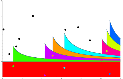
Figure 1: For both $\lambda(z)=1+z,\quad h(t)=\frac{1}{(1+t)^{2}}$. Each region corresponds to children of point of corresponding color

We are specifically interested in linear case which provides us with dual description of the same process as described in the following tool:

Lemma (Branching Process Equivalence).

When $\lambda(z)=\bar{\lambda}(z)=A+Bz$ roots have rate $A+Bg(t)$ and each tree is a branching process with the number of branches having a Poisson distribution with mean $B$. The distribution of age $\tau_{j}$ of any parent at the time $\tau$ of birth of any child is then given by

$${\mathbb{P}}[\tau-\tau_{j}>t|p(\tau)=\tau_{j}]=\int_{t}^{\infty}h(s)ds.$$ (29)

Proof.

By the above scheme we see that the intensity of roots is given by

$${\mathbb{P}}[p(\tau_{i})=-\infty]\lambda(z_{\tau_{i}})=\lambda(0)+Bz_{\tau_{i}}\frac{g(\tau_{i})}{z_{\tau_{i}}}=A+Bg(\tau_{i}).$$ (30)

Now each new point creates an area of size $B\|h\|_{1}=B$ and hence the number of children is Poisson$(B)$. Now the shape of the area is given via $h$ which then proves (29). ∎

4 Existence

We begin with preliminary results regarding existence and ergodicity. Let us consider the following hypothesis on Hawkes Process.

Hypothesis 1.

The function $\lambda$ satisfies:

$$\exists A,B\geq 0,\forall z\in{\mathbb{R}},\lambda(z)\leq\bar{\lambda}(z):=A+Bz$$ (31)

which brings us to our first proposition:

Proposition 1.

Suppose Hawkes process satisfies Hypothesis 1. Then the following three statements hold:

1. Hawkes process is well defined for all times.

2. When the Hypothesis 1 is satisfied with $B<1$, there exists an invariant distribution for process $g_{t}$.

3. If in addition $\lambda$ is non-decreasing and we start from $0$ initial condition, i.e. $g_{0}=0$, then the distribution of $g_{t}$ converges weakly to $\mu_{0}$, which being the unique minimal invariant measure is ergodic.

Proof of Proposition 1.

(i) Consider Hawkes process with $\bar{\lambda}(z)=A+Bz$. By Galton-Watson representation it is well defined for all times. It can be coupled with our process which it will dominate. Hence the dominated process is also well defined for all times.

(ii) If $B<1$, then the dominating process has uniformly bounded density; then so does the dominated process and we can get an invariant distribution $\mu_{g_{0}}$ by taking Cesaro limit along a subsequence

$$\mu_{g_{0}}:=\lim_{t_{k}\to\infty}\frac{1}{t_{k}}\int_{0}^{t_{k}}\mu_{s,g_{0}}ds$$ (32)

where $\mu_{s,g_{0}}$ represents marginal distribution of the impulse-function at time $s$ given the initial condition $g_{0}$.

(iii) The expected size of each tree is finite and hence we have bounded density. Since $\lambda$ is non-decreasing the process is order-preserving. Hence

$${\mathbb{E}}_{0}\big{[}f(g(t+s_{1}),\ldots,g(t+s_{k}))\big{]}$$ (33)

is non-decreasing in $t$ for any non-decreasing $f$ which implies convergence of $\mu_{s,0}$ to $\mu_{0}$.

This gives us weak convergence. We claim that invariant distribution $\mu_{0}$ is the unique minimal one, i.e. stochastically dominates any other invariant distribution. To see this consider any other invariant $\widetilde{\mu}$ and choose initial condition chosen randomly according to $\widetilde{\mu}$; but then we have point-wise domination initially and by coupling we see that there is domination at all times and letting $t\to\infty$, we see that $\widetilde{\mu}$ dominates $\mu$. Hence $\mu$, being the unique minimal invariant measure, is extremal. Hence it is ergodic. ∎

5 Uniqueness

Definition 2.

Let $\mu$ be an invariant distribution supported on a class of functions ${\mathcal{C}}$, meaning that

$$\mu({\mathcal{C}})=1$$ (34)

Then we say that the pair $(\lambda,h)$ is $({\mathcal{C}},\mu)$-stable if starting from any initial condition $g_{0}$ in ${\mathcal{C}}$ the distribution $\mu_{t,g_{0}}$ of the impulse function at time $t$ converges to $\mu$:

$$\lim_{t\to\infty}\mu_{t,g_{0}}\mathop{=}^{d}\mu$$ (35)

where $\mathop{=}^{d}$ signifies that the limit is in the sense of weak convergence.

Now we turn to main results of this paper. Here is our $2^{nd}$ hypothesis:

Hypothesis 2.

The function $\lambda$ is non-decreasing and it satisfies

$$\sup_{x\in{\mathbb{R}_{+}}}\left(\lambda(x+s)-\lambda(x)\right)\leq\phi(s)$$ (36)

for some concave non-decreasing $\phi$ satisfying

$$\int_{0}^{\infty}\phi(H(s))ds=C<\infty,\quad\mbox{where }H(s)=\int_{s}^{\infty}h(t)dt$$ (37)

Theorem 2.

If Hawkes process satisfies both Hypothesis 1 with $B<1$ and Hypothesis 2 then pair $(\lambda,h)$ is $({\mathcal{C}},\mu)$-stable as in definition 2 with

$${\mathcal{C}}:=\left\{g\in C({\mathbb{R}_{+}}):\int_{0}^{\infty}\phi(g(s))ds<\infty\right\}$$ (38)

and $\mu$ being $\mu_{0}$ from Proposition 1 part (iii).

Remark 2.

In this theorem we relax the Lipschitz condition with constant 1 on $\lambda$ that was imposed in [1] (in a slightly different form since $\|h\|$ was not normalized). When we do have this assumption the results of [1] follow as a corollary of the above theorem 2. In fact the results follow even under weaker assumption that $\lambda$ is Lipschitz with constant $L$ for some $L$:

$$\forall x,y\in{\mathbb{R}_{+}}|\lambda(x)-\lambda(y)|\leq L|x-y|$$ (39)

Before we start with proof of theorem 2 let us prove the following lemma:

Lemma 2.1.

If $\mu$ is a stationary distribution of the impulse function $g_{t}$ of a Hawkes process then

$${\mathbb{E}}_{\mu}[g(s)]={\mathbb{E}}_{\mu}[\lambda\big{(}g(0)\big{)}]H(s).$$ (40)

Proof.

By stationarity

$${\mathbb{E}}_{\mu}[g(s)] = {\mathbb{E}}_{\mu}\left[\int_{s}^{\infty}\lambda\big{(}g(0))h(t)dt\right]$$

$$= {\mathbb{E}}_{\mu}[\lambda\big{(}g(0)\big{)}]\int_{s}^{\infty}h(t)dt$$

$$= {\mathbb{E}}_{\mu}[\lambda\big{(}g(0)\big{)}]H(s).$$

∎

Proof of Theorem 2:.

We use a recurrence argument. It is enough to show that exists some class ${\mathcal{C}}^{\prime}{\subset}{\mathcal{C}}$ such that:

(i) $f\in{\mathcal{C}}^{\prime}$ implies that ${\mathbb{P}}^{*}_{f}$ and ${\mathbb{P}}^{*}_{0}$ have non-trivial overlap

$$I({\mathbb{P}}^{*}_{f},{\mathbb{P}}^{*}_{0}):=1-d_{TV}({\mathbb{P}}^{*}_{f},{\mathbb{P}}^{*}_{0})\geq\delta>0$$ (42)

(ii) ${\mathcal{C}}^{\prime}$ is recurrent with respect to ${\mathcal{C}}$: starting from any point in class ${\mathcal{C}}$ the impulse function will enter ${\mathcal{C}}^{\prime}$ at some time in the future, i.e.

$$\forall g_{0}\in{\mathcal{C}},{\mathbb{P}}_{g_{0}}[\forall t\in{\mathbb{R}_{+}},g_{t}\notin{\mathcal{C}}^{\prime}]=0$$ (43)

We will split the proof into three steps. In step (i) and (ii) we will show the above statements and in step (iii) we will complete the proof using recurrence. Step (i) in turn will suggest the choice of ${\mathcal{C}}^{\prime}$.

Step (i): First observe that by applying Jensen’s inequality and concavity of $\phi$ we obtain:

$$I({\mathbb{P}}^{*}_{f},{\mathbb{P}}^{*}_{0}) = {\mathbb{E}}_{0}\left[\exp\left(-\int_{0}^{\infty}|\lambda(z_{t}+f(t))-\lambda(z_{t})|dt\right)\right]$$ (44)

$$\geq \exp\left(-{\mathbb{E}}_{0}\left[\int_{0}^{\infty}|\lambda(z_{t}+f(t))-\lambda(z_{t})|dt\right]\right)$$ (45)

$$\geq \exp\left(-{\mathbb{E}}_{0}\left[\int_{0}^{\infty}\phi(f(t))dt\right]\right)$$ (46)

$$= \exp\left(-\int_{0}^{\infty}\phi(f(t))dt\right)$$ (47)

Step (ii): Step (i) suggests that we take

$${\mathcal{C}}^{\prime}:=\left\{g\in C({\mathbb{R}_{+}}):\int_{0}^{\infty}\phi(g(s))ds<K\right\}$$ (48)

whereas for ${\mathcal{C}}^{\prime}$ to satisfy the recurrence condition we will make a suitable choice of $K$. We know that for any finite time $t$ process which started from ${\mathcal{C}}$ will remain in ${\mathcal{C}}$ since $\phi$ is convex. Now consider starting from ${\mathcal{C}}$ but replacing $\lambda$ by with $\bar{\lambda}$ in the definition of our process. Then, because $\phi$ is nondecreasing by applying stochastic domination we get

$${\mathbb{E}}^{\lambda}_{g}\left[\int_{0}^{\infty}\phi(g_{t}(s))ds\right] \leq {\mathbb{E}}^{\bar{\lambda}}_{g}\left[\int_{0}^{\infty}\phi(g_{t}(s))ds\right].$$ (49)

We now take $\limsup_{t\to\infty}$ on both sides of (49) and by proposition 1(iii), the right hand side converges to a limit from any initial $g$.

$$\overline{\lim_{t\to\infty}}{\mathbb{E}}^{\lambda}_{g}\left[\int_{0}^{\infty}\phi(g_{t}(s))ds\right] \leq \lim_{t\to\infty}{\mathbb{E}}^{\bar{\lambda}}_{g}\left[\int_{0}^{\infty}\phi(g_{t}(s))ds\right]$$ (50)

$$\leq \lim_{t\to\infty}{\mathbb{E}}^{\bar{\lambda}}_{0}\left[\int_{0}^{\infty}\phi(g_{t}(s))ds\right]$$ (51)

$$\leq \lim_{t\to\infty}\int_{0}^{\infty}\phi({\mathbb{E}}^{\bar{\lambda}}_{0}[\lambda(g_{t}(0))]H(s))ds$$ (52)

where the line (52) follows from Lemma 2.1. Recall that part of assumption of hypothesis 2 is that $\phi$ is concave and increasing. While concavity implies that $\phi(cx)\leq c\phi(x)$ for $c\geq 1$, monotonicity implies that $\phi(cx)\leq\phi(x)$ for $c<1$. Combining these two we get $\phi(cx)\leq\max(c,1)\phi(x)$. Applied to (52) with $c={\mathbb{E}}^{\bar{\lambda}}_{0}[\lambda(g_{t}(0))]$ we obtain:

$$\overline{\lim_{t\to\infty}}{\mathbb{E}}^{\lambda}_{g}\left[\int_{0}^{\infty}\phi(g_{t}(s))ds\right] \leq C\max(\lim_{t\to\infty}{\mathbb{E}}^{\bar{\lambda}}_{0}[\lambda(g_{t}(0))],1)$$ (53)

where $C=\int_{0}^{\infty}\phi(H(s))ds<\infty$ by Hypothesis 2. Hence (53) is finite since $\lim_{t\to\infty}{\mathbb{E}}^{\bar{\lambda}}_{0}[\lambda(g_{t}(0))]<\infty$ by branching representation. Hence $\mu({\mathcal{C}})=1$ and in (48) it is enough to set

$$K=\max(\lim_{t\to\infty}{\mathbb{E}}^{\bar{\lambda}}_{0}[\lambda(g_{t}(0))],1)\times\big{[}\int_{0}^{\infty}\phi(H(s))ds\big{]}.$$ (54)

Step (iii): Hence we return almost surely to the class ${\mathcal{C}}^{\prime}$. Now starting from any initial condition in ${\mathcal{C}}^{\prime}$,

$$I({\mathbb{P}}^{*}_{f},{\mathbb{P}}^{*}_{0}) \geq 1-\exp\left(-K\right)$$ (55)

and result follows from the following schematic representation

$$g\rightarrow{\mathcal{C}}\rightleftarrows{\mathcal{C}}^{\prime}\rightarrow\mu$$ (56)

where all arrows represent transitions with uniformly positive probability which implies the convergence to $\mu$.

Let us describe this in detail. Define two sequences of alternating stopping times as follows: Let stopping time ${\varsigma}_{1}$ be the first time that $g_{t}$ is in ${\mathcal{C}}^{\prime}$. Then we try to couple the process $S$ with $S^{(1)}$ where $S^{(1)}$ is Hawkes process with same pair $(\lambda,h)$ but that starts at time $t$ with $g_{t}=0$; we use canonical coupling. Then by step (i) the coupling is successful with probability at least $\delta>0$. If it is not then there is a stopping time $\upsilon_{1}\in S\setminus S^{(1)}$, in this case we restart the procedure defining ${\varsigma}_{i},\upsilon_{i}$ by the following recursive definition

$${\varsigma}_{1} = \inf\{t:g_{t}\in{\mathcal{C}}^{\prime}\}$$

$$\forall i\geq 1,\upsilon_{i} = \inf\{t>{\varsigma}_{i}:t\in S\setminus S^{(k)}\}$$ (57)

$$\forall i>1,{\varsigma}_{i} = \inf\{t>\upsilon_{i-1}:g_{t}\in{\mathcal{C}}^{\prime}\}$$

where $S^{(k)}$ is Hawkes Process that starts at time ${\varsigma}_{k}$ with condition $g_{t}=0$. Hence we want to show that almost surely for some $i$, ${\varsigma}_{i}=\infty$ which is immediate from step (i):

$${\mathbb{P}}[\forall i,{\varsigma}_{i}<\infty] = {\mathbb{E}}[\prod_{i=1}^{\infty}I({\mathbb{P}}^{*}_{g_{\tau_{i}}},{\mathbb{P}}^{*}_{0})]$$ (58)

$$\leq \prod_{i=1}^{\infty}\big{(}1-e^{-K}\big{)}=0.$$ (59)

∎

Finally we turn to the last theorem where $\lambda$ can have jumps.

Hypothesis 3.

(i) Function $\lambda$ is non-decreasing and satisfies:

$$\lambda(0)>0 \lambda\leq\bar{\lambda} B<1$$, , (60)

(ii) Function $h$ is convex and satisfies:

$$\mbox{$\|h\|_{\infty}<\infty$, $\log|h^{\prime}(x)|=o(x)$},\int_{0}^{\infty}th(t)dt<\infty$$ (61)

Remark 3.

These assumptions allow large tails in $h$ which was the aim of this study, in particular $h(x)=\frac{p}{(1+x)^{p+1}}$ where $p>0$.

Remark 4.

These assumptions can be weakened to allow piece-wise decreasing $h$ as long as $h^{-1}(y)$ is finite for any $y\in{\mathbb{R}_{+}}$.

Theorem 3.

If Hawkes process satisfies Hypothesis 1 with $B<1$ and Hypothesis 3 then pair $(\lambda,h)$ is $({\mathcal{C}},\mu)$-stable as in definition 2 with

$${\mathcal{C}}:=\left\{g\in C({\mathbb{R}_{+}}):\int_{0}^{\infty}tg(t)dt<\infty\right\}$$ (62)

and $\mu$ being $\mu_{0}$ from Proposition 1 part (iii).

Definition 3.

Let $\nu$ denote distribution of $g(0)$ under $\mu$.

Next we state estimates on the tail of $\nu$ as well as on the probability density of $\nu$. We will prove the following two Lemmas after we complete the proof of Theorem 3.

Lemma 3.1.

Under Hypothesis 3 the following statements hold:

$$\exists\theta>0,{\mathbb{E}}_{\mu}[e^{\theta z_{t}}]<\infty,$$ (63)

In particular $\nu$ has exponential tail: there exist constants $0<c_{1}<\infty$ and $\theta_{1}>0$ such that for all $z\geq 0$,

$$\nu[z,\infty)\leq c_{1}e^{-\theta_{1}z},$$ (64)

Lemma 3.2.

Under Hypothesis 3, there exists a constant $c_{1}^{\prime}$ such that for any invariant distribution $\mu$, the associated $\nu$ (distribution of $g(0)$ under $\mu$), has a density $\psi(z)$ that satisfies

$$\psi(z)\leq c^{\prime}_{1}\lambda(z)\nu[z+h(0),\infty)$$ (65)

Furthermore there exist constants $c_{2},\theta_{2}$ such that

$$\psi(z)\leq c_{2}e^{-\theta_{2}z}$$ (66)

Proof of Theorem 3:.

Unlike proof of Theorem 3 the comparison is done between initial conditions $f$ and $g+f$ where $g$ is randomly chosen with distribution $\mu_{0}$. We denote by $\mu^{\ast}_{f}$ the distribution of $g+f$, i.e. $\mu_{0}$ shifted by $f$, i.e. $\mu^{\ast}_{f}(A):=\mu_{0}\big{(}\{g-f:g\in A\}\big{)}$. The idea of the proof remains the same as that of Theorem 3 while the calculations of (49)-(53) are redone as follows.

$$I({\mathbb{P}}^{*}_{f},{\mathbb{P}}^{*}_{\mu_{f}^{*}}) = {\mathbb{E}}_{\mu_{0}}\left[\exp\left(-\int_{0}^{\infty}\lambda\big{(}z_{t}+f(t)\big{)}-\lambda(z_{t})dt\right)\right]$$ (67)

$$\geq \exp\left(-{\mathbb{E}}_{\mu_{0}}\left[\int_{0}^{\infty}\lambda\big{(}z_{t}+f(t)\big{)}-\lambda(z_{t})dt\right]\right)$$ (68)

by Jensen’s Inequality. Since $\mu_{0}$ is invariant we can replace $z_{t}$ by $z_{0}$:

$$E_{1} := {\mathbb{E}}_{\mu_{0}}\left[\int_{0}^{\infty}\lambda\big{(}z_{t}+f(t)\big{)}-\lambda(z_{t})dt\right]$$ (69)

$$= {\mathbb{E}}_{\mu_{0}}\left[\int_{0}^{\infty}\lambda\big{(}z_{0}+f(t)\big{)}-\lambda(z_{0})dt\right]$$ (70)

$$= \mathop{\mathop{\int\int\int}_{z,x,t\in{\mathbb{R}_{+}}}}_{z\leq x\leq z+f(t)}\psi(z)d\lambda(x)dzdt$$ (71)

$$= \mathop{\mathop{\int\int\int}_{z,x,t\in{\mathbb{R}_{+}}}}_{x-f(t)\leq z\leq x}\psi(z)dzd\lambda(x)dt$$ (72)

We can now apply the estimate on $\psi(z)$ from Lemma 3.2 and obtain

$$E_{1} \leq \mathop{\mathop{\int\int\int}_{z,x,t\in{\mathbb{R}_{+}}}}_{x-f(t)\leq z\leq x}c_{2}e^{-\theta_{2}z}dzd\lambda(x)dt$$ (73)

$$\leq \mathop{\mathop{\int\int\int}_{z,x,t\in{\mathbb{R}_{+}}}}_{-f(t)\leq z\leq 0}c_{2}e^{-\theta_{2}x}e^{-\theta_{2}z}dzd\lambda(x)dt$$ (74)

$$\leq \mathop{\mathop{\int\int\int}_{z,x,t\in{\mathbb{R}_{+}}}}_{-f(t)\leq z\leq 0}c_{2}e^{-\theta_{2}x}e^{\theta_{2}f(t)}dzd\lambda(x)dtd\lambda(x)dt$$ (75)

$$= c_{2}\|fe^{\theta_{2}f}\|_{L_{1}}\mathop{\int}_{x\in{\mathbb{R}_{+}}}e^{-\theta_{2}x}d\lambda(x)$$ (76)

$$\leq c_{2}\|f\|_{L_{1}}e^{\theta_{2}\|f\|_{L_{\infty}}}\mathop{\int}_{x\in{\mathbb{R}_{+}}}e^{-\theta_{2}x}d\lambda(x)$$ (77)

$$< \infty$$ (78)

where the last line follows from Hypothesis 3 since $f\in L_{1}\cap L_{\infty}$; last term is integrated by parts:

$$\mathop{\int}_{x\in{\mathbb{R}_{+}}}e^{-\theta_{2}x}d\lambda(x)=\lambda(0)+\mathop{\int}_{x\in{\mathbb{R}_{+}}}\theta_{2}e^{-\theta_{2}x}\lambda(x)dx<\infty$$ (79)

The rest of the proof follows analogously to Theorem 2. ∎

5.1 Lemmas for Theorem 3

The two lemmas in this section provide estimates on the density as well as the tail probabilities of distribution $\nu$. Let us first prove the tail estimate.

Proof of Lemma 3.1:.

Observe first that $\nu[z,\infty]\leq\bar{\nu}[z,\infty]$ by stochastic domination. We can now use Galton-Watson representation in the following way. Consider a tree $T$ viewed as a population starting with one individual born at time $0$. Each individual born at time $s$ gives birth to new individuals at rate $Bh(t-s)$. Since $B<1$ and $\int h(s)ds=1$, the size of the tree $T$ is finite. Consider the quantities:

$$\Lambda_{\theta}(t) := {\mbox{ln}}\,{\mathbb{E}}[\exp(\theta\sum_{\tau\in T\atop\tau\leq t}h(t-\tau))]$$ (80)

$$\Lambda_{\theta} := {\mbox{ln}}\,{\mathbb{E}}_{\mu}[\exp(\theta z_{t})]$$ (81)

If we ignore time, we have a Galton-Watson tree with the number of branches having a Poisson distribution with parameter $B<1$. Then it is known that (see [8] for example), the total size $Z$ of the population has an exponential moment, i.e.

$${\mathbb{E}}[e^{\theta Z}]<\infty$$ (82)

for some $\theta_{0}>0$. In particular since $\|h\|_{\infty}<\infty$, exists $\theta=\frac{\theta_{0}}{\|h\|_{\infty}}$

$${\mathbb{E}}\big{[}\exp(\theta\sum_{\tau\in T\atop\tau\leq t}h(t-\tau)\big{]}\leq{\mathbb{E}}[\exp(\theta\|h\|_{\infty}Z)]<\infty$$ (83)

By dominated convergence theorem

$$\lim_{t\to\infty}\Lambda_{\theta}(t)=0$$ (84)

Observe that for linear $\bar{\lambda}(z)=A+Bz$

$$\exp[\sum_{\tau\in T\atop\tau\leq t}\theta h(t-\tau)-\theta h(t)-B\int_{0}^{t}[e^{\Lambda_{\theta}(t-s)}-1]h(s)ds]$$ (85)

is a martingale. Therefore $\Lambda_{\theta}(t)$ satisfies

$$\Lambda_{\theta}(t)=\theta h(t)+B\int_{0}^{t}(e^{\Lambda_{\theta}(t-s)}-1)h(s)ds$$ (86)

Similarly

$$\Lambda_{\theta}=A\int_{0}^{\infty}(e^{\Lambda_{\theta}(s)}-1)ds<\infty$$ (87)

as we add the contributions of $e^{\Lambda_{T}(s)}-1$ from trees at $-s$ that are created at rate $A$. It only remains to show that right hand side of (86) is finite.

Integrate (86) with respect to $t$ from $0$ to $\infty$.

$$\int_{0}^{\infty}\Lambda_{\theta}(t) \leq \theta+B\int_{0}^{\infty}dt\int_{0}^{t}(e^{\Lambda_{\theta}(t-s)}-1)h(s)dsdt$$ (88)

$$= \theta+B\int\int_{0\leq s\leq t<\infty}(e^{\Lambda_{\theta}(t-s)}-1)h(s)dtds$$ (89)

$$\leq \theta+B\int_{0}^{\infty}(e^{\Lambda_{\theta}(t)}-1)dt$$ (90)

Since $\Lambda_{\theta}(t)\to 0$ as $t\to\infty$, given $\delta>0$, we can bound $(e^{\Lambda_{\theta}(t)}-1)$ by $(1+\delta)\Lambda_{\theta}(t)$ for sufficiently large $t$, providing us with an estimate:

$$\int_{0}^{\infty}\Lambda_{\theta}(t)dt\leq\theta+C_{\delta}+B(1+\delta)\int_{0}^{\infty}\Lambda_{\theta}(t)dt$$ (91)

We choose $\delta>0$ so that $B(1+\delta)<1$. This proves that $\int_{0}^{\infty}\Lambda_{\theta}(t)dt$ as well as $\int_{0}^{\infty}(e^{\Lambda_{\theta}(t)}-1)dt$ are finite. ∎

Having obtained exponential tail estimates we now turn to the proof of the density estimate:

Proof of lemma 3.2:.

Let $L(s,t,A)$ be time spent in $A$ by $z_{t}:=g_{t}(0)$ between time $s$ and $t$ starting from arbitrary initial condition, i.e.

$$L(s,t,A)=\int_{s}^{t}1_{z_{s}\in A}ds.$$ (92)

Let $I=[z,z+\epsilon]$, $\tau_{0}=0$ and $\tau_{i},i>0$ be $i^{th}$ jump after $0$, that is

$$\tau_{i}=\inf\{t>\tau_{i-1}:t\in S\}.$$ (93)

Furthermore let

$$n_{t}=\inf\{s>t:s\in S\}.$$ (94)

be the first jump after time $t$. We note that we can calculate $\nu(I)$ as

$$\nu[I] = \lim_{t\to\infty}\frac{{\mathbb{E}}_{\mu}\left[L(0,t,I)\right]}{t}$$ (95)

We consider first the numerator.

$$L(0,t,I) \leq \sum_{i}L(\tau_{i},\tau_{i+1},I)1_{\tau_{i}<t}$$ (96)

Taking expectations and using the properties of conditional expectations :

$${\mathbb{E}}[L(0,t,I)] \leq {\mathbb{E}}[\sum_{i}{\mathbb{E}}[L(\tau_{i},\tau_{i+1},I)|{\mathcal{F}}_{\tau_{i}-}]1_{\tau_{i}<t}]$$ (97)

$$= {\mathbb{E}}[\sum_{i}F(g_{\tau_{i}-})1_{\tau_{i}<t}]$$ (98)

where function $F:X\to{\mathbb{R}_{+}}$ is defined as

$$F(g)={\mathbb{E}}_{g}[L(0,\tau_{1},I)]$$ (99)

We finally have

$${\mathbb{E}}[L(0,t,I)]\leq{\mathbb{E}}[\int_{0}^{t}F(g_{t-})dN_{t}]$$ (100)

which we can now view as a stochastic integral of a predictable process with respect to $dN_{t}$: using (100) and the stationarity of $g(t)$ we obtain

$$\nu[I] = \lim_{t\to\infty}\frac{{\mathbb{E}}_{\mu}\left[L(0,t,I)\right]}{t}$$ (101)

$$\leq \lim_{t\to\infty}\frac{{\mathbb{E}}_{\mu}\left[\int_{0}^{t}F(g_{t-})dN_{t}\right]}{t}$$ (102)

$$\leq \lim_{t\to\infty}\frac{{\mathbb{E}}_{\mu}\left[\int_{0}^{t}F(g_{t-}+h)\lambda(g_{t})dt\right]}{t}$$ (103)

$$\leq \lim_{t\to\infty}\frac{{\mathbb{E}}_{\mu}\left[\int_{0}^{t}F(g_{0}+h)\lambda(g_{0})dt\right]}{t}$$ (104)

$$= \int_{g\in X}{\mathbb{E}}_{g+h}\left[L(0,\tau_{1},I)\right]\lambda(g(0))d\mu(g)$$ (105)

$$\leq \int_{g\in X}{\mathbb{E}}_{g+h}\left[\frac{\epsilon}{-h^{\prime}(\tau_{1})}\right]1_{g(0)+h(0)>z}\lambda(g(0))d\mu(g)$$ (106)

The last equation follows from condition (61). By convexity, $-h^{\prime}$ is decreasing and $L(0,\tau_{1},I)\leq\frac{\epsilon}{g^{\prime}(\tau_{1})}\leq\frac{\epsilon}{h^{\prime}(\tau_{1})}$ since between two jumps $g(t)$ can cross $I$ only once. Because $\lambda(g(0))\geq A>0$, we have the estimate ${\mathbb{P}}[\tau_{1}>t]\leq e^{-At}$. In view of condition (61) we obtain

$${\mathbb{E}}_{g}\left[\frac{\epsilon}{-h^{\prime}(\tau_{1})}\right] \geq \epsilon C_{1}$$ (107)

for some constant constant $C_{1}>0$. Then we continue from (106)

$$\nu[I] \leq \int_{g}{\mathbb{E}}_{g+h}\left[\frac{\epsilon}{-h^{\prime}(\tau_{1})}\right]1_{g(0)+h(0)>z}\lambda(g(0))d\mu(g)$$ (108)

$$\leq \epsilon C\int_{g}1_{g(0)+h(0)>z}\lambda(g(0))d\mu(g)$$ (109)

$$= \epsilon C\int_{x>z+h(0)}\lambda(x)d\nu(x)$$ (110)

$$= \epsilon c^{\prime}_{1}\lambda(z)\nu[z+h(0),\infty)$$ (111)

where the last inequality follows the fact that $d\nu(x)$ has exponential tail. Hence we have

$$\nu[I]\leq\epsilon c^{\prime}_{1}\lambda(z)\nu[z+h(0),\infty)$$ (112)

from which we first observe that there is density $\psi$ since then $\nu[I]\leq c^{\prime}_{1}\lambda(z)\epsilon$ and then taking limit as $\epsilon\to 0$ in (112) we obtain the estimate on the density. ∎

6 Speed of Convergence

In general, estimating the speed of convergence by the methods of Theorem 2 and 3 appears to be difficult. To overcome this we need to strengthen Hypothesis 2 to the following:

Hypothesis 4.

The function $\lambda$ is non-decreasing and it satisfies

$$\sup_{x\in{\mathbb{R}_{+}}}\left(\lambda(x+s)-\lambda(x)\right)\leq\phi(s)$$ (113)

for some $\phi$ that satisfies

$$\tilde{B}:=B\int_{0}^{\infty}\phi(h(t))dt<1.$$ (114)

$\tilde{h}(t)=\frac{B\phi(h(t))}{\tilde{B}}$ that satisfies:

$$\limsup_{t\to\infty}\left(\frac{\sum_{n=1}^{\infty}\tilde{B}^{n}n\int_{x>\frac{t}{2n}}{\tilde{h}}(x)dx}{\int_{x>t}{\tilde{h}}(x)dx}\right)=:C_{4}<\infty$$ (115)

In addition ${\tilde{g}(t)}=\phi(g(t))$ also satisfies $\|\tilde{g}\|_{1}=\int_{0}^{\infty}{\tilde{g}}(t)dt<\infty$

Remark 5.

Condition (115) can be replaced by other conditions as can be seen from the proof. The important feature is that all nicely decaying functions like ${\tilde{h}}(x)=\frac{p}{(1+x)^{p+1}},p>0$ satisfy Hypothesis 4, while the following $h$ does not: $h(x)=\sum_{i=0}^{\infty}2^{-2i-1}1_{2^{i}<x<2^{i+1}}$ where $1_{2^{i}\leq x<2^{i+1}}$ is the indicator function that is $1$ if $x\in[2^{i},2^{i+1})$ and 0 otherwise.

Theorem 4.

If Hawkes process satisfies Hypothesis 1 with $B<1$, and Hypothesis 4 then:

$$d_{TV,t}({\mathbb{P}}_{g},{\mathbb{P}}_{0})\leq B\int_{t}^{\infty}[(I-BQ_{\tilde{h}})^{-1}{\tilde{g}}](s)ds$$ (116)

where $Q_{\tilde{h}}$ stands for the convolution operator $Q_{\tilde{h}}g={\tilde{h}}\ast g$.

In turn this implies that tail of $d_{TV,t}({\mathbb{P}}_{g},{\mathbb{P}}_{0})$ cannot be much worse than that of $\phi(h(t))$ or $\phi(g(t))$; more precisely:

$$\limsup_{t\to\infty}\frac{d_{TV,t}({\mathbb{P}}_{g},{\mathbb{P}}_{0})}{\int_{\frac{t}{2}}^{\infty}\phi(g(s))+\phi(h(s))ds}<\infty$$ (117)

Proof.

Consider the canonical coupling of the measures ${\mathbb{P}}_{g}$ and ${\mathbb{P}}_{0}$, i.e. a pair of processes $(g,g^{(0)})$ which start from initial conditions $g_{0}=g$ and $g^{(0)}_{0}=0$ respectively. Let ${\triangle}g=g-g^{(0)}$ be the difference of impulse functions, ${\triangle}S=S\setminus S^{(0)}$ be the difference in sets and the last point in ${\triangle}S$ being:

$$L:=\max\{s\in{\mathbb{R}_{+}}:s\in{\triangle}S\}$$ (118)

Then observe that the concavity of $\phi$ along with $\phi(0)=0$ implies subadditivity of $\phi$, i.e. $\phi(a+b)\leq\phi(a)+\phi(b)$. It now follows from (113) that

$$\lambda(g_{t}(s)) - \lambda(g_{t}^{0}(s))$$ (119)

$$\leq \phi\big{(}{\triangle}(g_{t}(s))\big{)}$$ (120)

$$= \phi(g_{0}(t+s)+\sum_{\tau\in{\triangle}S\atop\tau<t}h(t+s-\tau))$$ (121)

$$\leq \phi(g_{0}(t+s))+\sum_{\tau\in{\triangle}S\atop\tau<t}\phi(h(t+s-\tau))$$ (122)

By setting $s=0$, we see that the point process with rate $\widetilde{r}_{t}$ at time $t$ given by

$$\widetilde{r}_{t}:=\phi(g_{0}(t))+\sum_{\tau\in{\triangle}S\atop\tau<t}\phi(h(t-\tau))$$ (123)

dominates stochastically the process ${\triangle}S$. Consider the process ${\triangle}D$ with the following description: one begins with roots that are created with rate $\phi(g(t))$ at time $t$ and then each root generates a Galton-Watson tree with birthrate at time $t$ along any branch born at time $s$ given by $\phi(h(t-s))$. Let the last point of ${\triangle}D$ be:

$$L_{D}=\max\{s\in{\mathbb{R}_{+}}:s\in{\triangle}D\}$$ (124)

Notice that

$$d_{TV,t}({\mathbb{P}}_{g},{\mathbb{P}}_{0})={\mathbb{P}}[L>t]\leq{\mathbb{P}}[L_{D}>t]\leq{\mathbb{E}}[\#({\triangle}D\cup[t,\infty))]$$ (125)

where the first inequality follows from $L\leq L_{D}$ because ${\triangle}S\subset{\triangle}D$ and the second from $L_{D}\in{\triangle}D$. So we will be estimating ${\mathbb{E}}[\#({\triangle}D\cup[t,\infty))]$ which turns out to be much simpler to work with. If we define

$$l(A):={\mathbb{E}}[\#({\triangle}D\cap A)]$$ (126)

then:

$$\int_{0}^{\infty}e^{\theta t}l(dt)={\mathbb{E}}[\sum_{\tau\in{\triangle}D}e^{\theta\tau}]$$ (127)

Next we compute ${\mathbb{E}}[\sum_{\tau\in{\triangle}D}e^{\theta\tau}]$ and from that can obtain either an exact formula or estimate the tail behavior. Observe that we have the recurrence relation:

$${\mathbb{E}}[\sum_{\tau\in T_{\phi}}e^{\theta(\tau-\rho)}]=1+{\tilde{B}}\cdot\left(\int_{0}^{\infty}{\tilde{B}}{\tilde{h}}(t)e^{\theta t}dt\right){\mathbb{E}}[\sum_{\tau\in T_{\phi}}e^{\theta(\tau-\rho)}]$$ (128)

where $1$ comes from the root; ${\tilde{B}}{\tilde{h}}(t)$ is the rate of birth of the (direct) children of the root at time $\rho+t$; $e^{\theta t}$ comes from time shift and finally due to the fact that each child generates independently the same random tree we multiply ${\mathbb{E}}[\sum_{\tau\in T_{\phi}}e^{\theta(\tau-\rho)}]$. This in turn implies that

$${\mathbb{E}}[\sum_{\tau\in T_{\phi}}e^{\theta(\tau-\rho)}]=\frac{1}{1-{\tilde{B}}\cdot\int_{0}^{\infty}{\tilde{h}}(t)e^{\theta t}dt}$$ (129)

Now similarly we let $\rho$ be an arbitrary root and $T_{\rho}$ be its tree we obtain from (128):

$${\mathbb{E}}[\sum_{\tau\in{\triangle}D}e^{\theta\tau}] = {\tilde{B}}\cdot\left(\int_{0}^{\infty}{\tilde{g}}(t)e^{\theta t}dt\right){\mathbb{E}}[\sum_{\tau\in T_{\phi}}e^{\theta(\tau-\rho)}]$$ (130)

$$= \frac{\tilde{B}\cdot\left(\int_{0}^{\infty}{\tilde{g}}(t)e^{\theta t}dt\right)}{1-\tilde{B}\cdot\int_{0}^{\infty}{\tilde{h}}(t)e^{\theta t}dt}$$ (131)

where the recurrence relation in (130) is similar to (128): there is no $1$ here since there is no initial birth at time $0$; the birth rate rate is ${\tilde{B}}{\tilde{g}}(t))$ and the rest of the calculation is the same.

Finally when combining (125), (128) and (131) we obtain the exact formula (116). Observe that if $f_{1},f_{2},...f_{k}$ are probability density functions and $a_{i}\geq 0,i\in\{1,2,...k\},\sum_{i=1}^{k}a_{i}=1$, then

$$\int_{s=t}^{\infty}(f_{1}*f_{2}*...*f_{k})(s)(ds) = \mathop{\int\cdots\int}_{\sum_{i=1}^{k}s_{i}>t}f_{1}(s_{1})...f_{k}(s_{2})ds_{1}...ds_{k}$$

$$\leq \sum_{i=1}^{n}\mathop{\int\cdots\int}_{s_{i}>a_{i}t}f_{i}(s_{i})ds_{1}...ds_{k}$$

$$\leq \sum_{i=1}^{n}\mathop{\int}_{s_{i}>a_{i}t}f_{i}(s_{i})ds_{i}$$

where second line follows from the fact that ${\sum_{i=1}^{k}s_{i}>t}$ implies that for some $i$, $s_{i}>a_{i}t$. (Another way to see this is via probability interpretation if random variables $X_{i}$ are independent and have distribution $f_{i}$ then ${\mathbb{P}}[\sum_{i=1}^{k}X_{i}>t]\leq{\mathbb{P}}\big{[}X_{i}>a_{i}t\mbox{ for some }i\in\{1,2,...,k\}\big{]}=\sum_{i=1}^{k}{\mathbb{P}}[X_{i}>a_{i}t]$ where the first and last expressions correspond to those of (6)). Then

$$\hskip 15.0ptd_{TV,t}({\mathbb{P}}_{g},{\mathbb{P}}_{0}) = \int_{t}^{\infty}{\tilde{g}}*\left(\frac{1}{1-{\tilde{B}}\hat{\tilde{h}}}\right)^{\vee}(s)ds$$ (133)

$$= \|\widetilde{g}\|_{1}\sum_{n=0}^{\infty}{\tilde{B}}^{n}\int_{t}^{\infty}\big{(}\frac{\widetilde{g}}{\|\widetilde{g}\|_{1}}*\underbrace{{\tilde{h}}*\cdots*{\tilde{h}}}_{\mbox{n times}}\big{)}(s)ds$$ (134)

$$\leq \|\widetilde{g}\|_{1}\sum_{n=0}^{\infty}{\tilde{B}}^{n}\left(\int_{s>\frac{t}{2}}\frac{\widetilde{g}(s)}{\|\widetilde{g}\|_{1}}ds+n\int_{s>\frac{t}{2n}}{\tilde{h}}(s)ds\right)$$ (135)

$$\leq \frac{1}{1-{\tilde{B}}}\int_{s>\frac{t}{2}}\widetilde{g}(s)ds+\|\widetilde{g}\|_{1}\sum_{n=0}^{\infty}{\tilde{B}}^{n}n\int_{s>\frac{t}{2n}}{\tilde{h}}(s)ds$$ (136)

using (6) with $k=n+1,\ f_{1}=\frac{\widetilde{g}}{\|\widetilde{g}\|_{1}},\ f_{2}=f_{3}=\cdots=f_{k+1}={\tilde{h}},\ a_{1}=\frac{1}{2},\\ a_{2}=a_{3}=\cdots=a_{k+1}=\frac{1}{2n}$. Finally:

$$\limsup_{t\to\infty}\frac{d_{TV,t}({\mathbb{P}}_{g},{\mathbb{P}}_{0})}{\int_{\frac{t}{2}}^{\infty}\widetilde{g}(s)+{\tilde{h}}(s)ds}$$ (137)

$$\leq \frac{\frac{1}{1-{\tilde{B}}}\int_{s>\frac{t}{2}}\widetilde{g}(s)ds+\|\widetilde{g}\|_{1}\sum_{n=0}^{\infty}{\tilde{B}}^{n}n\int_{s>\frac{t}{2n}}{\tilde{h}}(s)ds}{\int_{\frac{t}{2}}^{\infty}\widetilde{g}(s)+\phi(h(s))ds}$$ (138)

$$\leq \frac{1}{1-{\tilde{B}}}+\|\widetilde{g}\|_{1}C_{4}<\infty$$ (139)

∎

7 Generalizations

7.1 Multi-type models

This section suggests two generalizations: first making Hawkes multi-type and second replacing $h$ by a general measure. The proofs will be simple modification of the ones we have presented here.

Consider that points are now of finitely many types and the set of type is $E=\{1,...,d\}$. Now the process is specified by analogues triple $(h,\lambda,g)$:

• $h_{ij}(t):E\times E\times{\mathbb{R}}\to{\mathbb{R}_{+}}$ where $i,j\in E$, $\|h_{ij}\|_{L_{1}}=\frac{1}{d}$

• $\lambda_{i}:E\times\mathbb{R}_{+}^{d^{2}}\to{\mathbb{R}_{+}}$

• $g_{ij}(t):E\times E\times{\mathbb{R}}\to{\mathbb{R}_{+}}$.

Then for all $e\in E$ the rate at time $t$ of type $e$ is given by

$$r_{e}(t)=\lambda_{e}(z(t))$$ (140)

where $z_{ij}(t)$ is a matrix given by

$$z_{ij}=g_{ij}(t)+\sum_{i}\sum_{\tau\in S_{i}(t)}h_{ij}(t-\tau)$$ (141)

whre $S_{i}(t)$ are all the point of type $i$ before time $t$. When $h$ is a measure one extends the definition of the can extend functionals $\int_{a}^{b}r_{e}(s)ds$ if exist such $k^{e}_{ij}$ for each $i,j,e\in E$ that satisfy:

$$\forall e\in,\exists k^{e}_{ij}\in\mathbb{R}_{+}^{d^{2}},\lim_{c\to\infty}\frac{\lambda_{e}(cz)}{c}=\sum_{i,j}z_{i,j}k^{e}_{ij}.$$ (142)

As the analogue of Hypothesis 1 we now have:

$$\exists k\in\mathbb{R}_{+}^{d^{3}},\forall e\in E,\lambda_{e}(z)\leq\bar{\lambda}_{e}(z):=c_{e}+\sum_{i,j}z_{i,j}k^{e}_{ij}$$ (143)

As a generalization of Propositoin 1 we get:

Corollary 1.1.

Suppose condition (143) is satisfied and if $h$ is a measure then condition (142) is satisfied. Then the following statements hold:
(i) If $\forall e\in E$, $\lambda_{e}$ is non-decreasing then Hawkes process is well defined
(ii) If in addition matrix

$$m_{i,e}=\sum_{j\in E}k^{e}_{ij}$$ (144)

indexed by $i,e\in E$ has spectrum supported on unit disk $\{c\in\mathbb{C}:|c|<1\}$ then invariant measure exists and is unique minimal invariant measure and hence ergodic.

7.2 Stationary initial conditions as a generalization

The proofs of this paper can also accommodate additional levels of complexity where one adds a stationary signal in the following sense. Suppose you add another bounded stationary process $p(t)$ to the rate function before passing through $\lambda$ so that now rate $r_{t}$ is defined as:

$$r_{t}:=\lambda\left(g_{0}(t)+p(t)+\sum_{\tau\in S_{t}}h(t-\tau)\right)$$ (145)

The results of this paper will still hold. One can also add another signal bounded signal $q(t)$ outside of lambda where rate will be:

$$r_{t}:=\lambda\left(g_{0}(t)+p(t)+\sum_{\tau\in S_{t}}h(t-\tau)\right)+q(t)$$ (146)

One useful application of this is a Hawkes-like linear process where the roots of the trees have some non-Poisson but stationary behavior while the trees are just like in Hawkes process.

References

• [1] {barticle}[author] \bauthor\bsnmBrémaud, \bfnmPierre\binitsP. and \bauthor\bsnmMassoulié, \bfnmLaurent\binitsL. (\byear1996). \btitleStability of nonlinear Hawkes processes \bjournalAnn. Probab. \bvolume24 \bpages1563–1588. \bdoi10.1214/aop/1065725193. \bmrnumber1411506 (97j:60080) \endbibitem
• [2] {bbook}[author] \bauthor\bsnmCox, \bfnmDavid Roxbee\binitsD. R. and \bauthor\bsnmIsham, \bfnmValerie\binitsV. (\byear1980). \btitlePoint processes. \bpublisherChapman & Hall, \baddressLondon. \bnoteMonographs on Applied Probability and Statistics. \bmrnumber598033 (82j:60091) \endbibitem
• [3] {barticle}[author] \bauthor\bsnmEmbrechts, \bfnmPaul\binitsP., \bauthor\bsnmLiniger, \bfnmThomas\binitsT. and \bauthor\bsnmLin, \bfnmLu\binitsL. (\byear2011). \btitleMultivariate Hawkes processes: an application to financial data \bjournalJ. Appl. Probab. \bvolume48A \bpages367–378. \bdoi10.1239/jap/1318940477. \bmrnumber2865638 (2012j:60125) \endbibitem
• [4] {barticle}[author] \bauthor\bsnmErlang, \bfnmA. K.\binitsA. K. (\byear1909). \btitleThe Theory of Probabilities and Telephone Conversations. \bjournalNyt Tidsskrift for Matematik B \bvolume20. \endbibitem
• [5] {barticle}[author] \bauthor\bsnmHawkes, \bfnmAlan G.\binitsA. G. (\byear1971). \btitleSpectra of some self-exciting and mutually exciting point processes. \bjournalBiometrika \bvolume58 \bpages83–90. \bmrnumber0278410 (43 ##4140) \endbibitem
• [6] {barticle}[author] \bauthor\bsnmHawkes, \bfnmAlan G.\binitsA. G. and \bauthor\bsnmOakes, \bfnmDavid\binitsD. (\byear1974). \btitleA cluster process representation of a self-exciting process. \bjournalJ. Appl. Probability \bvolume11 \bpages493–503. \bmrnumber0378093 (51 ##14262) \endbibitem
• [7] {barticle}[author] \bauthor\bsnmKarabash, \bfnmD.\binitsD. and \bauthor\bsnmZhu, \bfnmL.\binitsL. (\byear2012). \btitleLimit Theorems For Marked Hawkes Processes With Application to a Risk Model. \bjournalarXiv:1211.4039. \endbibitem
• [8] {barticle}[author] \bauthor\bsnmNakayama, \bfnmMarvin K.\binitsM. K., \bauthor\bsnmShahabuddin, \bfnmPerwez\binitsP. and \bauthor\bsnmSigman, \bfnmKarl\binitsK. (\byear2004). \btitleOn finite exponential moments for branching processes and busy periods for queues. \bjournalJ. Appl. Probab. \bvolume41A \bpages273–280. \bnoteStochastic methods and their applications \bdoi10.1239/jap/1082552204. \bmrnumber2057579 (2005a:60069) \endbibitem
• [9] {barticle}[author] \bauthor\bsnmZhu, \bfnmL.\binitsL. (\byear2012). \btitleLarge Deviations for General Markovian Hawkes Processes. \bjournalarXiv:1108.2432. \endbibitem
• [10] {barticle}[author] \bauthor\bsnmZhu, \bfnmL.\binitsL. (\byear2012). \btitleProcess-Level Large Deviations for General Hawkes Processes. \bjournalarXiv:1108.2431. \endbibitem