Exact Symbolic-Numeric Computation of Planar Algebraic Curves

Abstract

We present a novel certified and complete algorithm to compute arrangements of real planar algebraic curves. It provides a geometric-topological analysis of the decomposition of the plane induced by a finite number of algebraic curves in terms of a cylindrical algebraic decomposition. From a high-level perspective, the overall method splits into two main subroutines, namely an algorithm denoted Bisolve to isolate the real solutions of a zero-dimensional bivariate system, and an algorithm denoted GeoTop to analyze a single algebraic curve.

Compared to existing approaches based on elimination techniques, we considerably improve the corresponding lifting steps in both subroutines. As a result, generic position of the input system is never assumed, and thus our algorithm never demands for any change of coordinates. In addition, we significantly limit the types of involved exact operations, that is, we only use resultant and $\gcd$ computations as purely symbolic operations. The latter results are achieved by combining techniques from different fields such as (modular) symbolic computation, numerical analysis and algebraic geometry.

We have implemented our algorithms as prototypical contributions to the C++-project Cgal. They exploit graphics hardware to expedite the symbolic computations. We have also compared our implementation with the current reference implementations, that is, Lgp and Maple’s Isolate for polynomial system solving, and Cgal’s bivariate algebraic kernel for analyses and arrangement computations of algebraic curves. For various series of challenging instances, our exhaustive experiments show that the new implementations outperform the existing ones.

appAdditional References

1 Introduction

Computing the topology of a planar algebraic curve

$$C=V(f)=\{(x,y)\in\mathbb{R}^{2}:f(x,y)=0\}$$ (1.1)

can be considered as one of the fundamental problems in real algebraic geometry with numerous applications in computational geometry, computer graphics and computer aided geometric design. Typically, the topology of $C$ is given in terms of a planar graph $\mathcal{G}_{C}$ embedded in $\mathbb{R}^{2}$ that is isotopic to $C$. For a geometric-topological analysis, we further require the vertices of $\mathcal{G}_{C}$ to be located on $C$. In this paper, we study the more general problem of computing an arrangement of a finite set of algebraic curves, that is, the decomposition of the plane into cells of dimensions $0$, $1$ and $2$ induced by the given curves. The proposed algorithm is certified and complete, and the overall arrangement computation is exclusively carried out in the initial coordinate system. Efficiency of our approach is shown by implementing our algorithm based on the current reference implementation within Cgal (see also (1, 2)) and comparing it to the most efficient implementations which are currently available.

From a high-level perspective, we follow the same approach as in (1, 2). That is, the arrangement computation is reduced to the geometric-topological analysis of single curves and of pairs of curves. The main contribution of this paper is to provide novel solutions for the basic subtasks needed by these analysis, that is, isolating the real solutions of a bivariate polynomial system (Bisolve) and computing the topology of a single algebraic curve (GeoTop).

Bisolve: For a given zero-dimensional polynomial system $f(x,y)=g(x,y)=0$ (i.e. there exist only finitely many solutions), with $f,g\in\mathbb{Z}[x,y]$, the algorithm computes disjoint boxes $B_{1},\ldots,B_{m}\subset\mathbb{R}^{2}$ for all real solutions, where each box $B_{i}$ contains exactly one solution (i.e. $B_{i}$ is isolating). In addition, the boxes can be refined to an arbitrary small size. Bisolve is a classical elimination method which follows the same basic idea as the Grid method from (3) for solving a bivariate polynomial system, or the Insulate method from (4) for computing the topology of a planar algebraic curve. Namely, all of them consider several projection directions to derive a set of candidates of possible solutions and eventually identify those candidates which are actually solutions.

More precisely, we separately eliminate the variables $x$ and $y$ by means of resultant computations. Then, for each possible candidate (represented as a pair of projected solutions in $x$- and $y$-direction), we check whether it actually constitutes a solution of the given system or not. The proposed method comes with a number of improvements compared to the aforementioned approaches and also to other existing elimination techniques (1, 5, 6, 7, 8). First, we considerably reduce the amount of purely symbolic computations, namely, our method only demands for resultant computation of bivariate polynomials and gcd computation of univariate polynomials. Second, our implementation profits from a novel approach (9, 10, 11) to compute resultants and gcds exploiting the power of Graphics Processing Units (GPUs). Here, it is important to remark that, in comparison to the classical resultant computation on the CPU, the GPU implementation is typically more than $100$-times faster. Our experiments show that, for the huge variety of considered instances, the symbolic computations are no longer a “global” bottleneck of an elimination approach. Third, the proposed method never uses any kind of a coordinate transformation, even for non-generic input. The latter fact is due to a novel inclusion predicate which combines information from the resultant computation and a homotopy argument to prove that a certain candidate box is isolating for a solution. Since we never apply any change of coordinates, our method particularly profits in the case where $f$ and $g$ are sparse, or where we are only interested in solutions within a given “local” box. Finally, we integrated a series of additional filtering techniques which allow us to considerably speed up the computation for the majority of instances.

GeoTop: There exist a number of certified and complete approaches to determine the topology of an algebraic curve; we refer the reader to (12, 13, 14, 15, 16) for recent work and further references. At present, only the method from (13) has been extended to arrangement computations of arbitrary algebraic curves (1). Common to all of these approaches is that, in essence, they consider the following three phases:

1. Projection: Elimination techniques (e.g. resultants) are used to project the $x$-critical points (i.e. points $p$ on the (complex) curve $C=\{(x,y)\in\mathbb{C}^{2}:f(x,y)=0\}$ with $f_{y}(p)=0$) of the curve into one dimension. The so obtained projections are called $x$-critical values.

2. Lifting: For all real $x$-critical values $\alpha$ (as well as for real values in between), we compute the fiber, that is, all intersection points of $C$ with a corresponding vertical line $x=\alpha$.

3. Connection (in the analysis of a single curve): The so obtained points are connected by straight line edges in an appropriate manner.

In general, the lifting step at an $x$-critical value $\alpha$ has turned out to be the most time-consuming part because it amounts to determining the real roots of a non square-free univariate polynomial $f_{\alpha}(y):=f(\alpha,y)\in\mathbb{R}[y]$ with algebraic coefficients. In all existing approaches, the high computational cost for computing the roots of $f_{\alpha}$ is mainly due to a more comprehensive algebraic machinery such as the computation of subresultants (in (1, 13, 14)), Gröbner basis or a rational univariate representation (in (12)) in order to obtain additional information on the number of distinct real (or complex) roots of $f_{\alpha}$, or the multiplicities of the multiple roots of $f_{\alpha}$. In addition, all except the method from (12) consider a shearing of the curve which guarantees that the sheared curve has no two $x$-critical points sharing the same $x$-coordinate. This, in turn, simplifies the lifting as well as the connection step but for the price of giving up sparseness of the initial input. It turns out that considering such an initial coordinate transformation typically yields larger bitsizes of the coefficients and considerably increased running times; see also (16) for extensive experiments.

For GeoTop, we achieved several improvements in the lifting step. Namely, as in the algorithm Bisolve, we managed to reduce the amount of purely symbolic computations, that is, we only use resultants and $\gcd$s, where both computations are outsourced again to graphics hardware. Furthermore, based on a result from Teissier (17, 18) which relates the intersection multiplicities of the curves $f$, $f_{x}$ and $f_{y}$, and the multiplicity of a root of $f_{\alpha}$, we derive additional information about the number $n_{\alpha}$ of distinct complex roots of $f_{\alpha}$. In fact, we compute an upper bound $n_{\alpha}^{+}$ which matches $n_{\alpha}$ except in the case where the curve $C$ is in a very special geometric location. In the lifting phase, we then combine the information about the number of distinct roots of $f_{\alpha}$ with a certified numerical complex root solver (19) to isolate the roots of $f_{\alpha}$. The latter symbolic-numeric step applies as an efficient filter denoted Lift-NT that is effective in almost all cases. In case of a rare failure (due to a special geometric configuration), we fall back to a complete method Lift-BS which is based on Bisolve. In addition, we also provide a simple test based on a single modular computation only to detect (in advance) special configurations, where Lift-NT may fail. Considering a generic coordinate transformation, it can be further proven that Lift-NT generally succeeds. We remark that the latter result is more of theoretical interest since our experiments hint to the fact that combining Lift-NT and Lift-BS typically yields better running times than Lift-NT on its own using an additional shearing.

Experiments

We implemented GeoTop in a topic branch of Cgal. Our implementation uses the combinatorial framework of the existing bivariate algebraic kernel (Ak_2 for short) which is based on the algorithms from (1, 13). Intensive benchmarks (13, 16) have shown that Ak_2 can be considered as the current reference implementation. In our experiments, we run Ak_2 against our new implementation on numerous challenging benchmark instances; we also outsourced all resultant and gcd computations within Ak_2 to the GPU which allows a better comparison of both implementations. Our experiments show that GeoTop outperforms Ak_2 for all instances. More precisely, our method is, on average, twice as fast for easy instances such as non-singular curves in generic position, whereas, for hard instances, we typically improve by large factors between $5$ and $50$. The latter is mainly due to the new symbolic-numeric filter Lift-NT, the exclusive use of resultant and $\gcd$ computations as the only symbolic operations, and the abdication of shearing. Computing arrangements mainly benefit from the improved curve-analyses, the improved bivariate solver (see below), and from avoiding subresultants and coordinate transformations for harder instances.

We also compared the bivariate solver Bisolve with two currently state-of-the-art implementations, that is, Isolate (based on Rs by Fabrice Rouillier with ideas from (7)) and Lgp by Xiao-Shan Gao et al. (20), both interfaced in Maple 14. Again, our experiments show that our method is efficient as it outperforms both contestants for most instances. More precisely, it is comparable for all considered instances and typically between $5$ and $10$-times faster.

From our experiments, we conclude that the considerable gain in performance of Bisolve and GeoTop is due to the following reasons: Since our algorithms only use resultant and $\gcd$ computations as purely symbolic operations they beat by design other approaches that use more involved algebraic techniques. As both symbolic computations are outsourced to the GPU, we even see tremendously reduced cost, eliminating a (previously) typical bottleneck. Moreover, our filters apply to many input systems and, thus, allow a more adaptive treatment of algebraic curves. Our initial decision to avoid any coordinate transformation has turned out to be favorable, in particular, for sparse input and for computing arrangements. In summary, from our experiments, we conclude that instances which have so far been considered to be difficult, such as singular curves or curves in non-generic position, can be handled at least as fast as seemingly easy instances such as randomly chosen, non-singular curves of the same input size.

We would like to remark that preliminary versions of this work have already been presented at ALENEX 2011 (21) and SNC 2011 (22). A recent result (23) on the complexity of Bisolve further shows that it is also very efficient in theory, that is, the bound on its worst case bit complexity is by several magnitudes lower than the best bound known so far for this problem. In comparison to the above mentioned conference papers, this journal version comes along with a series of improvements: First, we consider a new filter for Bisolve which is based on a certified numerical complex root solver. It allows us to certify a box to be isolating for a solution $(\alpha,\beta)\in\mathbb{R}^{2}$ in a generic situation, where no further solution with the same $x$-coordinate exists. Second, the test within GeoTop to decide in advance whether Lift-NT applies, and the proof that Lift-NT applies to any curve in a generic position have not been presented before. The latter two results yield a novel complete and certified method Top-NT (i.e. GeoTop with Lift-NT only, where Lift-BS is disabled) to compute the topology of an algebraic curve.

Outline

The bivariate solver Bisolve is discussed in Section 2. In Section 3, we introduce GeoTop to analyze a single algebraic curve. The latter section particularly features two parts, that is, the presentation of a complete method Lift-BS in Section 3.2.1 that is based on Bisolve, and the presentation of the symbolic-numeric method Lift-NT in Section 3.2.2. Lift-NT uses a numerical solver whose details are given in A. Bisolve and GeoTop are finally utilized in Section 4 in order to enable the computation of arrangements of algebraic curves. The presented algorithms allow speedups, among other things, due to the use of graphics hardware for symbolic operations as described in Section 5. Our algorithms are prototypically implemented in the Cgal project. Section 6 gives necessary details and also features many experiments that show the performance of the new approach. We conclude in Section 7 and outline further directions of research.

2 Bisolve: Solving a Bivariate System

The input of our algorithm is the following polynomial system

$$f(x,y)=\sum_{i,j\in\mathbb{N}:i+j\leq m}f_{ij}x^{i}y^{j}=0\text{\hskip 2.84544pt and\hskip 2.84544pt }g(x,y)=\sum_{i,j\in\mathbb{N}:i+j\leq n}g_{ij}x^{i}y^{j}=0,$$ (2.1)

where $f$, $g\in\mathbb{Z}[x,y]$ are polynomials of total degrees $m$ and $n$, respectively. It is assumed that $f$ and $g$ have no common factors; otherwise, $f$ and $g$ have to be decomposed into common and non-common factors first, and then the finite-dimensional solution set has to be merged with the one-dimensional part defined by the common factor (not part of our algorithm). Hence, the set $V_{\mathbb{C}}:=\{(x,y)\in\mathbb{C}^{2}|f(x,y)=g(x,y)=0\}$ of (complex) solutions of (2.1) is zero-dimensional and consists, by Bézout’s theorem, of at most $m\cdot n$ distinct elements.

Our algorithm outputs disjoint boxes $B_{k}\subset\mathbb{R}^{2}$ such that the union of all $B_{k}$ contains all real solutions

$$V_{\mathbb{R}}:=\{(x,y)\in\mathbb{R}^{2}|f(x,y)=g(x,y)=0\}=V_{\mathbb{C}}\cap\mathbb{R}^{2}$$

of (2.1) and each $B_{k}$ is isolating, that is, it contains exactly one solution.

Notation

We also write

$$f(x,y)=\sum_{i=0}^{m_{x}}f_{i}^{(x)}(y)x^{i}=\sum_{i=0}^{m_{y}}f_{i}^{(y)}(x)y^{i}\text{\hskip 2.84544pt and\hskip 2.84544pt }g(x,y)=\sum_{i=0}^{n_{x}}g_{i}^{(x)}(y)x^{i}=\sum_{i=0}^{n_{y}}g_{i}^{(y)}(x)y^{i},$$

where $f_{i}^{(y)}$, $g_{i}^{(y)}\in\mathbb{Z}[x]$, $f_{i}^{(x)}$, $g_{i}^{(x)}\in\mathbb{Z}[y]$ and $m_{x}$, $n_{x}$ and $m_{y}$, $n_{y}$ denote the degrees of $f$ and $g$ considered as polynomials in $x$ and $y$, respectively. For an interval $I=(a,b)\subset\mathbb{R}$, $m_{I}:=(a+b)/2$ denotes the center and $r_{I}:=(b-a)/2$ the radius of $I$. For an arbitrary $m\in\mathbb{C}$ and $r\in\mathbb{R}^{+}$, $\Delta_{r}(m)$ denotes the disc with center $m$ and radius $r$.

Resultants

Our method is based on well known elimination techniques. We consider the projections

$$V^{(x)}_{\mathbb{C}} := \{x\in\mathbb{C}|\exists y\in\mathbb{C}\text{ with }f(x,y)=g(x,y)=0\},$$

$$V^{(y)}_{\mathbb{C}} := \{y\in\mathbb{C}|\exists x\in\mathbb{C}\text{ with }f(x,y)=g(x,y)=0\}$$

of all complex solutions $V_{\mathbb{C}}$ onto the $x$- and $y$-coordinate. Resultant computation is a well studied tool to obtain an algebraic description of these projection sets, that is, polynomials whose roots are exactly the projections of the solution set $V_{\mathbb{C}}$. The resultant $R^{(y)}=\operatorname{res}(f,g;y)\in\mathbb{Z}[x]$ of $f$ and $g$ with respect to the variable $y$ is the determinant of the $(m_{y}+n_{y})\times(m_{y}+n_{y})$ Sylvester matrix:

$$S^{(y)}(f,g):=\left[\begin{array}[]{ccccccc}f_{m_{y}}^{(y)}&f_{m_{y}-1}^{(y)}&\ldots&f_{0}^{(y)}&0\ \ldots&0\\ \vdots&\ddots&\ddots&&\ddots&\vdots\\ 0&\ldots\ \ 0&f_{m_{y}}^{(y)}&f_{m_{y}-1}^{(y)}&\ldots&f_{0}^{(y)}\\ g_{n_{y}}^{(y)}&g_{n_{y}-1}^{(y)}&\ldots&g_{0}^{(y)}&0\ \ldots&0\\ \vdots&\ddots&\ddots&&\ddots&\vdots\\ 0&\ldots\ \ 0&g_{n_{y}}^{(y)}&g_{n_{y}-1}^{(y)}&\ldots&g_{0}^{(y)}\end{array}\right]$$

From the definition, it follows that $R^{(y)}(x)$ is a polynomial in $x$ of degree less than or equal to $m\cdot n$. The resultant $R^{(x)}=\operatorname{res}(f,g;x)\in\mathbb{Z}[y]$ of $f$ and $g$ with respect to $x$ is defined in completely analogous manner by considering $f$ and $g$ as polynomials in $x$ instead of $y$. As mentioned above, the resultant polynomials have the following important property (see (24) for a proof):

Theorem 1.

The roots of $R^{(y)}(x)$ are exactly the projections of the solutions of (2.1) onto the $x$-coordinate and the roots of the greatest common divisor $h^{(y)}(x):=\gcd(f_{m_{y}}(x),g_{n_{y}}(x))$ of the leading coefficients of $f$ and $g$. More precisely,

$$\{x\in\mathbb{C}|R^{(y)}(x)=0\}=V^{(x)}_{\mathbb{C}}\cup\{x\in\mathbb{C}|h^{(y)}(x)=0\}$$

For $R^{(x)}(y)$, a corresponding result holds:

$$\{y\in\mathbb{C}|R^{(x)}(y)=0\}=V^{(y)}_{\mathbb{C}}\cup\{y\in\mathbb{C}|h^{(x)}(y)=0\},$$

where $h^{(x)}(y):=\gcd(f_{m_{x}}(y),g_{n_{x}}(y))$. The multiplicity of a root $\alpha$ of $R^{(y)}$ ($R^{(x)}$) is the sum of the intersection multiplicities of all solutions of (2.1) with $x$-coordinate ($y$-coordinate) $\alpha$.

Overview of the Algorithm

We start with the following high level description of the proposed algorithm which decomposes into three subroutines: In the first phase (BiProject, see Section 2.1), we project the complex solutions $V_{\mathbb{C}}$ of (2.1) onto the $x$- and onto the $y$-axis. More precisely, we compute the restrictions $V^{(x)}_{\mathbb{R}}:=V^{(x)}_{\mathbb{C}}\cap\mathbb{R}$ and $V^{(y)}_{\mathbb{R}}:=V^{(y)}_{\mathbb{C}}\cap\mathbb{R}$ of the complex projection sets $V^{(x)}_{\mathbb{C}}$ and $V^{(y)}_{\mathbb{C}}$ to the real axes and isolating intervals for their elements. Obviously, the real solutions $V_{\mathbb{R}}$ are contained in the cross product $\mathcal{C}:=V^{(x)}_{\mathbb{R}}\times V^{(y)}_{\mathbb{R}}\subset\mathbb{R}^{2}$. In the second phase (Separate, see Section 2.2), we compute isolating discs which "well separate" the projected solutions from each other. The latter step prepares the third phase (Validate, see Section 2.3) in which candidates of $\mathcal{C}$ are either discarded or certified to be a solution of (2.1). Our main theoretical contribution is the introduction of a novel predicate to ensure that a certain candidate $(\alpha,\beta)\in\mathcal{C}\cap V_{\mathbb{R}}$ actually fulfills $f(\alpha,\beta)=g(\alpha,\beta)=0$ (cf. Theorem 4). For candidates $(\alpha,\beta)\in\mathcal{C}\backslash V_{\mathbb{R}}$, interval arithmetic suffices to exclude $(\alpha,\beta)$ as a solution of (2.1).

We remark that, in order to increase the efficiency of our implementation, we also introduce additional filtering techniques to eliminate many of the candidates in $\mathcal{C}$. However, for the sake of clarity, we refrain from integrating our filtering techniques into the following description of the three subroutines. Section 5.1 briefly discusses a highly parallel algorithm on the graphics hardware to accelerate computations of the resultants the $\gcd$s needed in the first step, while the filtering techniques for Validate are covered in Section 5.2.

2.1 BiProject

We compute the resultant $R:=R^{(y)}=\operatorname{res}(f,g;y)\in\mathbb{Z}[x]$ and a square-free factorization of $R$. More precisely, we determine square-free and pairwise coprime factors $r_{i}\in\mathbb{Z}[x]$, $i=1,\ldots,\deg(R)$, such that $R(x)=\prod_{i=1}^{\deg(R)}\left(r_{i}(x)\right)^{i}$. We remark that, for some $i\in\{1,\ldots,\deg(R)\}$, $r_{i}(x)=1$. Yun’s algorithm (25, Alg. 14.21) constructs such a square-free factorization by essentially computing greatest common divisors of $R$ and its higher derivatives in an iterative way. Next, we isolate the real roots $\alpha_{i,j}$, $j=1,\ldots,\ell_{i}$, of the polynomials $r_{i}$. That is, we determine disjoint isolating intervals $I(\alpha_{i,j})\subset\mathbb{R}$ such that each interval $I(\alpha_{i,j})$ contains exactly one root (namely, $\alpha_{i,j}$) of $r_{i}$, and the union of all $I(\alpha_{i,j})$, $j=1,\ldots,\ell_{i}$, covers all real roots of $r_{i}$. For the real root isolation, we consider the Descartes method (26, 27) as a suited algorithm. From the square-free factorization we know that $\alpha_{i,j},j=1,\ldots,\ell_{i}$, is a root of $R$ with multiplicity $i$.

2.2 Separate

We separate the real roots of $R=R^{(y)}$ from all other (complex) roots of $R$, an operation which is crucial for the final validation. More precisely, let $\alpha=\alpha_{i_{0},j_{0}}$ be the $j_{0}$-th real root of the polynomial $r_{i_{0}}$, where $i_{0}\in\{1,\ldots,\deg(R)\}$ and $j_{0}\in\{1,\ldots,\ell_{i_{0}}\}$ are arbitrary indices. We refine the corresponding isolating interval $I=(a,b):=I(\alpha)$ such that the disc $\Delta_{8r_{I}}(m_{I})$ does not contain any root of $R$ except $\alpha$. For the refinement of $I$, we use quadratic interval refinement (QIR for short) (28, 29) which constitutes a highly efficient method because of its simple tests and the fact that it eventually achieves quadratic convergence.

In order to test whether the disc $\Delta_{8r_{I}}(m_{I})$ isolates $\alpha$ from all other roots of $R$, we consider an approach which was also used in (30). It is based on the following test:

$$T^{p}_{K}(m,r):|p(m)|-K\sum_{k\geq 1}\left|\frac{p^{(k)}(m)}{k!}\right|r^{k}>0,$$

where $p\in\mathbb{R}[x]$ denotes an arbitrary polynomial and $m$, $r$, $K$ arbitrary real values. Then, the following theorem holds:

Theorem 2.

Consider a disk $\Delta=\Delta_{m}(r)\subset\mathbb{C}$ with center $m$ and radius $r$.

1. If $T_{K}^{p}(m,r)$ holds for some $K\geq 1$, then the closure $\overline{\Delta}$ of $\Delta$ contains no root of $p$.

2. If $T^{p^{\prime}}_{K}(m,r)$ holds for a $K\geq\sqrt{2}$, then $\overline{\Delta}$ contains at most one root of $p$.

Proof.

(1) follows from a straight-forward computation: For each $z\in\overline{\Delta}$, we have

$$p(z)=p(m+(z-m))=p(m)+\sum_{k\geq 1}\frac{p^{(k)}(m)}{k!}(z-m)^{k},$$

and thus

$$\frac{|p(z)|}{|p(m)|}\geq 1-\frac{1}{|p(m)|}\cdot\sum_{k\geq 1}\frac{|p^{(k)}(m)|}{k!}|z-m|^{k}>\left(1-\frac{1}{K}\right)$$

since $|z-m|\leq r$ and $T_{K}^{p}(m,r)$ holds. In particular, for $K\geq 1$, the above inequality implies $|p(z)|>0$ and, thus, $p$ has no root in $\overline{\Delta}$.

It remains to show (2): If $T_{K}^{p^{\prime}}(m,r)$ holds, then, for any point $z\in\overline{\Delta}$, the derivative $p^{\prime}(z)$ differs from $p^{\prime}(m)$ by a complex number of absolute value less than $|p^{\prime}(m)|/K$. Consider the triangle spanned by the points $0$, $p^{\prime}(m)$ and $p^{\prime}(z)$, and let $\alpha$ and $\beta$ denote the angles at the points $0$ and $p^{\prime}(z)$, respectively. From the Sine Theorem, it follows that

$$|\sin\alpha|=|p^{\prime}(m)-p^{\prime}(z)|\cdot\frac{|\sin\gamma|}{|p^{\prime}(m)|}<\frac{1}{K}.$$

Thus, the arguments of $p^{\prime}(m)$ and $p^{\prime}(z)$ differ by less than $\operatorname*{arcsin}(1/K)$ which is smaller than or equal to $\pi/4$ for $K\geq\sqrt{2}$. Assume that there exist two roots $a,b\in\overline{\Delta}$ of $p$. Since $a=b$ implies $p^{\prime}(a)=0$, which is not possible as $T^{p^{\prime}}_{1}(m,r)$ holds, we can assume that $a\neq b$. We split $p$ into its real and imaginary part, that is, we consider $p(x+iy)=u(x,y)+iv(x,y)$ where $u,v:\mathbb{R}^{2}\rightarrow\mathbb{R}$ are two bivariate polynomials. Then, $p(a)=p(b)=0$ and so $u(a)=v(a)=u(b)=v(b)=0$. But $u(a)=u(b)=0$ implies, due to the Mean Value Theorem in several real variables, that there exists a $\phi\in[a,b]$ such that

$$\nabla u(\phi)\perp(b-a).$$

Similarly, $v(a)=v(b)=0$ implies that there exists a $\xi\in[a,b]$ such that $\nabla v(\xi)\perp(b-a).$ But $\nabla v(\xi)=(v_{x}(\xi),v_{y}(\xi))=(-u_{y}(\xi),u_{x}(\xi))$, thus, it follows that $\nabla u(\xi)~{}\|~{}(b-a).$ Therefore, $\nabla u(\psi)$ and $\nabla u(\xi)$ must be perpendicular. Since $p^{\prime}=u_{x}+iv_{x}=u_{x}-iu_{y}$, the arguments of $p^{\prime}(\psi)$ and $p^{\prime}(\xi)$ must differ by $\pi/2$. This contradicts our above result that both differ from the argument of $p^{\prime}(m)$ by less than $\pi/4$, thus, (2) follows.∎

Theorem 2 now directly applies to the above scenario, where $p=r_{i_{0}}$ and $r=8r_{I}$. More precisely, $I$ is refined until $T^{(r_{i_{0}})^{\prime}}_{3/2}(m_{I},8r_{I})$ and $T^{r_{i}}_{1}(m_{I},8r_{I})$ holds for all $i\neq i_{0}$. If the latter two conditions are fulfilled, $\Delta_{8r_{I}}(m_{I})$ isolates $\alpha$ from all other roots of $R$. In this situation, we obtain a lower bound $L(\alpha)$ for $|R(z)|$ on the boundary of $\Delta(\alpha):=\Delta_{2r_{I}}(m_{I})$:

Lemma 1.

Let $I$ be an interval which contains a root $\alpha$ of $r_{i_{0}}$. If $T^{(r_{i_{0}})^{\prime}}_{3/2}(m_{I},8r_{I})$ and $T^{r_{i}}_{1}(m_{I},8r_{I})$ holds for all $i\neq i_{0}$, then the disc $\Delta(\alpha)=\Delta_{2r_{I}}(m_{I})$ isolates $\alpha$ from all other (complex) roots of $R$ and, for any $z$ on the boundary $\partial\Delta(\alpha)$ of $\Delta(\alpha)$, it holds that

$$|R(z)|>L(\alpha):=2^{-i_{0}-\deg(R)}|R(m_{I}-2r_{I})|.$$

Proof.

$\Delta(\alpha)$ is isolating as already $\Delta_{8r_{I}}(m_{I})$ is isolating. Then, let $\beta\neq\alpha$ be an arbitrary root of $R$ and $d:=|\beta-m_{I}|>8r_{I}$ the distance between $\beta$ and $m_{I}$. Then, for any point $z\in\partial\Delta(\alpha)$, it holds that

$$\frac{|z-\beta|}{|(m_{I}-2r_{I})-\beta|}>\frac{d-2r_{I}}{d+2r_{I}}=1-\frac{4r_{I}}{d+2r_{I}}>\frac{1}{2}\hskip 5.69046pt\text{ and }\hskip 5.69046pt\frac{|z-\alpha|}{|(m_{I}-2r_{I})-\alpha|}>\frac{r_{I}}{3r_{I}}>\frac{1}{4}.$$

Hence, it follows that

$$\frac{|R(z)|}{|R(m_{I}-2r_{I})|} > \left(\frac{|z-\alpha|}{|(m_{I}-2r_{I})-\alpha|}\right)^{i_{0}}\cdot\prod_{\beta\neq\alpha:\;R(\beta)=0}\frac{|z-\beta|}{|(m_{I}-2r_{I})-\beta|}>4^{-i_{0}}2^{-\deg(R)+i_{0}},$$

where each root $\beta$ occurs as many times in the product as its multiplicity as a root of $R$.∎

We compute $L(\alpha)=2^{-i_{0}-\deg(R)}|R(m_{I}-2r_{I})|$ and store the interval $I(\alpha)$, the disc $\Delta(\alpha)$, and the lower bound $L(\alpha)$ for $|R(z)|$ on the boundary $\partial\Delta(\alpha)$ of $\Delta(\alpha)$.

Proceeding in exactly the same manner for each real root $\alpha$ of $R^{(y)}$, we get an isolating interval $I(\alpha)$, an isolating disc $\Delta(\alpha)=\Delta_{2r_{I}}(m_{I})$, and a lower bound $L(\alpha)$ for $|R^{(y)}|$ on $\partial\Delta(\alpha)$. For the resultant polynomial $R^{(x)}=\operatorname{res}(f,g;x)$, BiProject and Separate are processed in exactly the same manner: We compute $R^{(x)}$ and a corresponding square-free factorization. Then, for each real root $\beta$ of $R^{(x)}$, we compute a corresponding isolating interval $I(\beta)$, a disc $\Delta(\beta)$ and a lower bound $L(\beta)$ for $|R^{(x)}|$ on $\partial\Delta(\beta)$.

2.3 Validate

We start with the following theorem:

Theorem 3.

Let $\alpha$ and $\beta$ be arbitrary real roots of $R^{(y)}$ and $R^{(x)}$, respectively. Then,

1. the polydisc $\Delta(\alpha,\beta):=\Delta(\alpha)\times\Delta(\beta)\subset\mathbb{C}^{2}$ contains at most one solution of (2.1). If $\Delta(\alpha,\beta)$ contains a solution of (2.1), then this solution is real valued and equals $(\alpha,\beta)$.

2. For an arbitrary point $(z_{1},z_{2})\in\mathbb{C}^{2}$ on the boundary of $\Delta(\alpha,\beta)$, it holds that

   $$|R^{(y)}(z_{1})|>L(\alpha)\text{ if }z_{1}\in\partial\Delta(\alpha)\text{, and }|R^{(x)}(z_{2})|>L(\beta)\text{ if }z_{2}\in\partial\Delta(\beta).$$

Proof.

(1) is an easy consequence from the construction of the discs $\Delta(\alpha)$ and $\Delta(\beta)$. Namely, if $\Delta(\alpha,\beta)$ contains two distinct solutions of (2.1), then they would differ in at least one coordinate. Thus, one of the discs $\Delta(\alpha)$ or $\Delta(\beta)$ would contain two roots of $R^{(y)}$ or $R^{(x)}$. Since both discs are isolating for a root of the corresponding resultant polynomial, it follows that $\Delta(\alpha,\beta)$ contains at most one solution. In the case, where $\Delta(\alpha,\beta)$ contains a solution of (2.1), this solution must be real since, otherwise, $\Delta(\alpha,\beta)$ would also contain a corresponding complex conjugate solution ($f$ and $g$ have real valued coefficients). (2) follows directly from the definition of $\Delta(\alpha,\beta)$, the definition of $L(\alpha)$, $L(\beta)$ and Lemma 1.∎

We denote $B(\alpha,\beta)=I(\alpha)\times I(\beta)\subset\mathbb{R}^{2}$ a candidate box for a real solution of (2.1), where $\alpha$ and $\beta$ are real roots of $R^{(y)}$ and $R^{(x)}$, respectively. Due to Theorem 3, the corresponding “container polydisc” $\Delta(\alpha,\beta)\subset\mathbb{C}^{2}$ either contains no solution of (2.1), or $(\alpha,\beta)$ is the only solution contained in $\Delta(\alpha,\beta)$. Hence, for each candidate pair $(\alpha,\beta)\in\mathcal{C}$, it suffices to show that either $(\alpha,\beta)$ is no solution of (2.1), or the corresponding polydisc $\Delta(\alpha,\beta)$ contains at least one solution. In the following steps, we fix the polydiscs $\Delta(\alpha,\beta)$, whereas the boxes $B(\alpha,\beta)$ are further refined (by further refining the isolating intervals $I(\alpha)$ and $I(\beta)$). We further introduce exclusion and inclusion predicates such that, for sufficiently small $B(\alpha,\beta)$, either $(\alpha,\beta)$ can be discarded or certified as a solution of (2.1).

In order to exclude a candidate box, we use simple interval arithmetic. More precisely, we evaluate $\Box f(B(\alpha,\beta))$ and $\Box g(B(\alpha,\beta))$, where $\Box f$ and $\Box g$ constitute box functions for $f$ and $g$, respectively: If either $\Box f(B(\alpha,\beta))$ or $\Box g(B(\alpha,\beta))$ does not contain zero, then $(\alpha,\beta)$ cannot be a solution of (2.1). Vice versa, if $(\alpha,\beta)$ is not a solution and $B(\alpha,\beta)$ becomes sufficiently small, then either $0\notin\Box f(B(\alpha,\beta))$ or $0\notin\Box g(B(\alpha,\beta))$, and thus our exclusion predicate applies.

It remains to provide an inclusion predicate, that is, a method that approves that a certain candidate $(\alpha,\beta)\in\mathcal{C}$ is actually a solution of (2.1). We first rewrite the resultant polynomial $R^{(y)}$ as

$$R^{(y)}(x)=u^{(y)}(x,y)\cdot f(x,y)+v^{(y)}(x,y)\cdot g(x,y),$$

where $u^{(y)}$, $v^{(y)}\in\mathbb{Z}[x,y]$ are cofactor polynomials which can be expressed as determinants of corresponding “Sylvester-like” matrices:

$$\scriptsize U^{(y)}=\left|\begin{array}[]{ccccccc}f_{m_{y}}^{(y)}&f_{m_{y}-1,y}^{(y)}&\ldots&f_{0}^{(y)}&0\ \ldots&y^{n_{y}-1}\\ \vdots&\ddots&\ddots&&\ddots&\vdots\\ 0&\ldots\ \ 0&f_{m_{y}}^{(y)}&f_{m_{y}-1}^{(y)}&\ldots&1\\ g_{n_{y}}^{(y)}&g_{n_{y}-1}^{(y)}&\ldots&g_{0}^{(y)}&0\ \ldots&0\\ \vdots&\ddots&\ddots&&\ddots&\vdots\\ 0&\ldots\ \ 0&g_{n_{y}}^{(y)}&g_{n_{y}-1}^{(y)}&\ldots&0\end{array}\right|,\hskip 7.11317ptV^{(y)}=\left|\begin{array}[]{ccccccc}f_{m_{y}}^{(y)}&f_{m_{y}-1}^{(y)}&\ldots&f_{0}^{(y)}&0\ \ldots&0\\ \vdots&\ddots&\ddots&&\ddots&\vdots\\ 0&\ldots\ \ 0&f_{m_{y}}^{(y)}&f_{m_{y}-1}^{(y)}&\ldots&0\\ g_{n_{y}}^{(y)}&g_{n_{y}-1}^{(y)}&\ldots&g_{0}^{(y)}&0\ \ldots&y^{m_{y}-1}\\ \vdots&\ddots&\ddots&&\ddots&\vdots\\ 0&\ldots\ \ 0&g_{n_{y}}^{(y)}&g_{n_{y}-1}^{(y)}&\ldots&1\end{array}\right|$$

The matrices $U^{(y)}$ and $V^{(y)}$ are obtained from $S^{(y)}(f,g)$ by replacing the last column with vectors $(y^{n_{y}-1}\dots 1\ 0\dots 0)^{T}$ and $(0\dots 0\ y^{m_{y}-1}\dots 1)^{T}$ of appropriate size, respectively (32, p. 287). Both matrices have size $(n_{y}+m_{y})\times(n_{y}+m_{y})$ and univariate polynomials in $x$ (the first $n_{y}+m_{y}-1$ columns), or powers of $y$ (only the last column), or zeros as entries. We now aim for upper bounds for $|u^{(y)}|$ and $|v^{(y)}|$ on the polydisc $\Delta(\alpha,\beta)$. The polynomials $u^{(y)}$ and $v^{(y)}$ have huge coefficients and their computation, either via a signed remainder sequence or via determinant evaluation, is very costly. Hence, we directly derive such upper bounds from the corresponding matrix representations without computing $u^{(y)}$ and $v^{(y)}$: Due to Hadamard’s bound, $|u^{(y)}|$ is smaller than the product of the $2$-norms of the column vectors of $U^{(y)}$. The absolute value of each of the entries of $U^{(y)}$ can be easily upper bounded by using interval arithmetic on a box in $\mathbb{C}^{2}$ that contains the polydisc $\Delta(\alpha,\beta)$. Hence, we get an upper bound on the $2-$norm of each column vector and, thus, an upper bound $U(\alpha,\beta,u^{(y)})$ for $|u^{(y)}|$ on $\Delta(\alpha,\beta)$ by multiplying the bounds for the column vectors. In the same manner, we also derive an upper bound $U(\alpha,\beta,v^{(y)})$ for $|v^{(y)}|$ on $\Delta(\alpha,\beta)$. With respect to our second projection direction, we write $R^{(x)}=u^{(x)}\cdot f+v^{(x)}\cdot g$ with corresponding polynomials $u^{(x)}$, $v^{(x)}\in\mathbb{Z}[x,y]$. In exactly the same manner as done for $R^{(y)}$, we compute corresponding upper bounds $U(\alpha,\beta,u^{(x)})$ and $U(\alpha,\beta,v^{(x)})$ for $|u^{(x)}|$ and $|v^{(x)}|$ on $\Delta(\alpha,\beta)$, respectively.

Theorem 4.

If there exists an $(x_{0},y_{0})\in\Delta(\alpha,\beta)$ with

$$U(\alpha,\beta,u^{(y)})\cdot|f(x_{0},y_{0})|+U(\alpha,\beta,v^{(y)})\cdot|g(x_{0},y_{0})|<L(\alpha)$$ (2.2)

and

$$U(\alpha,\beta,u^{(x)})\cdot|f(x_{0},y_{0})|+U(\alpha,\beta,v^{(x)})\cdot|g(x_{0},y_{0})|<L(\beta),$$ (2.3)

then $\Delta(\alpha,\beta)$ contains a solution of (2.1), and thus $f(\alpha,\beta)=0$.

Proof.

The proof uses a homotopy argument. Namely, we consider the parameterized system

$$f(x,y)-(1-t)\cdot f(x_{0},y_{0})=g(x,y)-(1-t)\cdot g(x_{0},y_{0})=0,$$ (2.4)

where $t$ is an arbitrary real value in $[0,1]$. For $t=1$, (2.4) is equivalent to our initial system (2.1). For $t=0$, (2.4) has a solution in $\Delta(\alpha,\beta)$, namely, $(x_{0},y_{0})$. The complex solutions of (2.4) continuously depend on the parameter $t$. Hence, there exists a “solution path” $\Gamma:[0,1]\mapsto\mathbb{C}^{2}$ which connects $\Gamma(0)=(x_{0},y_{0})$ with a solution $\Gamma(1)\in\mathbb{C}^{2}$ of (2.1). We show that $\Gamma(t)$ does not leave the polydisc $\Delta(\alpha,\beta)$ and, thus, (2.1) has a solution in $\Delta(\alpha,\beta)$: Assume that the path $\Gamma(t)$ leaves the polydisc, then there exists a $t^{\prime}\in[0,1]$ with $(x^{\prime},y^{\prime})=\Gamma(t^{\prime})\in\partial\Delta(\alpha,\beta)$. We assume that $x^{\prime}\in\partial\Delta(\alpha)$ (the case $y^{\prime}\in\partial\Delta(\beta)$ is treated in analogous manner). Since $(x^{\prime},y^{\prime})$ is a solution of (2.4) for $t=t^{\prime}$, we must have $|f(x^{\prime},y^{\prime})|\leq|f(x_{0},y_{0})|$ and $|g(x^{\prime},y^{\prime})|\leq|g(x_{0},y_{0})|$. Hence, it follows that

$$|R^{(y)}(x^{\prime})| =|u^{(y)}(x^{\prime},y^{\prime})f(x^{\prime},y^{\prime})+v^{(y)}(x^{\prime},y^{\prime})g(x^{\prime},y^{\prime})|$$

$$\leq|u^{(y)}(x^{\prime},y^{\prime})|\cdot|f(x^{\prime},y^{\prime})|+|v^{(y)}(x^{\prime},y^{\prime})|\cdot|g(x^{\prime},y^{\prime})|$$

$$\leq U(\alpha,\beta,u^{(y)})\cdot|f(x_{0},y_{0})|+U(\alpha,\beta,v^{(y)})\cdot|g(x_{0},y_{0})|<L(\alpha).$$

This contradicts the fact that $|R^{(y)}(x^{\prime})|$ is lower bounded by $L(\alpha)$. It follows that $\Delta(\alpha,\beta)$ contains a solution of (2.1) and, according to Theorem 3, this solution must be $(\alpha,\beta)$.∎

Theorem 4 now directly applies as an inclusion predicate. Namely, in each refinement step of $B(\alpha,\beta)$, we choose an arbitrary $(x_{0},y_{0})\in B(\alpha,\beta)$ (e.g. the center $(m_{I(\alpha)},m_{I(\beta)})$ of the candidate box $B(\alpha,\beta)$) and check whether both inequalities (2.2) and (2.3) are fulfilled. If $(\alpha,\beta)$ is a solution of (2.1), then both inequalities eventually hold and, thus, we have shown that $(\alpha,\beta)$ is a solution.

We want to remark that the upper bounds $U(\alpha,\beta,u^{(y)})$, $U(\alpha,\beta,v^{(y)})$, $U(\alpha,\beta,u^{(x)})$ and $U(\alpha,\beta,v^{(y)})$ are far from being optimal. Nevertheless, our inclusion predicate is still efficient since we can approximate the potential solution $(\alpha,\beta)$ with quadratic convergence due to the QIR method. Hence, the values $f(x_{0},y_{0})$ and $g(x_{0},y_{0})$ become very small after a few iterations. In order to improve the above upper bounds, we propose to consider more sophisticated methods from numerical analysis and matrix perturbation theory (33, 34). Finally, we would like to emphasize that our method applies particularly well to the situation where we are only interested in the solutions of (2.1) within a given box $\mathcal{B}=[A,B]\times[C,D]\subset\mathbb{R}^{2}$. Though $R^{(y)}$ ($R^{(x)}$) capture all (real and complex) projections of the solutions of the system, we only have to search for the real ones contained within the interval $[A,B]$ ($[C,D]$). Then, only candidate boxes within $\mathcal{B}$ have to be considered in Separate and Validate. Hence, since the computation of the resultants is relatively cheap due to our fast implementation on the GPU (see Section 5.1), our method is particularly well suited to search for local solutions.

3 GeoTop: Analysing an Algebraic Curve

The input of GeoTop is a planar algebraic curve $C$ as defined in (1.1), where $f\in\mathbb{Z}[x,y]$ is a square-free, bivariate polynomial with integer coefficients. If $f$ is considered as polynomial in $y$ with coefficients $f_{i}(x)\in\mathbb{Z}[x]$, its coefficients typically share a trivial content $h:=\gcd(f_{0},f_{1},\ldots)$, that is, $h\in\mathbb{Z}$. A non-trivial content $h\in\mathbb{Z}[x]\backslash\mathbb{Z}$ defines vertical lines at the real roots of $h$. Our algorithm handles this situation by dividing out $h$ first and finally merging the vertical lines defined by $h=0$ and the analysis of the curve $C^{\prime}:=V(f/h)$ at the end of the algorithm; see (15) for details. Hence, throughout the following considerations, we can assume that $h$ is trivial, thus $C$ contains no vertical line.

The algorithm returns a planar graph $\mathcal{G}_{C}$ that is isotopic to $C$, where the set $V$ of all vertices of $\mathcal{G}_{C}$ is located on $C$. From a high-level perspective our algorithm follows a classical cylindrical algebraic decomposition approach consisting of three phases that we overview next:

Overview of the Algorithm

In the first phase (Project, see Section 3.1), we project all $x$-critical points $(\alpha,\beta)\in C$ (i.e. $f(\alpha,\beta)=f_{y}(\alpha,\beta)=0$) onto the $x$-axis by means of a resultant computation and root isolation for the elimination polynomial. The set of $x$-critical points comprises exactly the points where $C$ has a vertical tangent or is singular. It is well known (e.g. see (15, Theorem 2.2.10) for a short proof) that, for any two consecutive real $x$-critical values $\alpha$ and $\alpha^{\prime}$, $C$ is delineable over $I=(\alpha,\alpha^{\prime})$, that is, $C|_{I\times\mathbb{R}}$ decomposes into a certain number $m_{I}$ of disjoint function graphs $C_{I,1},\ldots,C_{I,m_{I}}$. In the second phase (Lift, see Section 3.2), we first isolate the roots of the (square-free) intermediate polynomial $f(q_{I},y)\in\mathbb{Q}[y]$, where $q_{I}$ constitutes an arbitrary chosen but fixed rational value in $I$. This computation yields the number $m_{I}$ ($=$ number of real roots of $f(q_{I},y)$) of arcs above $I$ and corresponding representatives $(q_{I},y_{I,i})\in C_{I,i}$ on each arc. We further compute all points on $C$ that are located above an $x$-critical value $\alpha$, that is, we determine the real roots $y_{\alpha,1},\ldots,y_{\alpha,m_{\alpha}}$ of each (non square-free) fiber polynomial $f(\alpha,y)\in\mathbb{R}[y]$. For this task, we propose two different novel methods, and we show that both of them can be combined in a way to improve the overall efficiency. From the latter computations we obtain the vertex set $V$ of $\mathcal{G}_{C}$ as the union of all points $(q_{I},y_{I,i})$ and $(\alpha,y_{\alpha,i})$. In the third and final phase (Connect, see Section 3.3), which concludes the geometric-topological analysis, we determine which of the above vertices are connected via an arc of $C$. For each connected pair $(v_{1},v_{2})\in V$, we insert a line segment connecting $v_{1}$ and $v_{2}$. It is then straight-forward to prove that $\mathcal{G}_{C}$ is isotopic to $C$; see also (15, Theorem 6.4.4). We remark that we never consider any kind of coordinate transformation, even in the case where $C$ contains two or more $x$-critical points sharing the same $x$-coordinate.

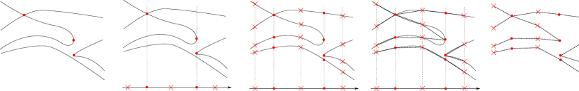
Figure 3.1: The figure on the left shows a curve $C$ with two $x$-extremal points and one singular point (red dots). In the projection phase, these points are projected onto the $x$-axis and rational points separating the $x$-critical values are inserted (red crosses). In the lifting phase, the fibers at the critical values (red dots) and at the points in between (red crosses) are computed. In the connection phase, each pair of points connected by an arc of $C$ is determined, and a corresponding line segment is inserted. Finally, we obtain a graph that is isotopic to $C$.

3.1 Project

We follow a similar approach as in BiProject, that is, we compute the resultant $R(x):=\operatorname{res}(f,f_{y};y)\in\mathbb{Z}[x]$ and a square-free factorization of $R$. In other words, we first determine square-free and pairwise coprime factors $r_{i}\in\mathbb{Z}[x]$, $i=1,\ldots,\deg(R)$, such that $R(x)=\prod_{i=1}^{\deg(R)}\left(r_{i}(x)\right)^{i}$, and then isolate the real roots $\alpha_{i,j}$, $j=1,\ldots,\ell_{i}$, of the polynomials $r_{i}$ which in turn are $i$-fold roots of $R$. The so-obtained isolating intervals have rational endpoints, and we denote $I(\alpha_{i,j})\subset\mathbb{R}$ the interval which contains $\alpha_{i,j}$ but no other root of $r_{i}$. Similar as in Bisolve, we further refine the intervals $I(\alpha_{i,j})$, $i=1,\ldots,\deg(R)$ and $j=1,\ldots,\ell_{i}$, such that all of them are pairwise disjoint. Then, for each pair $\alpha$ and $\alpha^{\prime}$ of consecutive roots of $R$ defining an open interval $I=(\alpha,\alpha^{\prime})$, we choose a separating rational value $q_{I}$ in between the corresponding isolating intervals.

3.2 Lift

Isolating the roots of the intermediate polynomials $f(q_{I},y)$ is straight-forward because each $f(q_{I},y)$ is a square-free polynomial with rational coefficients, and thus the Descartes method directly applies.

Determining the roots of $f_{\alpha}(y):=f(\alpha,y)\in\mathbb{R}[y]$ at an $x$-critical value $\alpha$ is considerably more complicated because $f_{\alpha}$ has multiple roots and, in general, irrational coefficients. One of the main contributions of this paper is to provide novel methods to compute the fiber at an $x$-critical value $x=\alpha$. More precisely, we first present a complete and certified method Lift-BS which is based on Bisolve (taken from Section 2). It applies to any input curve (without assuming generic position) and any corresponding $x$-critical value; see Section 3.2.1. In Section 3.2.2, we further present a certified symbolic-numeric method denoted Lift-NT. Compared to Lift-BS, it shows better efficiency in practice, but it may fail for a few fibers if the input curve is in a special geometric situation. We further provide a method in order to easily check in advance whether Lift-NT will succeed, and we also prove that this can always be achieved by means of a random coordinate transformation. As already mentioned in the introduction, we aim to avoid such a transformation for efficiency reasons. Hence, we propose to combine both lifting methods in way such that Lift-NT runs by default, and, only in case of its failure, we fall back to Lift-BS.

3.2.1 Lift-BS — a complete method for fiber computation

Lift-BS is based on the algorithm Bisolve to isolate the real solutions of a system of two bivariate polynomials $f,g\in\mathbb{Z}[x,y]$. Recall that Bisolve returns a set of disjoint boxes $B_{1},\ldots,B_{m}\subset\mathbb{R}^{2}$ such that each box $B_{i}$ contains exactly one real solution $\xi=(x_{0},y_{0})$ of $f(x,y)=g(x,y)=0$, and the union of all $B_{i}$ covers all solutions. Furthermore, for each solution $\xi$, Bisolve provides square-free polynomials $p,q\in\mathbb{Z}[x]$ with $p(x_{0})=q(y_{0})=0$ and corresponding isolating (and refineable) intervals $I(x_{0})$ and $I(y_{0})$ for $x_{0}$ and $y_{0}$, respectively. Comparing $\xi$ with another point $\tilde{\xi}=(x_{1},y_{1})\in\mathbb{R}^{2}$ given by a similar representation is rather straight-forward. Namely, let $\tilde{p},\tilde{q}\in\mathbb{Z}[x]$ be corresponding defining square-free polynomials and $I(x_{1})$ and $I(y_{1})$ isolating intervals for $x_{1}$ and $y_{1}$, respectively, then we can compare the $x$- and $y$-coordinates of the points $\xi$ and $\tilde{\xi}$ via $\gcd$-computation of the defining univariate polynomials and sign evaluation at the endpoints of the isolating intervals (see (24, Algorithm 10.44) for more details).

In order to compute the fiber at a specific real $x$-critical value $\alpha$ of $C$, we proceed as follows: We first use Bisolve to determine all solutions $p_{i}=(\alpha,\beta_{i})$, $i=1,\ldots,l$, of the system $f=f_{y}=0$ with $x$-coordinate $\alpha$. Then, for each $p_{i}$, we compute

$$k_{i}:=\min\{k:f_{y^{k}}(\alpha,\beta_{i})=\frac{\partial^{k}f}{\partial y^{k}}(\alpha,\beta_{i})\neq 0\}\geq 2.$$

The latter computation is done by iteratively calling Bisolve for $f_{y}=f_{y^{2}}=0$, $f_{y^{2}}=f_{y^{3}}=0$, and so on, and, finally, by restricting and sorting the solutions along the vertical line $x=\alpha$. We eventually obtain disjoint intervals $I_{1},\ldots,I_{l}$ and corresponding multiplicities $k_{1},\ldots,k_{l}$ such that $\beta_{j}$ is a $k_{j}$-fold root of $f_{\alpha}$ which is contained in $I_{j}$. The intervals $I_{j}$ already separate the roots $\beta_{j}$ from any other multiple root of $f_{\alpha}$, however, $I_{j}$ might still contain ordinary roots of $f_{\alpha}$. Hence, we further refine each $I_{j}$ until we can guarantee via interval arithmetic that $\frac{\partial^{k_{j}}f}{\partial y^{k_{j}}}(\alpha,y)$ does not vanish on $I_{j}$. If the latter condition is fulfilled, then $I_{j}$ cannot contain any root of $f_{\alpha}$ except $\beta_{j}$ due to the Mean Value Theorem. Thus, after refining $I_{j}$, we can guarantee that $I_{j}$ is isolating. It remains to isolate the ordinary roots of $f_{\alpha}$:

We consider the so-called Bitstream Descartes isolator (35) (Bdc for short) which constitutes a variant of the Descartes method working on polynomials with interval coefficients. This method can be used to get arbitrary good approximations of the real roots of a polynomial with “bitstream” coefficients, that is, coefficients that can be approximated to arbitrary precision. Bdc starts from an interval guaranteed to contain all real roots of a polynomial and proceeds with interval subdivisions giving rise to a subdivision tree. Accordingly, the approximation precision for the coefficients is increased in each step of the algorithm. Each leaf of the tree is associated with an interval $I$ and stores a lower bound $l(I)$ and an upper bound $u(I)$ for the number of real roots of $f_{\alpha}$ within this interval based on Descartes’ Rule of Signs. Hence, $u(I)=0$ implies that $I$ contains no root and thus can be discarded. If $l(I)=u(I)=1$, then $I$ is an isolating interval for a simple root. Intervals with $u(I)>1$ are further subdivided. We remark that, after a number of iterations, Bdc isolates all simple roots of a bitstream polynomial, and intervals not containing any root are eventually discarded. For a multiple root $\xi$, Bdc determines an interval $I$ which approximates $\xi$ to an arbitrary good precision but never certifies such an interval $I$ to be isolating.

Now, in order to isolate the ordinary roots of $f_{\alpha}$, we modify Bdc in the following way: We discard an interval $I$ if one of following three cases applies: i) $u(I)=0$, or ii) $I$is completely contained in one of the intervals $I_{j}$, or iii) $I$contains an interval $I_{j}$ and $u(I)\leq k_{j}$. Namely, in each of these situations, $I$ cannot contain an ordinary root of $f_{\alpha}$. An interval $I$ is stored as isolating for an ordinary root of $f_{\alpha}$ if $l(I)=u(I)=1$, and $I$ intersects no interval $I_{j}$. All intervals which do not fulfill one of the above conditions are further subdivided. In a last step, we sort the intervals $I_{j}$ (isolating the multiple roots) and the newly obtained isolating intervals for the ordinary roots along the vertical line.

We remark that, in our implementation, Bisolve applied in Lift-BS reuses the resultant $\operatorname{res}(f,f_{y};y)$ which has already been computed in the projection phase of the algorithm. Furthermore, it is a local approach in the sense that its cost is almost proportional to the number of $x$-critical fibers that have to be considered. This will turn out to be beneficial in the overall approach, where most fibers can successfully be treated by Lift-NT; see Section 3.2.3.

3.2.2 Lift-NT— a symbolic-numeric approach for fiber computation

Many of the existing algorithms to isolate the roots of $f_{\alpha}(y)=f(\alpha,y)$ are based on the computation of additional (combinatorial) information about $f_{\alpha}$ such as the degree $k=k_{\alpha}$ of $\gcd(f_{\alpha},f_{\alpha}^{\prime})$, or the number $m=m_{\alpha}$ of distinct real roots of $f_{\alpha}$; for instance, in (13), the values $m$ and $k$ are determined by means of computing a subresultant sequence before using a variant of the Bdc method (denoted $m$-$k$-Descartes) to eventually isolate the roots of $f_{\alpha}$. Unfortunately, the additional symbolic operations for computing the entire subresultant sequence have turned out to be very costly in practice. The following consideration will show that the number $n_{\alpha}$ ($=\deg(f_{\alpha})-k_{\alpha}$) of distinct complex roots of $f_{\alpha}$ can be computed by means of resultant and gcd computations, and a single modular subresultant computation only. In order to do so, we first compute an upper bound $n_{\alpha}^{+}$ for each $n_{\alpha}$, where $n_{\alpha}^{+}$ has the following property:

$$\text{If }C\text{ has no vertical asymptote at }x=\alpha,\text{ and each critical point }(\alpha,\beta)\text{ (i.e.~{}}f_{x}(\alpha,\beta)$$

$$=f_{y}(\alpha,\beta)=0\text{) on the vertical line }x=\alpha\text{ is also located on }C\text{, then }n_{\alpha}=n_{\alpha}^{+}.$$ (3.1)

We will later see that the condition in (3.1) is always fulfilled if $C$ is in a generic location. From our experiments, we report that, for almost all considered instances, the condition is fulfilled for all fibers. Only for a very few instances, we observed that $n_{\alpha}\neq n_{\alpha}^{+}$ for a small number of fibers. In order to check in advance whether $n_{\alpha}=n_{\alpha}^{+}$ for all $x$-critical values $\alpha$, we will later introduce an additional test that uses a single modular computation and a semi-continuity argument.

Computation of $\mathbf{n_{\alpha}^{+}}$

The following result due to Teissier (17, 18) is crucial for our approach:

Lemma 2 (Teissier).

For an $x$-critical point $p=(\alpha,\beta)$ of $C$, it holds that

$$\operatorname{mult}(f(\alpha,y),\beta)=\operatorname{Int}(f,f_{y},p)-\operatorname{Int}(f_{x},f_{y},p)+1,$$ (3.2)

where $\operatorname{mult}(f(\alpha,y),\beta)$ denotes the multiplicity of $\beta$ as a root of $f(\alpha,y)\in\mathbb{R}[y]$, $\operatorname{Int}(f,f_{y},p)$ the intersection multiplicity of the curves implicitly defined by $f=0$ and $f_{y}=0$ at $p$, and $\operatorname{Int}(f_{x},f_{y},p)$ the intersection multiplicity of $f_{x}=0$ and $f_{y}=0$ at $p$.

Remark 1.

In the case, where $f_{x}$ and $f_{y}$ share a common non-trivial factor $h=\gcd(f_{x},f_{y})\in\mathbb{Z}[x,y]\backslash\mathbb{Z}$, $h$ does not vanish on any $x$-critical point $p$ of $C$, that is, the curves $h=0$ and $f=0$ only intersect at infinity. Namely, $h(p)=0$ for some $p\in\mathbb{C}^{2}$ would imply that $\operatorname{Int}(f_{x},f_{y},p)=\infty$ and, thus, $\operatorname{Int}(f,f_{y},p)=\infty$ as well, a contradiction to our assumption on $f$ to be square-free. Hence, we have $\operatorname{Int}(f_{x},f_{y},p)=\operatorname{Int}(f_{x}^{*},f_{y}^{*},p)$ with $f_{x}^{*}:=f_{x}/h$ and $f_{y}^{*}:=f_{y}/h$. Hence, the following more general formula (which is equivalent to (3.2) for trivial $h$) applies:

$$\operatorname{mult}(f(\alpha,y),\beta)=\operatorname{Int}(f,f_{y},p)-\operatorname{Int}(f_{x}^{*},f_{y}^{*},p)+1.$$ (3.3)

We now turn to the computation of the upper bound $n_{\alpha}^{+}$. We distinguish the cases $\deg f_{\alpha}\neq\deg_{y}f$ and $\deg f_{\alpha}=\deg_{y}f$. In the first case, where $C$ has a vertical asymptote at $\alpha$, we define $n_{\alpha}^{+}:=\deg f_{\alpha}$ which is obviously an upper bound for $n_{\alpha}$. In the case $\deg f_{\alpha}=\deg_{y}f$, the formula (3.3) yields:

$$n_{\alpha} =\#\{\text{distinct complex roots of }f_{\alpha}\}=\deg_{y}f-\deg\gcd(f(\alpha,y),f_{y}(\alpha,y))$$

$$=\deg_{y}f-\sum_{\begin{subarray}{c}\beta\in\mathbb{C}:\\ \makebox[14.00003pt][c]{\scriptsize$f(\alpha,\beta)=0$}\end{subarray}}(\operatorname{mult}(f(\alpha,y),\beta)-1)$$

$$=\deg_{y}f-\sum_{\begin{subarray}{c}\beta\in\mathbb{C}:\\ \makebox[14.00003pt][c]{\scriptsize$(\alpha,\beta)$ is $x$-critical}\end{subarray}}\left(\operatorname{Int}(f,f_{y},(\alpha,\beta))-\operatorname{Int}(f_{x}^{*},f_{y}^{*},(\alpha,\beta))\right)$$

$$=\deg_{y}f-\operatorname{mult}(R,\alpha)+\sum_{\begin{subarray}{c}\beta\in\mathbb{C}:\\ \makebox[17.50003pt][c]{\scriptsize$(\alpha,\beta)$ is $x$-critical}\end{subarray}}\operatorname{Int}(f_{x}^{*},f_{y}^{*},(\alpha,\beta))$$ (3.4)

$$\leq\deg_{y}f-\operatorname{mult}(R,\alpha)+\sum_{\beta\in\mathbb{C}}\operatorname{Int}(f_{x}^{*},f_{y}^{*},(\alpha,\beta))$$ (3.5)

$$=\deg_{y}f-\operatorname{mult}(R,\alpha)+\operatorname{mult}(Q,\alpha)=:n_{\alpha}^{+}$$ (3.6)

where $R(x)=\operatorname{res}(f,f_{y};y)$ and $Q(x):=\operatorname{res}(f_{x}^{*},f_{y}^{*};y)$. The equality (3.4) is due to the fact that $f$ has no vertical asymptote at $\alpha$ and, thus, the multiplicity $\operatorname{mult}(R,\alpha)$ equals the sum $\sum_{\beta\in\mathbb{C}}\operatorname{Int}((f,f_{y},(\alpha,\beta))$ of the intersection multiplicities of $f$ and $f_{y}$ in the fiber at $\alpha$. (3.6) follows by an analogous argument for the intersection multiplicities of $f_{x}^{*}$ and $f_{y}^{*}$ along the vertical line at $\alpha$. From the square-free factorization of $R$, the value $\operatorname{mult}(R,\alpha)$ is already computed, and $\operatorname{mult}(Q,\alpha)$ can be determined, for instance, by computing $Q$, its square-free factorization and checking whether $\alpha$ is a root of one of the factors. The following theorem shows that, if the curve $C$ is in generic position, then $C$ has no vertical asymptote or a vertical line, and $f_{x}^{*}$ and $f_{y}^{*}$ do not intersect at any point above $\alpha$ which is not located on $C$. In the latter case, the inequality (3.5) becomes an equality, and thus $n_{\alpha}=n^{+}_{\alpha}$.

Theorem 5.

For a generic $s\in\mathbb{R}$ (i.e. for all but finitely many), the sheared curve

$$C_{s}:=\{(x,y)\in\mathbb{R}^{2}:f(x+s\cdot y,y)=0\}$$

yields $n_{\alpha}^{+}=n_{\alpha}$ for all $x$-critical values $\alpha$ of $C_{s}$.

Proof.

For a generic $s$, the leading coefficient of $f(x+sy,y)$ (considered as a polynomial in $y$) is a constant, hence we can assume that $C$ has no vertical asymptote and contains no vertical line. We can further assume that $f_{x}$ and $f_{y}$ do not share a common non-trivial factor $h$. Otherwise, we have to remove $h$ first; see also Remark 1. Let $g(x,y)=f(x+sy,y)\in\mathbb{R}[x,y]$ denote the defining equation of the sheared curve $C_{s}$, then the critical points of $C_{s}$ are the common solutions of

$$g_{x}(x,y)=f_{x}(x+sy,y)=0\quad\text{and}\quad g_{y}(x,y)=f_{x}(x+sy)\cdot s+f_{y}(x+sy,y)=0.$$

Hence, the critical points of $C_{s}$ are exactly the points $(\alpha^{\prime},\beta^{\prime})=(\alpha-s\beta,\beta)$, where $(\alpha,\beta)$ is a critical point of $C$. We now consider a specific $(\alpha,\beta)$ and show that, for a generic $s$, the polynomial $g(\alpha^{\prime},y)$ has either no multiple root or exactly one multiple root at $y=\beta^{\prime}=\beta$, where $(\alpha^{\prime},\beta^{\prime})=(\alpha-s\beta,\beta)$ denotes the corresponding critical point of $C_{s}$. Then, the same holds for all critical values $(\alpha^{\prime},\beta^{\prime})$ in parallel because there are only finitely many critical $(\alpha,\beta)$ for $C$. Hence, from the definition of $n_{\alpha^{\prime}}^{+}$, it then follows that $n_{\alpha^{\prime}}^{+}=n_{\alpha^{\prime}}$ for all $x$-critical values $\alpha^{\prime}$ of $C_{s}$. W.l.o.g., we can assume that $(\alpha,\beta)=(0,0)$, and thus $(\alpha^{\prime},\beta^{\prime})=(0,0)$ for the corresponding critical point of $C_{s}$. Let $y^{m}$ be the highest power of $y$ that divides $g(0,y)=f(sy,y)$, and define $f^{*}(s,y):=f(sy,y)/y^{m}$. If there exists an $s_{0}\in\mathbb{R}$ such that $f^{*}(s_{0},y)$ has no multiple root, then we are done. Otherwise, for each $s$, $f^{*}(s,y)$ has a multiple root $y_{0}$ that is different from $0$. It follows that $f^{*}(s,y)$ is not square-free, that is, there exist polynomials $p_{1},p_{2}\in\mathbb{C}[s,y]$ with

$$f^{*}(s,y)=\frac{f(sy,y)}{y^{m}}=p_{1}^{2}(s,y)\cdot p_{2}(s,y)$$ (3.7)

We remark that, for each $s\in\mathbb{C}$, there exists a $y_{s}\in\mathbb{C}\backslash\{0\}$ such that $p_{1}(s,y_{s})=0$. Hence, for $x_{s}:=s/y_{s}$, we have $p_{1}(x_{s}/y_{s},y_{s})=0$, and thus $p_{1}(x/y,y)$ cannot be a power of $y$. Now plugging $s=x/y$, with $y\neq 0$, into (3.7) yields

$$f(x,y)=y^{m}\cdot p_{1}^{2}(x/y,y)\cdot p_{2}(x/y,y)=y^{m}\cdot\left(\frac{\tilde{p}_{1}(x,y)}{y^{m_{1}}}\right)^{2}\cdot\frac{\tilde{p}_{2}(x,y)}{y^{m_{2}}}=y^{m-2m_{1}-m_{2}}\cdot\tilde{p}_{1}^{2}(x,y)\cdot\tilde{p}_{2}(x,y),$$

where $\tilde{p}_{1},\tilde{p}_{2}\in\mathbb{C}[x,y]$, and $m_{1},m_{2}\in\mathbb{N}$. Since $f(x,y)$ is square-free, this is only possible if $\tilde{p}_{1}(x,y)$ is a power of $y$. This implies that $p_{1}(x/y,y)=\tilde{p}_{1}(x,y)/y^{m_{1}}$ is also a power of $y$, a contradiction. ∎

We remark that, in the context of computing the topology of a planar algebraic curve, Teissier’s formula has already been used in (12, 16). There, the authors apply (3.2) in its simplified form (i.e. $\operatorname{Int}(f_{x},f_{y},p)=0$) to compute $\operatorname*{mult}(\beta,f(\alpha,y))$ for a non-singular point $p=(\alpha,\beta)$. In contrast, we use the formula in its general form and sum up the information along the entire fiber which eventually leads to the upper bound $n_{\alpha}^{+}$ on the number of distinct complex roots of $f_{\alpha}$.

In the next step, we provide a method to check in advance whether the curve $C$ is in a generic position in the sense of Theorem 5. Unfortunately, we see no cheap way to check generic position with respect to a specific $x$-critical fiber $x=\alpha$, that is, whether $n_{\alpha}^{+}$ matches $n_{\alpha}$ for a specific $\alpha$. However, we can derive a global test to decide whether the upper bound $n^{+}_{\alpha}$ matches $n_{\alpha}$ for all fibers. While the evaluation of the corresponding test with exact integer arithmetic is expensive, we can use the same argument to derive a conservative modular test which returns the same answer with very high probability. The test relies on the comparison of an upper bound $N^{+}$ for $\sum_{\alpha}n^{+}_{\alpha}$ (i.e. $N^{+}\geq\sum_{\alpha}n^{+}_{\alpha}\geq N:=\sum_{\alpha}n_{\alpha}$) and a lower bound $N^{-}$ for $N$ (i.e. $N^{-}\leq N=\sum_{\alpha}n_{\alpha}$), where we sum over all (complex) $x$-critical values $\alpha$. Then, $N^{-}=N^{+}$ implies that $n_{\alpha}=n_{\alpha}^{+}$ for all $\alpha$. We now turn to the computation of $N^{-}$ and $N^{+}$. Here, we assume that $f$ has no vertical asymptote and no vertical component (in particular, $\deg_{y}f(\alpha,y)=\deg_{y}f(x,y)=:n_{y}$ for all values $\alpha.$).

Computation of $\mathbf{N^{+}}$

Lemma 3.

The sum over all $n^{+}_{\alpha}$, $\alpha$ a complex $x$-critical value of $C$, yields:

$$(\deg_{x}R^{*}\cdot\deg_{y}f)-\deg_{x}R+\deg_{x}\gcd(R^{\infty},Q),$$

where $Q=\operatorname{res}(f_{x}^{*},f^{*}_{y};y)$, and $\gcd(R^{\infty},Q)$ is defined as the product of all common factors of $R$ and $Q$ with multiplicity according to their occurrence in $Q.$

Proof.

For the first term, note that $\deg_{x}R^{*}$ is the number of distinct complex $x$-critical values for $f$ and, thus, the number of summands in $\sum_{\alpha}n_{\alpha}$. The sum over all multiplicities $\operatorname{mult}(R,\alpha)$ for the roots $\alpha$ of $R$ simply yields the degree of $R.$ Finally, the summation over $\operatorname{mult}(Q,\alpha)$ amounts to removing the factors of $Q$ that do not share a root with $R.$ ∎

We remark that the square-free part $R^{*}$ of the resultant $R$ is already computed in the projection phase of the curve analysis, and thus we already know $\deg_{x}R^{*}$. The additional computation of $Q$ and $\gcd(R^{\infty},Q)$ can be performed over a modular prime field $\mathbb{Z}_{p}$ for some randomly chosen prime $p.$ Then, $\deg_{x}(\gcd(R^{\infty}\bmod p,Q\bmod p))\geq\deg_{x}\gcd(R^{\infty},Q)$, and thus

$$N^{+}:=(\deg_{x}R^{*}\cdot\deg_{y}f)-\deg_{x}R+\deg_{x}(\gcd(R^{\infty}\bmod p,Q\bmod p))$$ (3.8)

constitutes an upper bound for $\sum_{\alpha}n_{\alpha}^{+}$. We remark that the result obtained by the modular computation matches $\sum_{\alpha}n_{\alpha}^{+}$ with very high probability. That is, up to the choice of finitely many “unlucky” primes, we have $N^{+}=\sum_{\alpha}n_{\alpha}^{+}$.

In the next step, we show how to compute a lower bound $N^{-}$ for $N$. In order to understand its construction, we first explain how to exactly compute $N$. We stress that our algorithm never performs this computation.

(Exact) Computation of $\mathbf{N}$

Consider a decomposition of the square-free part $R^{*}$ of the resultant $R=\operatorname{res}(f,f_{y};y)$:

$$R^{*}=R_{1}R_{2}\cdots R_{s},\quad R_{i}\in\mathbb{Z}[x],$$ (3.9)

such that $R_{i}(\alpha)=0$ if and only if $f(\alpha,y)$ has exactly $n_{y}-i$ distinct complex roots. Note that all $R_{i}$ are square-free and pairwise coprime. With $d_{i}:=\deg R_{i}$ the degree of the factor $R_{i}$, it follows that

$$N=\sum_{1\leq i\leq r}(n_{y}-i)\cdot d_{i}.$$

The computation of the decomposition in (3.9) uses subresultants. The $i$-th subresultant polynomial $\operatorname{Sres}_{i}(f,g;y)\allowbreak\in\mathbb{Z}[x,y]$ of two bivariate polynomials $f$ and $g$ with $y$-degrees $m_{y}$ and $n_{y},$ respectively, is defined as the determinant of a Sylvester-like matrix.

$$\operatorname{Sres}_{i}(f,f_{y};y):=\left\lvert\;\begin{matrix}f_{m_{y}}^{(y)}&f_{m_{y}-1}^{(y)}&\cdots&\cdots&f_{2i-n_{y}+2}^{(y)}&y^{n_{y}-i-1}f\\ &\ddots&\ddots&\ddots&\vdots&\vdots\\ &&f_{m_{y}}^{(y)}&\cdots&f_{i+1}^{(y)}&f\\ g_{n_{y}}^{(y)}&g_{n_{y}-1}^{(y)}&\cdots&\cdots&g_{2i-m_{y}+2}^{(y)}&y^{m_{y}-i-1}g\\ &\ddots&\ddots&\ddots&\vdots&\vdots\\ &&g_{n_{y}}^{(y)}&\cdots&g_{i+1}^{(y)}&g\end{matrix}\;\right\rvert\!\!\begin{array}[]{l}\left.\begin{matrix}\vphantom{fg_{m_{y}}^{(y)}}\\ \vphantom{fg_{m_{y}}^{(y)}}\\ \vphantom{fg_{m_{y}}^{(y)}}\end{matrix}\right\}\,\text{\small$n_{y}-i$ rows}\\ \vspace*{-0.95em}\\ \left.\begin{matrix}\vphantom{fg_{m_{y}}^{(y)}}\\ \vphantom{fg_{m_{y}}^{(y)}}\\ \vphantom{fg_{m_{y}}^{(y)}}\end{matrix}\right\}\,\text{\small$m_{y}-i$ rows}\end{array}$$

The subresultants exhibit a direct relation to the number and multiplicities of common roots of $f$ and $g.$ More specifically, it holds that $\deg\gcd(f(\alpha,y),g(\alpha,y))=k$ if and only if the $i$-th principal subresultant coefficient (psc) $\operatorname{sr}_{i}(x):=\operatorname{sres}_{i}(f,g;y):=\operatorname{coeff}_{i}(\operatorname{Sres}_{i}(f,g;y);y)\in\mathbb{Z}[x]$ vanishes at $\alpha$ for all $i=0,\ldots,k-1$, and $\operatorname{sr}_{k}(\alpha)\neq 0$ (e.g. see (36, 37) for a proof).

Thus, the decomposition in (3.9) can be derived as

$$S_{0} :=R^{*}, \qquad S_{i} :=\gcd(S_{i-1},\operatorname{sr}_{i}) \quad\text{ for }i=1,\dots,s,$$ (3.10)

$$R_{1} :=\frac{S_{0}}{\gcd(S_{0},S_{1})}, \qquad R_{i} :=\frac{\gcd(S_{0},\dots,S_{i-1})}{\gcd(S_{0},\dots,S_{i-1},S_{i})} \quad\text{ for }i=1,\dots,s,$$ (3.11)

where $s$ is the number of non-trivial entries in the subresultant sequence of $f$ and $f_{y}.$ The computation of $N$ as described here requires the exact computation of all psc’s, a very costly operation which would affect the overall runtime considerably. Instead, we consider the following modular approach:

Computation of $\mathbf{N^{-}}$

The main idea of our approach is to perform the above subresultant computation over $\mathbb{Z}_{p}$ for a single, randomly chosen prime $p$. More precisely, we denote

$$\operatorname{sr}_{i}^{(p)}(x):=\operatorname{sres}_{i}^{(p)}(f^{(p)},g^{(p)};y):=\operatorname{coeff}_{i}(\operatorname{Sres}_{i}^{(p)}(f^{(p)},g^{(p)};y);y)\in\mathbb{Z}_{p}[x]$$

the $i$-th principle subresultant coefficient in the subresultant sequence of $f^{(p)}:=f\bmod p\in\mathbb{Z}_{p}[x,y]$ and $g^{(p)}:=g\bmod p\in\mathbb{Z}_{p}[x,y]$. The polynomials $S_{i}^{(p)}\in\mathbb{Z}_{p}[x]$ and $R_{i}^{(p)}\in\mathbb{Z}_{p}[x]$ are then defined in completely analogous manner as the polynomials $S_{i}\in\mathbb{Z}[x]$ and $R_{i}\in\mathbb{Z}[x]$ in (3.10) and (3.11), respectively. The following lemma shows that this yields a lower bound for $N$ if $p$ does not divide the leading coefficient of $f$ and $f_{y}$:

Lemma 4.

Let $p$ be a prime that does not divide the leading coefficient of $f$ and $f_{y}$, and let $d_{i}^{(p)}:=\deg R_{i}^{(p)}$ denote the degree of $R_{i}^{(p)}$. Then,

$$N^{-}:=\sum_{i\geq 1}(n_{y}-i)\cdot d_{i}^{(p)}$$ (3.12)

constitutes a lower bound for the total number $N$ of distinct points on $C$ in $x$-critical fibers.

Proof.

It suffices to show that $\sum_{i\geq 1}i\cdot d_{i}\leq\sum_{i\geq 1}i\cdot d_{i}^{(p)}.$ Namely, using $d:=\deg R^{*}=\sum_{i\geq 1}d_{i}=\sum_{i\geq 1}d_{i}^{(p)},$ we obtain

$$N^{-}=\sum_{i\geq 1}(n_{y}-i)\cdot d_{i}^{(p)}=n_{y}d-\sum_{i\geq 1}i\cdot d_{i}^{(p)}\leq n_{y}d-\sum_{i\geq 1}i\cdot d_{i}=\sum_{i\geq 1}(n_{y}-i)\cdot d_{i}=N.$$

Since $p$ does not divide the leading coefficient of $f$ and $f_{y}$, we have $\operatorname{sr}_{i}^{(p)}=\operatorname{sr}_{i}\bmod p$ due to the specialization property of subresultants. Hence, $n_{i}^{(p)}:=\deg S_{i}^{(p)}\geq n_{i}:=\deg S_{i}$ which implies the following diagram (with some $t$ such that $s\leq t\leq n$)

$$\begin{array}[]{r@{\;}*{13}{c@{\;}}l}d=&n_{0}^{(p)}&\geq&n_{1}^{(p)}&\geq&\cdots&\geq&n_{s}^{(p)}&\geq&n_{s+1}^{(p)}&\geq&\cdots&\geq&n_{t}^{(p)}&=0\\[2.15277pt] &\parbox[c]{0.0pt}{\rotatebox{-90.0}{$=$}}&&\parbox[c]{0.0pt}{\rotatebox{-90.0}{$\geq$}}&&&&\parbox[c]{0.0pt}{\rotatebox{-90.0}{$\geq$}}&&\parbox[c]{0.0pt}{\rotatebox{-90.0}{$\geq$}}&&&&\parbox[c]{0.0pt}{\rotatebox{-90.0}{$=$}}\\[2.15277pt] d=&n_{0}&\geq&n_{1}&\geq&\cdots&\geq&n_{s}&=&n_{s+1}&=&\cdots&=&n_{t}&=0\end{array}$$

Furthermore, we have $d_{i}=n_{i-1}-n_{i}$ and $d_{i}^{(p)}=n_{i-1}^{(p)}-n_{i}^{(p)}.$ Thus,

$$\sum_{i\geq 1}i\cdot d_{i}=\sum_{i\geq 1}\sum_{j\geq i}^{s}d_{j}=\sum_{i\geq 1}\sum_{j\geq i}^{s}(n_{j-1}-n_{j})=\sum_{i\geq 1}n_{i-1}=\sum_{i\geq 0}n_{i}\quad(\text{since }n_{i}=0\text{ for }i\geq s)$$

and, analogously, $\sum_{i\geq 1}i\cdot d_{i}^{(p)}=\sum_{i\geq 0}n_{i}^{(p)}.$ This shows $\sum_{i\geq 1}i\cdot d_{i}\leq\sum_{i\geq 1}i\cdot d_{i}^{(p)}$. ∎

We remark that, for all but finitely many (unlucky) choices of $p,$ all polynomials $R_{i}$ and $R^{(p)}_{i}$ have the same degree. Thus, with high probability, $N^{-}$ as defined in (3.12) matches $N$. In addition, also with very high probability, we have $N^{+}=\sum_{\alpha}n^{+}_{\alpha}$. Hence, if the curve $C$ is in generic position and our choice of $p$ is not unlucky, then $N^{-}=N^{+}=N$, and thus we can certify in advance that $n_{\alpha}=n_{\alpha}^{+}$ for all $x$-critical values $\alpha$. We would like to emphasize that the only exact computation (over $\mathbb{Z}$) that is needed for this test is that of the square-free part of the resultant $R$ (more precisely, only that of its degree). All other operations can be performed over $\mathbb{Z}_{p}$ for a single, randomly chosen prime $p$. Putting everything together now yields our method Lift-NT to compute the fiber at an $x$-critical value:

Lift-NT

We consider a hybrid method to isolate all complex roots and, thus, also the real roots of $f_{\alpha}(y)=f(\alpha,y)\in\mathbb{R}[y]$, where $\alpha$ is a real valued $x$-critical value of the curve $C$. It combines (a) a numerical solver to compute arbitrary good approximations (i.e. complex discs in $\mathbb{C}$) of the roots of $f_{\alpha}$, (b) an exact certification step to certify the existence of roots within the computed discs, and (c) additional knowledge on the number $n_{\alpha}$ of distinct (complex) roots of $f_{\alpha}$. Lift-NT starts with computing the upper bound $n_{\alpha}^{+}$ for $n_{\alpha}$ and the values $N^{-}$ and $N^{+}$ as defined in (3.6), (3.12), and (3.8), respectively. We distinguish two cases:

• $N^{-}=N^{+}$: In this case, we know that $n_{\alpha}=n_{\alpha}^{+}$. We now use a numerical solver to determine disjoint discs $D_{1},\ldots,D_{m}\subset\mathbb{C}$ and an exact certification step to certify the existence of a certain number $m_{i}\geq 1$ of roots (counted with multiplicity) of $f_{\alpha}$ within each $D_{i}$; see A for details. Increasing the working precision and the number of iterations within the numerical solver eventually leads to arbitrary well refined discs $D_{i}$ – but without a guarantee that these discs are actually isolating! However, from a certain iteration on, the number of discs certified to contain at least one root matches $n_{\alpha}$. When this happens, we know for sure that the $D_{i}$’s are isolating. We can then further refine these discs until, for all $i=1,\ldots,m$,

  $$D_{i}\cap\mathbb{R}=\emptyset\text{ or }\bar{D}_{i}\cap D_{j}=\emptyset\text{ for all }j\neq i,$$ (3.13)

  where $\bar{D}_{i}:=\{\bar{z}:z\in D_{i}\}$ denotes the complex conjugate of $D_{i}$. The latter condition guarantees that each disc $D_{i}$ which intersects the real axis actually isolates a real root of $f_{\alpha}$. In addition, for each real root isolated by some $D_{i}$, we further obtain its multiplicity $m_{i}$ as a root of $f_{\alpha}$.

• $N^{-}<N^{+}$: In this case, we have either chosen an unlucky prime in some of the modular computations, or the curve $C$ is located in a special geometric situation; see (3.1) and Theorem 5. However, despite the fact that there might exist a few critical fibers where $n_{\alpha}<n_{\alpha}^{+}$, there is still a good chance that equality holds for most $\alpha$. Hence, we propose to use the numerical solver as a filter in a similar manner as in the case, where $N^{-}=N^{+}$. More precisely, we run the numerical solver on $f_{\alpha}$ for a certain number of iterations. Since $n_{\alpha}^{+}$ constitutes an upper bound on the number of distinct complex roots of $f_{\alpha}$, we must have $m\leq n_{\alpha}\leq n_{\alpha}^{+}$ at any time. Hence, if the number $m$ equals $n_{\alpha}^{+}$, we know for sure that all complex roots of $f_{\alpha}$ are isolated and can then proceed as above. If, after a number of iterations, it still holds that $m<n_{\alpha}^{+}$, Lift-NT reports a failure.

Lift-NT is a certified method, that is, in case of success, it returns the mathematical correct result. However, in comparison to the complete method Lift-BS, Lift-NT may not apply to all critical fibers if the curve $C$ is in a special geometric situation. We would like to remark that, for computing the topology of the curve $C$ only, we can exclusively use Lift-NT as the lifting method. Namely, when considering, as indicated earlier, an initial shearing $x\mapsto x+s\cdot y$, with $s$ a randomly chosen integer, the sheared curve

$$C_{s}:=\{(x,y)\in\mathbb{R}^{2}:f(x+s\cdot y,y)=0\}$$

is in generic situation (with high probability) due to Theorem 5. Then, up to an unlucky choice of prime numbers in the modular computations, we obtain bounds $N^{-}$ and $N^{+}$ for $N$ which are equal. Hence, up to an unlucky choice of finitely many "bad" shearing parameters $s$ and primes $p$, the curve $C_{s}$ is in a generic situation, and, in addition, we can actually prove this. It follows that $n_{\alpha}^{+}=n_{\alpha}$ for all $x$-critical values of the sheared curve $C_{s}$, and thus Lift-NT is successful for all fibers. Since the sheared curve is isotopic to $C$, this shows that we can always compute the topology of $C$ by exclusively using Lift-NT during the lifting phase.

3.2.3 Lift— Combining Lift-BS and Lift-NT

We have introduced two different methods to compute the fibers at the $x$-critical values of a curve $C$. Lift-BS is certified and complete, but turns out to be less efficient than Lift-NT which, in turn, may fail for a few fibers for curves in a special geometric situation. Hence, in the lifting step, we propose to combine the two methods. That is, we run Lift-NT by default, and fall back to Lift-BS only if Lift-NT fails. In practice, as observed in our experiments presented in Section 6.2, the failure conditions for Lift-NT are almost negligible, that is, the method only fails for a few critical fibers for some curves in a special geometric situation. In addition, in case of a failure, we profit from the fact that our backup method Lift-BS applies very well to a specific fiber. That is, its computational cost is almost proportional to the number of fibers that are considered.

We also remark that, for the modular computations of $N^{-}$ and $N^{+}$, we never observed any failure when choosing a reasonable large prime. However, it should not be concealed that we only performed these computations off-line in Maple. Our C++-implementation still employs a more naive approach, where we always use Lift-NT as a filter as described in the case $N^{-}<N^{+}$ above.

In the last section, we mentioned that Lift-NT can be turned into a complete method when considering an initial coordinate transformation. Hence, one might ask why we do not consider such a transformation to compute the topology of $C$. There are several reasons to not follow this approach. Namely, when considering a shearing, the algorithm computes the topology of $C$, but does not directly yield a geometric-topological analysis of the curve since the vertices of the so-obtained graph are not located on $C$. In order to achieve the latter as well, we still have to "shear back" the information for the sheared curve, an operation which is non-trivial at all; see (13) for details. Even though the latter approach seems manageable for a single curve, it considerably complicates the arrangement computation (see Section 4) because the majority of the input curves can be treated in the initial coordinates. Furthermore, in particular for sparse input, a coordinate transformation induces considerably higher computational costs in all subsequent operations.

3.3 Connect

Let us consider a fixed $x$-critical value $\alpha$, the corresponding isolating interval $I(\alpha)=(a,b)$ computed in the projection phase and the points $p_{i}:=(\alpha,y_{\alpha,i})\in C$, $i=1,\ldots,m_{\alpha}$, located on $C$ above $\alpha$. Furthermore, let $I=(\alpha,\alpha^{\prime})$ be the interval connecting $\alpha$ with the nearest $x$-critical value to the right of $\alpha$ (or $+\infty$ if none exists) and $A_{j}$, $j=1,\ldots,m_{I}$, the $j$-th arc of $C$ above $I$ with respect to vertical ordering. $A_{j}$ is represented by a point $a_{j}:=(q_{I},y_{I,j})\in C$, where $y_{I,j}$ denotes the $j$-th real root of $f(q_{I},y)$ and $q_{I}$ an arbitrary but fixed rational value in $I$. To its left, $A_{j}$ is either connected to $(\alpha,\pm\infty)$ (in case of a vertical asymptote) or to one of the points $p_{i}$. In order to determine the point to which an arc $A_{j}$ is connected, we consider the following two distinct cases:

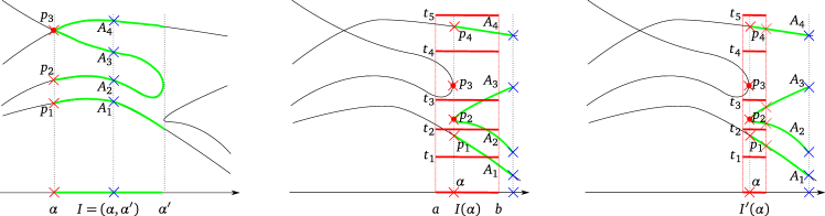
Figure 3.2: The left figure shows the generic case, where exactly one $x$-critical point ($p_{3}$) above $\alpha$ exists. The bottom-up method connects $A_{1}$ to $p_{1}$ and $A_{2}$ to $p_{2}$; the remaining arcs have to pass $p_{3}$. In the second figure, the fiber at $\alpha$ contains two critical points $p_{2}$ and $p_{3}.$ The red horizontal line segments pass through arbitrary chosen points $(\alpha,t_{i})$ separating $p_{i-1}$ and $p_{i}$. The initial isolating interval $I(\alpha)=(a,b)$ for $\alpha$ is not sufficient to determine the connections for all arcs since $A_{1},A_{2},A_{3}$ intersect the segments $I\times\{t_{i}\}.$ On the right, the refined isolating interval $I^{\prime}(\alpha)$ induces boxes $I^{\prime}(\alpha)\times(t_{i},t_{i+1})$ small enough such that no arc crosses the horizontal boundaries. By examination of the $y$-coordinates of the intersections between the arcs and the fiber over the right-hand boundary of $I^{\prime}(\alpha)$ (red crosses), we can match arcs and critical points.

• The generic case, that is, there exists exactly one real $x$-critical point $p_{i_{0}}$ above $\alpha$ and $\deg f(\alpha,y)=\deg_{y}f$. The latter condition implies that $C$ has no vertical asymptote at $\alpha$. Then, the points $p_{1},\ldots,p_{i_{0}-1}$ must be connected with $A_{1},\ldots,A_{i_{0}-1}$ in bottom-up fashion, respectively, since, for each of these points, there exists a single arc of $C$ passing this point. The same argument shows that $p_{i_{0}+1},\ldots,p_{m_{\alpha}}$ must be connected to $A_{m_{I}-m_{\alpha}+i_{0}+1},\ldots,A_{m_{I}}$ in top-down fashion, respectively. Finally, the remaining arcs in between must all be connected to the $x$-critical point $p_{i_{0}}$.

• The non-generic case: We choose arbitrary rational values $t_{1},\ldots,t_{m_{\alpha}+1}$ with $t_{1}<y_{\alpha,1}<t_{2}<\ldots<y_{\alpha,m_{\alpha}}<t_{m_{\alpha}+1}$. Then, the points $\tilde{p}_{i}:=(\alpha,t_{i})$ separate the $p_{i}$’s from each other. Computing such $\tilde{p}_{i}$ is easy since we have isolating intervals with rational endpoints for each of the roots $y_{\alpha,i}$ of $f(\alpha,y)$. In a second step, we use interval arithmetic to obtain intervals $\mathfrak{B}f(I(\alpha)\times t_{i})\subset\mathbb{R}$ with $f(I(\alpha)\times t_{i})\subset\mathfrak{B}f(I(\alpha)\times t_{i})$. As long as there exists an $i$ with $0\in\mathfrak{B}f(I(\alpha)\times t_{i})$, we refine $I(\alpha)$. Since none of the $\tilde{p}_{i}$ is located on $C$, we eventually obtain a sufficiently refined interval $I(\alpha)$ with $0\notin\mathfrak{B}f(I(\alpha)\times t_{i})$ for all $i$. It follows that none of the arcs $A_{j}$ intersects any line segment $I(\alpha)\times t_{i}$. Hence, above $I(\alpha)$, each $A_{j}$ stays within the rectangle bounded by the two segments $I(\alpha)\times t_{i_{0}}$ and $I(\alpha)\times t_{i_{0}+1}$ and is thus connected to $p_{i_{0}}$. In order to determine $i_{0}$, we compute the $j$-th real root $\gamma_{j}$ of $f(b,y)\in\mathbb{Q}[y]$ and the largest $i_{0}$ such that $\gamma_{j}>t_{i_{0}}$. In the special case where $\gamma_{j}<t_{i}$ or $\gamma_{j}>t_{i}$ for all $i$, it follows that $A_{j}$ is connected to $(\alpha,-\infty)$ or $(\alpha,+\infty)$, respectively.

For the arcs located to the left of $\alpha$, we proceed in exactly the same manner. This concludes the connection phase and, thus, the description of our algorithm.

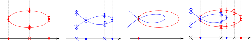
Figure 3.3: The two figures on the left show the topology analyses for the curves $C=V(f)$ and $D=V(g)$. The second figure from the right shows the intersection of the two curves. For the curve pair analysis, critical event lines (at dots) are sorted and non-critical event lines (at crosses) in between are inserted. Finally, for each event line $x=\alpha$, the roots of $f(\alpha,y)$ and $g(\alpha,y)$ are sorted. The latter task is done by further refining corresponding isolating intervals (blue or red intervals) and using the combinatorial information from the curve analyses and the computation of the intersection points.

4 Arrangement computation

Cgal’s prevailing implementation for computing arrangements of planar algebraic curves reduces all required geometric constructions (as intersections) and predicates (as comparisons of points and $x$-monotone curves) to the geometric-topological analysis of a single curve (13) and pairs of curves (1); see also (38) and Cgal’s documentation (2).

In Section 3, we have already seen how to improve the curve-analysis. In a similar way, we want to increase the performance of the analyses of a pair of curves $C=V(f)$ and $D=V(g)$, (see illustration in Figure 3.3). In general, the algorithm from (1) had to compute the entire subresultant sequence, an operation that we are aiming to avoid. Using the new analyses of each single curve and combining the so-obtained information with the information on the intersection points of the two curves $C$ and $D$ as returned by Bisolve, it is straight-forward to achieve this goal. We mainly have to compute the common intersection points of the two curves:

Let $C=V(f)$ and $D=V(g)$ be two planar algebraic curves implicitly defined by square-free polynomials $f$, $g\in\mathbb{Z}[x,y]$. The curve analysis for $C$ provides a set of $x$-critical event lines $x=\alpha$. Each $\alpha$ is represented as the root of a square-free polynomial $r_{i}$, with $r_{i}$ a factor of $R_{C}:=\operatorname{res}(f,f_{y};y)$, together with an isolating interval $I(\alpha)$. In addition, we have isolating intervals for the roots of $f(\alpha,y)$. A corresponding result also holds for the curve $D$ with $R_{D}:=\operatorname{res}(g,g_{y};y)$. For the common intersection points of $C$ and $D$, a similar representation is known. That is, we have critical event lines $x=\alpha^{\prime}$, where $\alpha^{\prime}$ is a root of a square-free factor of $R_{CD}:=\operatorname{res}(f,g;y)$ and, thus, $f(\alpha,y)$ and $g(\alpha,y)$ share at least one common root (or the their leading coefficients both vanish for $x=\alpha$). In addition, isolating intervals for each of these roots have been computed. The curve-pair analysis now essentially follows from merging this information. More precisely, we first compute merged critical event lines (via sorting the roots of $R_{C}$, $R_{D}$ and $R_{CD}$) and, then, insert merged non-critical event lines at rational values $q_{I}$ in between. The intersections of $C$ and $D$ with a non-critical event line at $x=q_{I}$ are easily computed via isolating the roots of $f(q_{I},y)$ and $g(q_{I},y)$ and further refining the isolating intervals until all isolating intervals are pairwise disjoint. For a critical event line $x=\alpha$, we refine the already computed isolating intervals for $f(\alpha,y)$ and $g(\alpha,y)$ until the number of pairs of overlapping intervals matches the number $m$ of intersection points of $C$ and $D$ above $\alpha$. This number is obtained from the output of Bisolve applied to $f$ and $g$, restricted to $x=\alpha$. The information on how to connect the lifted points is provided by the curve analyses for $C$ and $D$. Note that efficiency is achieved by the fact that Bisolve constitute (in its expensive parts) a local algorithm.

We remark that, in the previous approach by Eigenwillig and Kerber (1), $m$ is also determined via efficient filter methods, while, in general, a subresultant computation is needed if the filters fail. This is, for instance, the case when two covertical intersections of $C$ and $D$ occur. For our proposed lifting algorithms, such situations are not more difficult, and thus do not particularly influence the runtime.

5 Speedups

5.1 GPU-accelerated symbolic computations

As mentioned in the introduction, one of the notable advantages of all our new algorithms over similar approaches is that it is not based on sophisticated symbolic computations (such as, for example, evaluating signed remainder sequences) restricting the latter ones to only computing bivariate resultants and gcds of univariate polynomials. In turn, these operations can be outsourced to the graphics hardware to dramatically reduce the overhead of symbolic arithmetic. In this section, we overview the proposed GPU algorithms and refer to (10, 9, 11) for further details.

At the highest level, the resultant and gcd algorithms are based on a modular or homomorphism approach, first exploited in the works of Brown (39) and Collins (40). The modular approach is a traditional way to avoid computational problems, such as expression swell, shared by all symbolic algorithms. In addition, it enables us to distribute the computation of one symbolic expression over a large number of processor cores of the graphics card. Our choice of the target realization platform is not surprising because, with the released CUDA framework (41), the GPU has become a new standard for high-performance scientific computing.

To understand the main principles of GPU computing, we first need to have a look at the GPU architecture. Observe that the parallelism on the graphics processor is supported on two levels. At the upper level, there are numerous thread blocks executing concurrently without any synchronization between them. There is a potentially unlimited number of thread blocks that can be scheduled for execution on the GPU. These blocks are then processed in a queued fashion by the hardware. This realizes block-level parallelism. For its part, each thread block contains a limited number of parallel threads (up to $1024$ threads on the latest GPUs) which can cooperate using on-chip shared memory and synchronize the execution with barriers. This is referred to as thread-level parallelism. An important point is that individual threads running on the GPU are “lite-weight” in a sense that they do not possess large private memory spaces, neither they can execute disjoint code paths without penalties. The conclusion is that an algorithm to be realized on the graphics card must exhibit a high homogeneity of computations such that individual threads can perform the same operations but on different data elements. We start our overview with the resultant algorithm.

Computing resultants in $\mathbb{Z}[x,y]$

Given two bivariate polynomials $f,g\in\mathbb{Z}[x,y]$, the modular resultant algorithm of Collins can be summarized in the following steps:

1. apply a modular homomorphism to map the coefficients of $f$ and $g$ to a finite field for sufficiently many primes $p$: $\mathbb{Z}[x,y]\to\mathbb{Z}_{p}[x,y]$;

2. for each modular image, choose a set of points $\alpha_{p}^{(i)}\in\mathbb{Z}_{p}$, $i\in I$, and evaluate the polynomials at $x=\alpha_{p}^{(i)}$ (evaluation homomorphism): $\mathbb{Z}_{p}[x,y]\to\mathbb{Z}_{p}[x,y]/(x-\alpha_{p}^{(i)})$;

3. compute a set of univariate resultants in $\mathbb{Z}_{p}[x]$ in parallel: $\operatorname{res}_{y}(f,g)|_{\alpha_{p}^{(i)}}:\mathbb{Z}_{m}[x,y]/(x-\alpha_{p}^{(i)})\to\mathbb{Z}_{p}[x]/(x-\alpha_{p}^{(i)})$;

4. interpolate the resultant polynomial for each prime $p$ in parallel: $\mathbb{Z}_{p}[x]/(x-\alpha_{m}{(i)})\to\mathbb{Z}_{p}[x]$;

5. lift the resultant coefficients by means of Chinese remaindering: $\mathbb{Z}_{p}[x]\to\mathbb{Z}[x]$.

Steps (a)–(d) and partly (e) are outsourced to the graphics processor, thereby minimizing the amount of work on the host machine. In essence, what remains to be done on the CPU, is to convert the resultant coefficients in the mixed-radix representation (computed by the GPU) to the standard form.

Suppose we have applied modular and evaluation homomorphisms to reduce the resultant of $f$ and $g$ to $N$ univariate resultants in $\mathbb{Z}_{p}[x]$ for each of $M$ moduli. Thus, provided that the modular images can be processed independently, we can launch a grid of $N\times M$ thread blocks with each block computing the resultant of one modular image. Next, to compute the univariate resultants, we employ a matrix-based approach instead of the classical PRS (polynomial remainder sequences) used by Collins’ algorithm. One of the advantages of this approach is that, when a problem is expressed in terms of linear algebra, all data dependencies are usually made explicit, thereby enabling thread-level parallelism which is a key factor in achieving high performance.

More precisely, the resultants of the modular images are computed by direct factorization of the Sylvester matrix using the so-called Schur algorithm which exploits the special structure of the matrix. In order to give an idea how this algorithm works, let $\tilde{f},\tilde{g}\in\mathbb{Z}[x]$ be polynomials of degrees $m$ and $n$, respectively. Then, for the associated Sylvester matrix $S\in\mathbb{Z}^{r\times r}$ ($r=m+n$), one can write the following displacement equation (42):

$$S-Z_{r}S(Z_{m}\oplus Z_{n})^{T}=GB^{T}\mbox{,}$$ (5.1)

where $Z_{s}\in\mathbb{Z}^{s\times s}$ is a down-shift matrix zeroed everywhere except for 1’s on the first subdiagonal, $\oplus$ denotes the Kronecker sum, and $G,B\in\mathbb{Z}^{r\times 2}$ are the generator matrices whose entries can be deduced from $S$ by inspection. For illustration, we can write (5.1) in explicit form setting $m=4$ and $n=3$:

$$\footnotesize\underbrace{\left[\begin{array}[]{ccccccc}f_{4}&0&0&g_{3}&0&0&0\\ f_{3}&f_{4}&0&g_{2}&g_{3}&0&0\\ f_{2}&f_{3}&f_{4}&g_{1}&g_{2}&g_{3}&0\\ f_{1}&f_{2}&f_{3}&g_{0}&g_{1}&g_{2}&g_{3}\\ f_{0}&f_{1}&f_{2}&0&g_{0}&g_{1}&g_{2}\\ 0&f_{0}&f_{1}&0&0&g_{0}&g_{1}\\ 0&0&f_{0}&0&0&0&g_{0}\\ \end{array}\right]}_{S}-\underbrace{\left[\begin{array}[]{ccccccc}0&0&0&0&0&0&0\\ 0&f_{4}&0&0&g_{3}&0&0\\ 0&f_{3}&f_{4}&0&g_{2}&g_{3}&0\\ 0&f_{2}&f_{3}&0&g_{1}&g_{2}&g_{3}\\ 0&f_{1}&f_{2}&0&g_{0}&g_{1}&g_{2}\\ 0&f_{0}&f_{1}&0&0&g_{0}&g_{1}\\ 0&0&f_{0}&0&0&0&g_{0}\\ \end{array}\right]}_{Z_{r}S(Z_{m}\oplus Z_{n})^{T}}=\underbrace{\left[\begin{array}[]{ccccccc}f_{4}&0&0&g_{3}&0&0&0\\ f_{3}&0&0&g_{2}&0&0&0\\ f_{2}&0&0&g_{1}&0&0&0\\ f_{1}&0&0&g_{0}&0&0&0\\ f_{0}&0&0&0&0&0&0\\ 0&0&0&0&0&0&0\\ 0&0&0&0&0&0&0\\ \end{array}\right]}_{GB^{T}}.$$

The matrix on the right-hand side has rank $2$, and hence it can be decomposed as a product of $r\times 2$ and $2\times r$ matrices $G$ and $B^{T}$. The idea of the Schur algorithm is to rely on this low-rank displacement representation of a matrix to compute its factorization in an asymptotically fast way. Particularly, to factorize the matrix $S$, this algorithm only demands for $\mathcal{O}(r^{2})$ operations in $\mathbb{Z}$; see (42, p. 323). In short, the Schur algorithm is an iterative procedure: In each step, it transforms the matrix generators into a “special form” from which triangular factors can easily be deduced based on the displacement equation (5.1). Using division-free modifications, this procedure can be performed efficiently in a prime field giving rise to the resultant algorithm in $\mathbb{Z}_{p}[x]$; its pseudocode (serial version) can be found in (9, Section 4.2). Now, to port this to the GPU, we assign one thread to one row of each of the generator matrices, that is, to four elements (because $G,B\in\mathbb{Z}^{r\times 2}$). In each iteration of the Schur algorithm, each thread updates its associated generator rows and multiplies them by a $2\times 2$ transformation matrix. Altogether, a univariate resultant can be computed in $\mathcal{O}(r)$ finite field operations using $r$ processors (threads). This explains the basic routine of the resultant algorithm.

The next step of the algorithm, namely polynomial interpolation in $\mathbb{Z}_{p}$, can also be performed efficiently on the graphics card. Here, we exploit the fact that interpolation is equivalent to solving a Vandermonde system, where the Vandermonde matrix has a special structure. Hence, we can again employ the Schur algorithm to solve the system in a small parallel time, see (9, Section 4.3). Finally, in order to obtain a solution in $\mathbb{Z}[x]$, we apply the Mixed-Radix Conversion (MRC) algorithm (43) which reconstructs the integer coefficients of the resultant in the form of mixed-radix (MR) digits. The key feature of this algorithm is that it decouples operations in a finite field $\mathbb{Z}_{p}$ from those in the integer domain. In addition, the computation of MR digits can be arranged in a very structured way allowing for data-level parallelism which can be readily exploited to compute the digits on the GPU.

Computing gcds in $\mathbb{Z}[x]$

The modular gcd algorithm proposed by Brown follows a similar outline as Collins’ algorithm discussed above. For $f,g\in\mathbb{Z}[x]$, it consists of three steps:

1. apply modular homomorphism reducing the coefficients of $f$ and $g$ modulo sufficiently many primes: $\mathbb{Z}[x]\to\mathbb{Z}_{p}[x]$;

2. compute a set of univariate gcds in $\mathbb{Z}_{p}[x]$: $\gcd(f,g)\bmod p:\mathbb{Z}_{p}[x]\to\mathbb{Z}_{p}[x]$;

3. lift the coefficients of a gcd using Chinese remaindering: $\mathbb{Z}_{m}[x]\to\mathbb{Z}[x]$.

Again, we augment the original Brown’s algorithm by replacing the Euclidean scheme (used to compute a gcd of each homomorphic image) with a matrix-based approach. The univariate gcd computation is based on the following theorem.

Theorem 6.

(44) Let $S$ be the Sylvester matrix for polynomials $f,g\in\mathbb{F}[x]$ with coefficients over some field $\mathbb{F}$. If $S$ is put in echelon form, using row transformations only, then the last non-zero row gives the coefficients of $\gcd(f,g)\in\mathbb{F}[x]$.

Suppose $f$ and $g$ have degrees $m$ and $n$, respectively. Theorem 6 asserts that if we triangulate the Sylvester matrix $S\in\mathbb{Z}^{r\times r}$ ($r=n+m$), for instance, by means of Gaussian elimination, we obtain $\gcd(f,g)$ in the last nonzero row of the triangular factor. In order to achieve the latter, we apply the Schur algorithm to the positive-definite matrix $W=S^{T}S$ to obtain the orthogonal (QR) factorization of $S$. In terms of displacements, $W$ can be written as follows (42):

$$W-Z_{r}WZ_{r}^{T}=GJG^{T}\mbox{ with }G\in\mathbb{Z}^{r\times 4},\ J=I_{2}\oplus-I_{2}.$$ (5.2)

Here, $I_{s}$ denotes an $s\times s$ identity matrix. Remark that it is not necessary to compute the entries of $W$ explicitly because the generator matrix $G$ is easily expressible in terms of the coefficients of $f$ and $g$, see (11, Section 2.2). Similarly to the resultants, we can run the Schur algorithm for $W$ in $\mathcal{O}(r)$ time on the GPU using $r$ processors (threads). That is, one thread is assigned to process one row of the generator matrix $G$ ($4$ elements). The source code of a sequential algorithm can be found in (11, Algorithm 1).

From the theoretical perspective, the rest of the GPU algorithm essentially follows the same outline as the one for resultants, with the exception that there is no need for an interpolation step anymore since the polynomials are univariate. Certainly, there is also a number of practical difficulties that need to be clarified. One of them is computing tight upper bounds on the height of a polynomial divisor which is needed to estimate the number of moduli used by the algorithm. The existing theoretical bounds are very pessimistic, and the original algorithm by Brown relies on trial division to reduce the number of homomorphic images. However, this solution is incompatible with parallel processing because the algorithm must be applied incrementally. That is why, in the implementation, we use a number of heuristics to shrink the theoretical worst-case bounds.

Another challenge relates to the fact that it is not always possible to compute the gcd of a modular image by a single thread block (recall that the number of threads per block is limited) while threads from different blocks cannot work cooperatively. Thus, we needed to introduce some “data redundancy” to be able to distribute the computation of a single modular gcd (factorization of the Sylvester matrix) across numerous thread blocks. The details can be found in the paper cited above.

5.2 Filters for Bisolve

Besides the parallel computation of resultants and gcds, the algorithm Bisolve to solve bivariate polynomial systems from Section 2 can be elaborated with a number of filtering techniques to early validate a majority of the candidates:

As first step, we group candidates along the same vertical line (a fiber) at an $x$-coordinate $\alpha$ (a root of $R^{(y)}$) to process them together. This allows us to use extra information on the real roots of $f(\alpha,y)\in\mathbb{R}[y]$ and $g(\alpha,y)\in\mathbb{R}[y]$ for the validation of candidates.

Figure 5.1: (a) Intervals containing the roots of $f(\alpha,y)$ and $g(\alpha,y)$ are refined until they either do not overlap or are fully included in candidate boxes. In the former case, the boxes can be discarded. (b) Unvalidated candidates are passed to bidirectional filter which runs bitstream isolation in another direction

We replace the tests based on interval evaluation (see page 2.3) by a test based on the bitstream Descartes isolator (35) (Bdc) (which has already been used in Lift-BS; see Section 3.2.1). To do so, we apply Bdc to both polynomials $f(\alpha,y)$ and $g(\alpha,y)$ in parallel, which eventually reports intervals that do not share common roots. This property is essential for our filtered version of Validate: a candidate box $B(\alpha,\beta)$ can be rejected as soon as the associated $y$-interval $I(\beta)$ fully overlaps with intervals rejected by Bdc for $f(\alpha,y)$ or $g(\alpha,y)$; see Figure 5.1 (a).

As alternative we could also deploy the numerical solver that is utilized in Lift-NT; see A for details. Namely, it can be modified in way to report active intervals, and thus allows us to discard candidates in non-active intervals. Even more, as the numerical solver reports all (complex) solutions, we can use it as inclusion predicate, too: If we see exactly one overlap of reported discs $\Delta_{f}$ and $\Delta_{g}$ (one for $f(\alpha,y)$, the other for $g(\alpha,y)$, respectively), and this overlap is completely contained in the projection $\Delta(\beta)$ of a candidate polydisc $\Delta(\alpha)\times\Delta(\beta)$, then $(\alpha,\beta)$ must be a solution. Namely, $f(\alpha,y)$ and $g(\alpha,y)$ share at least one common root, and each of these roots must be contained in $\Delta_{f}\cap\Delta_{g}$. By construction, $\Delta(\beta)$ contains at most one root, and thus $\beta$ must be the unique common root of the two polynomials.

Grouping candidates along a fiber $x=\alpha$ also enables us to use combinatorial tests to discard or to certify them. First, when the number of certified solutions reaches $\mathrm{mult}(\alpha)$, the remaining candidates are automatically discarded because each real solution contributes at least once to the multiplicity of $\alpha$ as a root of $R^{(y)}$ (see Theorem 1). Second, if $\alpha$ is not a root of the greatest common divisor $h^{(y)}(x)$ of the leading coefficients of $f$ and $g$, $\mathrm{mult}(\alpha)$ is odd, and all except one candidate along the fiber are discarded, then the remaining candidate must be a real solution. This is because complex roots come in conjugate pairs and, thus, do not change the parity of $\mathrm{mult}(\alpha)$. We remark that, in case where the system (2.1) is in generic position and the multiplicities of all roots of $R$ are odd, the combinatorial test already suffices to certify all solutions without the need to apply the inclusion predicate based on Theorem 4.

Now, suppose that, after the combinatorial test, there are several candidates left within a fiber. For instance, the latter can indicate the presence of covertical solutions. In this case, before using the new inclusion predicate, we can apply the aforementioned filters in horizontal direction as well. More precisely, we construct the lists of unvalidated candidates sharing the same $y$-coordinate $\beta$ and process them along a horizontal fiber. For this step, we initialize the bitstream trees (or the numerical solvers) for $f(x,\beta)\in\mathbb{R}[x]$ and $g(x,\beta)\in\mathbb{R}[y]$ and proceed in exactly the same way as done for vertical fibers; see Figure 5.1 (b). We will refer to this procedure as the bidirectional filter, especially in Section 6.1, where we examine the efficiency of all filters. The (few) candidates that still remain undecided after all filters are applied will be processed by considering the new inclusion predicate.

6 Implementation and experiments

Setup

We have implemented our algorithms in a branch of the bivariate algebraic kernel first released with Cgal version 3.7 in October 2010 (45, 2). Bisolve is a completely new implementation, whereas, for GeoTop and the analyses of pairs, we only replaced the lifting algorithms in Cgal’s original curve- and curve-pair analyses with our new methods based on Lift-NT, Lift-BS and Bisolve. As throughout Cgal, we follow the generic programming paradigm which allows us to choose among various number types for polynomials’ coefficients or intervals’ boundaries and to choose the method used to isolate the real roots of univariate polynomials. For our setup, we rely on the integer and rational number types provided by Gmp 5.0.1 and the highly efficient univariate solver based on the Descartes method contained in Rs (by Fabrice Rouillier (27)), which is also the basis for Isolate in Maple 13 and later versions.

All experiments have been conducted on a 2.8 GHz $8$-Core Intel Xeon W3530 with 8 MB of L2 cache on a Linux platform. For the GPU-part of the algorithm, we have used the GeForce GTX580 graphics card (Fermi Core).

Symbolic Speedups

Our algorithms exclusively rely, as indicated, on two symbolic operations, that is, resultant and $\gcd$ computation. We outsource both computations to the graphics hardware to reduce the overhead of symbolic arithmetic which typically constitutes the main bottleneck in previous approaches. Details about this have been covered in Section 5.1. Beyond that, it is worth noting that our implementation of univariate $\gcd$s on the graphics card is comparable in speed with the one from Ntl running on the host machine. Our explanation for this observation is that, in contrast to bivariate resultants, computing a $\gcd$ of moderate degree univariate polynomials does not provide a sufficient amount of parallelism, and Ntl’s implementation is nearly optimal. Moreover, the time for the initial modular reduction of polynomials, still performed on the CPU, can become noticeably large, thereby neglecting the efficiency of the GPU algorithm. Yet, we find it very promising to perform the modular reduction directly on the GPU which should further speed-up our algorithm.

Contestants

For solving bivariate systems (Section 6.1), we compared Bisolve to the bivariate version of Isolate (based on Rs) and Lgp by Xiao-Shan Gao et al. Both are interfaced using Maple 14. We remark that, for the important substep of isolating the real roots of the elimination polynomial, all three contestants in the ring (including our implementation) use the highly efficient implementation provided by Rs.

When analyzing algebraic curves (Section 6.2) and computing arrangements of algebraic curves (Section 6.3), we compared our new implementation with Cgal’s bivariate algebraic kernel (see (38) and (45)) that has shown excellent performance in exhaustive experiments over existing approaches, namely cad2d and Isotop (14) which is based on Rs. These two other contestants were, except for few example instances, less efficient than Cgal’s implementation, so that we omit further tests with them. Two further reasons can be given: Firstly, we enhanced Cgal’s kernel with GPU-supported resultants and $\gcd$s which makes it more competitive to existing software, but also to GeoTop. Still, slowdowns are observable for singular curves or curves in non-generic position due to its need of subresultants sequences performed on the CPU. For such hard instances, our new algorithms particularly profit from the algorithmic design which avoids costly symbolic operations that can only be performed on the CPU. At this point, we also remark that, even if no GPU is available and all symbolic operations would be carried out solely on the CPU, GeoTop is still much faster for hard instances. Secondly, the contestants based on Rs require as subtask Rs to solve the bivariate polynomial system $f=f_{y}=0$ in the curve-analysis. However, our experiments on bivariate system solving that we report in Section 6.1 show that Bisolve is at least competitive to the current version of Rs and even show in most cases an excellent speed gain over Rs. However, it should not be concealed that Rs is currently getting a very promising polish which uses the computations of a rational univariate representations and modular arithmetic (46). Yacine Bouzidi et al. are about to submit a bivariate kernel based on the updated Rs to Cgal in the spirit of the existing univariate kernel based on Rs; see (47). We are looking forward to compare our analysis and the arrangement computation with this upcoming approach.

All test data sets that we consider in our experiments are available for download.

6.1 Bivariate system solving

(X) special curves (see Table 5 in B for descriptions)
	BS	BS+bstr	BS+bstr+comb	BS+all	BS+all	Isolate	LGP
curve	GPU			GPU	CPU	Maple	Maple
13_sings_9	2.13	1.84	1.48	0.97	1.65	341.93	2.81
FTT_5_4_4	48.03	9.20	9.00	20.51	52.21	256.37	195.65
L4_circles	0.92	1.31	1.62	0.74	1.72	1.31	7.58
L6_circles	3.91	4.23	3.68	2.60	16.16	21.37	51.60
SA_2_4_eps	0.97	0.38	0.32	0.44	4.45	3.31	4.69
SA_4_4_eps	4.77	2.07	1.84	2.01	91.90	158.63	54.51
challenge_12	21.54	5.33	5.44	7.35	18.90	44.02	37.07
challenge_12_1	84.63	12.50	12.50	19.17	72.57	351.62	277.68
compact_surf	12.42	3.45	3.29	4.06	12.18	871.95	12.00
cov_sol_20	28.18	24.05	18.82	5.77	16.57	532.41	171.62
curve24	85.91	87.92	13.93	8.22	25.36	86.04	37.94
curve_issac	2.39	2.72	2.25	0.88	1.82	29.80	3.29
cusps_and_flexes	1.17	1.09	0.86	0.63	1.27	381.51	2.43
degree_7_surf	29.92	13.14	11.92	7.74	90.50	timeout	131.25
dfold_10_6	3.30	2.68	2.73	1.55	17.85	3.35	3.76
grid_deg_10	2.49	2.37	1.30	1.20	2.49	111.20	2.64
huge_cusp	9.64	9.81	6.96	6.44	13.67	timeout	116.67
mignotte_xy	t>600	584.75	252.94	243.16	310.13	564.05	timeout
spider	167.30	77.86	50.61	46.47	216.86	timeout	timeout
swinnerton_dyer	28.39	19.70	18.92	5.28	24.38	71.14	27.92
ten_circles	4.62	4.19	4.13	1.33	3.74	5.77	4.96
(X) pairs of special curves (see Table 5 in B for descriptions)
	BS	BS+bstr	BS+bstr+comb	BS+all	BS+all	Isolate	LGP
pair	GPU			GPU	CPU	Maple	Maple
deg18_7_curves	2.19	2.33	1.74	0.97	2.01	3.50	4.37
hard_one	11.34	10.13	6.46	4.29	82.53	64.50	17.45
large_curves	286.32	260.35	72.50	43.12	35.37	311.61	98.07
spiral29_24	207.47	206.62	30.35	18.57	35.53	215.35	76.50
tryme	64.77	65.55	22.67	18.61	48.21	397.41	107.80
vert_lines	0.60	0.61	0.63	0.47	0.69	5.79	1.20

Table 1: Running times (in seconds, including resultant computations) for solving bivariate system defined by special curves. Bisolve-GPU: our approach with GPU-resultants; Bisolve-CPU: our approach with Cgal’s CPU-resultants; Isolate and Lgp use Maple’s implementation for the resultant computation. Bold face indicates the default setup for Bisolve; timeout: algorithm timed out ($>$ 600 sec)

(R) sets of five random dense curves
	BS	BS+bstr	BS+bstr+comb	BS+all	BS+all	Isolate	LGP
degree, bits	GPU			GPU	CPU	Maple	Maple
6, 0010	0.29	0.33	0.31	0.20	0.38	0.54	0.41
6, 0128	0.47	0.29	0.34	0.26	0.31	0.64	0.66
6, 0512	0.99	0.69	0.56	0.43	0.54	1.76	1.91
6, 2048	5.92	3.18	1.99	1.50	1.85	9.31	9.92
9, 0010	2.06	0.88	0.74	0.36	0.78	1.24	0.88
9, 0128	3.31	1.85	1.04	0.45	0.54	1.50	1.66
9, 0512	7.98	4.81	2.39	0.88	1.07	3.62	4.58
9, 2048	34.12	19.87	11.15	3.75	4.19	19.24	24.66
12, 0010	14.85	4.82	2.46	1.07	2.11	3.96	3.32
12, 0128	20.08	7.90	3.78	1.32	1.59	5.77	6.39
12, 0512	42.73	18.22	10.10	2.45	2.80	19.12	23.17
12, 2048	162.11	68.28	53.03	11.14	11.97	109.67	138.06
15, 0010	56.40	10.64	5.69	1.55	2.66	6.09	5.65
15, 0128	95.35	17.00	10.61	2.01	2.30	8.96	10.46
15, 0512	195.01	41.42	31.16	3.95	4.22	26.06	33.87
15, 2048	timeout	161.00	169.77	19.89	20.45	140.68	190.86
(R) sets of five random sparse curves
	BS	BS+bstr	BS+bstr+comb	BS+all	BS+all	Isolate	LGP
degree, bits	GPU			GPU	CPU	Maple	Maple
6, 0010	0.11	0.10	0.16	0.10	0.13	0.19	0.14
6, 0128	0.28	0.12	0.14	0.11	0.15	0.23	0.21
6, 0512	0.50	0.32	0.24	0.20	0.21	0.48	0.47
6, 2048	3.32	1.28	0.65	0.58	0.68	2.12	2.15
9, 0010	0.20	0.52	0.27	0.18	0.24	0.39	0.31
9, 0128	0.45	0.92	0.33	0.22	0.25	0.51	0.52
9, 0512	1.21	1.82	0.54	0.37	0.40	1.44	1.49
9, 2048	7.52	11.02	1.96	1.21	1.38	7.44	8.42
12, 0010	0.51	0.72	0.55	0.28	0.38	0.65	0.53
12, 0128	1.49	1.61	0.75	0.36	0.36	1.08	1.11
12, 0512	5.17	5.75	1.67	0.66	0.69	3.61	3.83
12, 2048	47.19	42.35	7.98	2.70	2.75	21.25	23.89
15, 0010	3.66	3.33	2.11	1.00	1.39	2.48	2.25
15, 0128	12.14	6.37	3.35	1.25	1.35	4.17	4.27
15, 0512	43.36	19.93	8.52	2.40	2.54	13.95	15.48
15, 2048	408.90	150.49	44.34	10.97	10.98	78.65	89.35

Table 2: Total running times for solving five systems defined by random curves of increasing degree and with increasing bit-lengths. For description of configurations, see Table 1.

Our experiments for this task consist of two parts: In the first part, we consider “special” curves $C=V(f)$, and compute the $x$-critical points of $C$ (i.e. the solutions of $f=f_{y}=0$). The curves are selected in order to challenge different parts of our algorithm (and also other algorithms), and in order to show the efficiency of the considered filtering techniques as given in Section 5.2. For instance, we considered curves with many singularities or high-curvature points which requires many candidates to be tested along each vertical line, or prohibit the use of special filters. Table 1 lists timings for various curves (described in Table 5). In the second part of our experiments, we study the performance of Bisolve on random polynomials with increasing total degrees and coefficient bit-lengths. We refer the reader to Table 2 for the corresponding timings.

In columns $2$–$6$ of Table 1 we see the performance of Bisolve with all filters set off (BS), with bitstream filter enabled only (BS+bstr), with bitstream and combinatorial filter (BS+bstr+comb) and with all filters enabled (BS+all); the latter configuration comes with and without the computation of symbolic operations on the GPU. For the remaining configurations, we only show the timings using the GPU. The corresponding CPU-based timings can easily be obtained by adding the (absolute) difference of the BS+all-columns.

One can observe that our algorithm is, in general, superior to Isolate and Lgp, even if the filters are not used. By comparing columns $2$–$6$ of Table 1, one can see that filtering sometimes results in a significant performance improvement. The combinatorial test is particularly useful when the defining polynomials of the system (2.1) have large degrees and/or large coefficient bit-length while, at the same time, the number of covertical or singular solutions is small compared to the total number of candidates being checked. The bidirectional filter is advantageous when the system has covertical solutions in one direction (say along $y$-axis) which are not cohorizontal. This is essentially the case for cov_sol_20, swinnerton_dyer, ten_circles and curve_issac.

Another strength of our approach relates to the fact that the amount of symbolic operations is crucially reduced. Hence, when the time for computing resultants is dominating, the GPU-based algorithm offers a speed-up by a typical factor of $2$-$5$ (sometimes even more; see, in particular, SA_4_4_eps, degree_7_surf, hard_one) over the version with default resultant implementation. It is also worth mentioning that both Isolate and Lgp benefit from the fast resultant computation available in Maple while Cgal’s default resultant computation is generally much slower than that of Maple.

Table 2 lists timings for experiments with random curves. Each instance consists of five curves of the same degree (dense or sparse) and we report the total time to compute the solutions of five systems of the form $f=f_{y}=0$. In order to analyze the influence of the coefficients’ bit-lengths, we multiplied each curve by $2^{k}$ with $k\in\{128,512,2048\}$ and increased the constant coefficient by one. Since the latter operation constitutes only a small perturbation of the vanishing set of the input system, the number of solutions remains constant while the content of the polynomials’ coefficients also stays trivial. We see that the bidirectional filtering is not of any advantage because the system defined by random polynomials is unlikely to have covertical solutions. However, in this case, most candidates are rejected by the combinatorial check, thereby omitting a (more expensive) test based on Theorem 4. This results in a clear speed-up over a “non-filtered” version. Also, observe that, compared to its contestants, GPU-Bisolve is less vulnerable to increasing the bit-length of coefficients. We have also observed that, for our filtered versions, the time for the validation step is almost independent of the bit-lengths.

Further experiments on solving bivariate systems of interpolated, parameterized, translated or projected curves are listed in C. In all these tests Bisolve outperforms Lgp and Isolate; the CPU-only version of Bisolve is at least as efficient as the contestants, and often even faster. We omit experiments to refine the solution boxes to certain precision as this matches the efficiency of QIR due to the fact that we have algebraic descriptions for the solutions’ $x$- and $y$-coordinates.

6.2 Analysing curves

We next present the experiments comparing the analyses of single algebraic curves for different families of curves: (R) random curves of various degree and bit-lengths of their coefficients, (I) curves interpolated through points on a grid, (S) curves in the two-dimensional parameter space of a sphere, (T) curves that were constructed by multiplying a curve $f(x,y)$ with $f(x,y+1)$, such that each fiber has more than one critical point, (P) projections of intersections of algebraic surfaces in 3D and, finally, (G) sets of three generated curves of same degree: (G.1) bivariate polynomials with random uniform coefficients (non-singular), (G.2) projected intersection curves of a random surface and its $z$-derivative (singular-$f$-$f_{z}$), and (G.3) projected intersection curves of two independently chosen surfaces (singular-$f$-$g$) (X) “special” curves of degrees up to 42 with many singularities or high-curvature points. The random and special curves were already under consideration in Section 6.1 where we only computed their $x$-critical points. All other curves are taken from (15, 4.3). For the curve topology analysis, we consider five different setups:

1. BS+all (i.e. Bisolve with all filters enabled) which is, strictly speaking, not comparable with the curve-analysis as it only computes the solutions of the system $f=f_{y}=0$. Still, it is interesting to see that, for most instances, GeoTop outperforms Bisolve though Bisolve one only solves a subproblem of the curve-analysis.

2. Ak_2 is the bivariate algebraic kernel shipped with Cgal 3.7 but with GPU-supported resultants and $\gcd$s.

3. GeoTop-BS that exclusively uses Lift-BS for the fiber liftings.

4. Top-NT that first applies a random shearing (with a low-bit shearing factor), and, then, exclusively uses Lift-NT for lifting step.

5. GeoTop combines Lift-NT and Lift-BS in the fiber computations as discussed in Section 3.2.3: It uses Lift-NT first, and if it fails for a certain fiber after a certain number of iterations, Lift-BS is considered for this fiber instead.
   We remark that the global modular filter that checks whether Lift-NT is successful for all fibers, is not yet in action. So far, this test has only been implemented within Maple. As expected, it performs very well, that is, the run-times are considerably less than that for the majority of steps in the curve analysis.

GeoTop is our default setting, and its running time also includes the timing for the fiber computations where Lift-NT fails and Lift-BS is applied instead.

(R) sets of five random curves
type, degree, bits	BS+all	Ak_2	GeoTop-BS	Top-NT	GeoTop
dense, 09, 0010	0.36	0.66	1.50	0.29	0.23
dense, 09, 2048	3.75	3.48	10.61	2.03	2.16
dense, 15, 0010	1.55	2.15	5.81	0.96	0.92
dense, 15, 2048	19.89	16.86	54.58	7.74	13.24
sparse, 09, 0010	0.18	1.05	0.54	0.20	0.11
sparse, 09, 2048	1.21	4.46	2.79	1.38	0.68
sparse, 15, 0010	1.00	3.37	3.03	0.71	0.59
sparse, 15, 2048	10.97	22.78	24.85	5.47	5.46
(I) sets of five interpolated curves through points on a grid
degree	BS+all	Ak_2	GeoTop-BS	Top-NT	GeoTop
9	3.70	4.98	9.49	1.59	2.37
12	23.09	27.56	57.91	12.37	13.61
15	214.54	160.36	451.29	69.20	114.63
(S) sets of five parameterized curves on a sphere with 16bit-coefficients
degree	BS+all	Ak_2	GeoTop-BS	Top-NT	GeoTop
6	3.00	12.62	16.12	1.97	1.98
9	30.87	39.74	119.61	27.49	21.37
(T) sets of five curves with a vertically translated copy
degree	BS+all	Ak_2	GeoTop-BS	Top-NT	GeoTop
6	1.32	12.69	8.59	0.77	0.67
9	5.05	134.75	27.93	5.39	2.23
(P) projected intersection curve of surfaces with 8bit-coefficients
degree(s)	BS+all	Ak_2	GeoTop-BS	Top-NT	GeoTop
$6\cdot 6$	1.40	220.02	383.45	2.57	0.68
$8\cdot 8$	21.86	timeout	117.57	19.56	6.17
(G) random singular and non-singular curves
type degree, bits	BS+all	Ak_2	GeoTop-BS	Top-NT	GeoTop
non-singular 42, 237	56.57	40.66	133.12	23.27	35.80
singular-$f$-$f_{z}$ 42, 238	64.24	timeout	372.99	52.27	25.50
singular-$f$-$g$ 42, 237	122.20	timeout	419.16	39.55	18.77
(X) special curves (see Table 5 in B for descriptions)
curve	BS+all	Ak_2	GeoTop-BS	Top-NT	GeoTop
L6_circles	2.60	171.86	108.46	1.61	1.62
SA_4_4_eps	2.01	122.30	11.96	3.92	2.00
challenge_12	7.35	timeout	16.11	64.75	12.50
compact_surf	4.06	81.56	19.66	7.43	5.31
cov_sol_20	5.77	43.40	14.06	4.22	2.41
degree_7_surf	7.74	timeout	57.41	6.23	4.19
dfold_10_6	1.55	35.40	10.74	8.97	0.90
mignotte_xy	243.16	timeout	276.89	199.59	128.05
spider	46.47	timeout	200.61	22.34	21.03
swinnerton_dyer	5.28	347.28	43.78	13.04	6.97
ten_circles	1.33	22.77	11.84	4.26	0.86

Table 3: Running times (in sec) for analyses of algebraic curves of various families; timeout: algorithm timed out ($>$ 600 sec)

Table 3 lists the running times for single-curve analyses. We only give the results for representative examples; full tables are listed in D. From our experiments, we conclude that GeoTop is, in general, superior to the existing kernel, even though Cgal’s original implementation now profits from GPU-accelerated resultants and gcds. Moreover, while the speed-up for curves in generic position is already considerable (about half of the time), it becomes even more impressive for projected intersection curves of surfaces and “special” curves with many singularities. The reason for this tremendous speed-up is that, for singular curves, Ak_2’s performance drops significantly with the degree of the curve when the time to compute subresultants on the CPU becomes dominating. In addition, for curves in non-generic position, the efficiency of Ak_2 is affected because a coordinate transformation has to be considered in these cases.

Recall that Lift-NT in GeoTop fails for very few instances, where Lift-BS is locally used to treat some of the $x$-critical fibers instead. The switch to the backup method is observable in timings; see for instance, challenge_12. Namely, the difference of the running times between GeoTop and GeoTop-BS are considerably less than the difference which can usually be observed for instances where the filter method succeeds for all fibers. In these cases, the numerical solver cannot isolate the roots within a given number of iterations, or we indeed have $n_{\alpha}<n^{+}_{\alpha}$ for some fibers $x=\alpha$; see Section 3.2.2. Nevertheless, the running times are still very promising and yet perform much better than Ak_2 for non-generic input, even though Lift-BS’s implementation is not yet optimized, and we anticipate a further performance improvement.

Similar as Ak_2 has improved on previous approaches when it was presented in 2008, our new methods improve on Ak_2 now. That is, for random, interpolated and parameterized curves, the speed gain is noticeable, while for translated curves and projected intersections, we improve the more the higher the degrees. On some curves of large degree(!), we improve by a factor up to 250 and more.

We also recommend GeoTop over Top-NT since it gives full geometric information at basically no additional cost; that is, for random instances, both are similarly efficient whereas, for non-random input, the winner is often determined by the geometry of the curve. For instance, the projection step in Top-NT is faster than that of GeoTop for random and interpolated curves. We cannot fully explain this observation, but we guess that the initial shearing results in a better separation of the resultant’s roots which makes the real root isolation cheaper. On the other hand, for curves with many covertical critical points (e.g. challenge_12), shearing yields a resultant which decomposes into less but more complex factors, which implies much higher cost to isolate the roots of the resultant polynomial. In addition, we have to consider more $x$-critical fibers, and Lift-NT also has to deal with larger bitlengths. In summary, we propose to not consider a shearing because, from our experiments, we can say that the increased cost are higher than the cost for the few needed runs of Lift-BS, when GeoTop analyses the curve in the original coordinate system. s Unlike existing algorithms, GeoTop exhibits a very robust behavior on singular inputs. In contrast, it often performs even better on singular instances than on non-singular curves which have the same input size. This behavior can be read off in detail from Table 9 in D. where we compare curves of same degree without and with singularities. For large instances, GeoTop noticeably outperforms the other contestants and actually even benefits from singularities. We suspect that this behavior is due to the fact that the resultant splits into many simple factors. Namely, in this case, root isolation of the resultant becomes less costly than in the non-singular case, where the resultant does not yield such a strong factorization.

The drastically improved analyses of algebraic curves has also some impact on the performance for analyzing algebraic surfaces. The approach in (48) is crucially based on the analysis of the projected silhouette curve of the surface $f(x,y,z)=0$ (i.e. $\operatorname{res}(f,f_{z};z)=0$). The latter analysis turns out to be the main bottleneck using Cgal’s algebraic kernel (AK_2; see column 3 in Table 3). In particular, for projected intersection curves of two surfaces, GeoTop behaves drastically (typically by a factor 100 and more) better than AK_2. Hence, we claim that the maximal reasonable degree of surfaces that can be analyzed using the approach from (48) grows from approximately $5-6$ to $8-10$.

6.3 Computing arrangements

For arrangements of algebraic curves, we compare two implementations:

1. Ak_2 is Cgal’s bivariate algebraic kernel shipped with Cgal 3.7 but with GPU-supported resultants and gcds.

2. GeoTopAK_2 is the same but uses GeoTop to analyze single algebraic curves. For the curve pair analyses, GeoTopAK_2 exploits Ak_2’s functionality whenever subresultant computations are not needed (i.e. a unique transversal intersection of two curves along a critical event line). For more difficult situations (i.e. two covertical intersections or a tangential intersection), the curve pair analysis uses Bisolve as explained in Section 4.

Our testbed consists of sets of curves from different families: (F) random rational functions of various degree (C) random circles (E) random ellipses (R) random curves of various degree and coefficient bit-length (P) sets of projected intersection curves of algebraic surfaces, and, finally, (X) combinations of “special” curves.

(P) increasing number of projected surface intersections
#resultants	Ak_2	GeoTopAK_2
2	0.49	0.21
3	0.93	0.48
4	1.64	1.03
5	3.92	2.44
6	7.84	5.14
7	21.70	13.65
8	35.77	22.69
9	67.00	41.53
10	91.84	58.37
(X) combinations of special curves
#curves	Ak_2	GeoTopAK_2
2	81.93	9.2
3	148.46	25.18
4	730.57	248.87
5	836.43	323.42
6	3030.27	689.39
7	3313.27	757.94
8	timeout	1129.98
9	timeout	1166.17
10	timeout	1201.34
11	timeout	2696.15

Table 4: Running times (in sec) for computing arrangements of algebraic curves; timeout: algorithm timed out ($>$ 4000 sec)

We skip the tables for rational functions, circles, ellipses and random curves because the performance of both contestants are more or less equal: The linearly many curve-analyses are simple and, for the quadratic number of curve-pair analyses, there are typically no multiple intersections along a fiber, that is, Bisolve is not triggered. Thus, the execution paths of both implementations are almost identical, but only as we enhanced Ak_2 with GPU-enabled resultants and $\gcd$s. In addition, we also do not expect the need of a shear for such curves, thus, the behavior is anticipated. The picture changes for projected intersection curves of surfaces and combinations of special curves whose running times are reported in Table 4. The Ak_2 requires for both sets expensive subresultants to analyze single curves and to compute covertical intersections, while GeoTopAK_2’s performance is crucially less affected in such situations.

7 Summary and Outlook

We presented new algorithms to exactly compute with algebraic curves. By combining methods from different fields, we have been able to considerably reduce the amount of purely symbolic operations, and to outsource the remaining ones to graphics hardware. The majority of all computation steps is exclusively based on certified approximate arithmetic. As a result, our new algorithms are not only faster than existing methods but also capable to handle geometric difficult instances at least as fast as seemingly easy ones. We believe that, with respect to efficiency, there is a good chance that exact and complete methods can compete with purely numerical approaches which do not come with any additional guarantee. The presented experiments seem to affirm this claim.

We are confident that our new approach will also have some positive impacts in the following respect: There exist several non-certified (or non-complete) approaches either based on subdivision (49, 50, 51, 52, 53, 54) or homotopy methods (55). They show very good behavior for most inputs. However, in order to guarantee exactness for all possible inputs (e.g. singular curves), additional certification steps (e.g. worst case separation bounds for subdivision methods) have to be considered, an approach which has not shown to be effective in practice so far. An advantage of the latter methods, compared to elimination approaches, is that they are local and do not need (global) algebraic operations. It seems reasonable that combining our algorithm with a subdivision or homotopy approach eventually leads to a certified and complete method which shows excellent “local” behavior as well.

We further see numerous applications of our methods, in particular, when computing arrangements of surfaces. The actual implementation (48) for surface triangulation is crucially based on planar arrangement computations of singular curves. Thus, we are confident that its efficiency can be considerably improved by using the new algorithm for planar arrangement computation. In addition, it would be interesting to extend our algorithm Bisolve to the task of solving a polynomial system of higher dimensions.

The bit complexity analysis of Bisolve as presented in (23) hints to the fact that the total cost of Bisolve is dominated by the root isolation step for the elimination polynomial, and, for many instances, our experiments also confirm the latter claim. We aim to provide a proof for this behavior by means of a bit complexity analysis for GeoTop as well.

Finally, we remark that Ak_2 has been integrated into a webdemo (56) which has already been used by numerous parties of interest. Certainly, we aim to update this webdemo by integrating the new algorithms from GeoTopAK_2 sinstead

Appendix A Numerical Solver with Certificate

In Lift-NT (see Section 3.2.2), we deploy a certified numerical solver for a fiber polynomial to find regions certified to contain its complex roots. Bini and Fiorentino presented a highly efficient solution to this problem in their MPSolve package (57). However, the interface of MPSolve only allows root isolation for polynomials with arbitrary, but fixed, precision coefficients. Our solver adapts their approach in a way suited to also handle the case where the coefficients are not known a priori, but rather in an intermediate representation which can be evaluated to any arbitrary finite precision. In particular, this applies in the setting of Lift-NT, where the input features algebraic coefficients, represented as refineable isolating intervals of integer polynomials.

The description given in this section is rather high-level, and chosen to cover the specific application Lift-NT. For the details of an efficient implementation, we refer the reader to (19). Let $g(z):=f(\alpha,z)=\sum_{i=0}^{n}g_{i}z^{i}\in\mathbb{R}[z]$ be a fiber polynomial at an $x$-critical value $\alpha$ and $V(g)=\{\zeta_{i}\}$, $i=1,\dots,n,$ its complex roots. Thus, $g(z)=g_{n}\allowbreak\prod_{i=1}^{n}\allowbreak(z-\zeta_{i})$.

Our numerical solver is based on the Aberth-Ehrlich iteration for simultaneous root finding. Starting from arbitrary distinct root guesses $(z_{i})_{i=1,\dots,n}$, it is given by the component-wise iteration rule $z^{\prime}_{i}=z_{i}$ if $g(z_{i})=0$, and

$$z^{\prime}_{i}=z_{i}-\frac{g(z_{i})/g^{\prime}(z_{i})}{1-g(z_{i})/g^{\prime}(z_{i})\cdot\sum_{j\neq i}\frac{1}{z_{i}-z_{j}}}$$

otherwise. As soon as the approximation vector $(z_{i})_{i}$ lies in a sufficiently small neighborhood of some permutation of the actual roots $(\zeta_{i})_{i}$ of $g$, this iteration converges with cubic order (58) to simple roots. For roots of higher multiplicity or clustered roots, we use a variant of Newton’s method to achieve quadratic convergence as an intermediate step between the Aberth-Ehrlich iterations. In practice, this combination shows excellent performance even if started with an arbitrary configuration of initial root guesses far away from the solutions.

A straight-forward implementation of the Aberth-Ehrlich method in arbitrary-precision arithmetic requires the coefficients $g_{i}$ of $g$ to be known up to some relative precision $p$, that is, the input is a polynomial $\tilde{g}=\sum\tilde{g_{i}}x^{i}$ whose floating point coefficients satisfy $\left|\tilde{g_{i}}-g_{i}\right|\leq 2^{-p}\left|g_{i}\right|$. In particular, this requirement implies that we have to decide in advance whether a coefficient vanishes. However, in our application, a critical $x$-coordinate $\alpha$ of a fiber polynomial is not necessarily rational, and so are the coefficients of $g$. Thus, the restriction on the coefficients translates to expensive symbolic $\gcd$ computations of the resultant and the coefficients of the defining polynomial $f$ of the curve, considered as a univariate polynomial in $\mathbb{Z}[y][x]$.

Instead, we work on a Bitstream interval representation $[g]^{\mu}$ of $g$ (see (35, 19)). Its coefficients are interval approximations of the coefficients of $g$, where we require the width $|g_{i}^{+}-g_{i}^{-}|$ of each coefficient $[g]^{\mu}_{i}=[g_{i}^{-},g_{i}^{+}]$ to be $\leq\mu$ for a certain absolute precision $\mu.$ Thus, in contrast to earlier implementations, we have to decide whether $g_{i}=0$ for the leading coefficient only. $[g]^{\mu}$ represents the set $\{\tilde{g}:\tilde{g_{i}}\in[g]^{\mu}_{i}\}$ of polynomials in a $\mu$-polynomial neighborhood of $g$; in particular, $g$ itself is contained in $[g]^{\mu}$. Naturally, for the interval boundaries, we consider dyadic floating point numbers (bigfloats). Note that we can easily compute arbitrarily good Bitstream representations of $f(\alpha,z)$ by approximating $\alpha$ to an arbitrary small error, for example using the quadratic interval refinement technique (28).

Starting with some precision (say, $\mu=2^{-53}$) and a vector of initial approximations, we perform Aberth’s iteration on some representative $\tilde{g}\in[g]^{\mu}$. The natural choice is the median polynomial with $\tilde{g_{i}}=(g_{i}^{-}+g_{i}^{+})/2$, but we take the liberty to select other candidates in case of numerical singularities in Aberth’s rule (most notably, if $\tilde{g}^{\prime}(z_{i})=0$ in some iteration).

After a finite number of iterations (depending on the degree of $g$), we interrupt the iteration and check whether the current approximation state already captures the structure of $V(g)$. We use the following result by Neumaier and Rump (59), founded in the conceptually similar Weierstraß-Durand-Kerner simultaneous root iteration:

Lemma 5 (Neumaier).

Let $g(z)=g_{n}\prod_{i=1}^{n}(z-\zeta_{i})\in\mathbb{C}[z]$, $g_{n}\neq 0$. Let $z_{i}\in\mathbb{C}$ for $i=1,\dots,n$ be pairwise distinct root approximations. Then, all roots of $g$ belong to the union $\mathcal{D}$ of the discs

$$D_{i}:=D(z_{i}-r_{i},|r_{i}|),$$

$$\text{where }r_{i}:=\frac{n}{2}\cdot\frac{\omega_{i}}{g_{n}}\text{ and }\omega_{i}:=\frac{g(z_{i})}{\prod\nolimits_{j\neq i}(z_{i}-z_{j})}.$$

Moreover, every connected component $C$ of $\mathcal{D}$ consisting of $m$ discs contains exactly $m$ zeros of $g$, counted with multiplicity.

The above lemma applied to $[g]^{\mu}$ using conservative interval arithmetic yields a superset $\mathcal{C}=\{C_{1},\dots,C_{m}\}$ of regions and corresponding multiplicities $\lambda_{1},\dots,\lambda_{m}$ such that, for each $C_{k}\in\mathcal{C}$, all polynomials $\tilde{g}\in[g]^{\mu}$ (and, in particular, $g$) have exactly $\lambda_{k}$ roots in $C_{k}$ counted with multiplicities. Furthermore, once the quality of the approximations $(z_{i})_{i}$ and $[g]^{\mu}$ is sufficiently high, $\mathcal{C}$ converges to $V(g)$.

In Lift-NT, where we aim to isolate the roots of $g:=f(\alpha,y)$, we check whether $m=m_{\alpha}=n_{\alpha}^{+}$. If the latter equality holds, we are guaranteed that the regions $C_{k}\in\mathcal{C}$ are isolating for the roots of $g$, and we stop. Otherwise, we repeat Aberth’s iteration after checking whether $0\in[g]^{\mu}(z_{i})$. Informally, if this holds the quality of the root guess is not distinguishable from any (possibly better) guess within the current interval approximation of $g$, and we double the precision ($\mu^{\prime}=\mu^{2}$) for the next stage.

Aberth’s iteration lacks a proof for convergence in the general case and, thus, cannot be considered complete. However, we feel this is a purely theoretical issue: to the best of our knowledge, only artificially constructed, highly degenerate configurations of initial approximations render the algorithm to fail. In our extensive experiments, this situation never occurred. From a theoretical point of view, it is possible to enhance the Aberth-Ehrlich method by a complete complex solver as a fallback method to ensure convergence of the root isolation. E.g., the CEval subdivision solver (60, 61) can be extended to handle bitstream coefficients by employing perturbation bound techniques (62).

We note that regardless of this restriction, the regions $C_{k}\in\mathcal{C}$ are certified to comprise the roots of $g$ at any stage of the algorithm by Neumaier’s lemma and the rigorous use of interval arithmetic. In particular, the correctness of Lift-NT and, thus, the completeness of the filtered curve analysis GeoTop is not affected.

Appendix B Description of Special Curves

Single curve	$\deg_{y}$	Description
13_sings_9	9	large coefficients; high-curvature points
FTT_5_4_4*	40	many non-rational singularities
L4_circles	16	4 circles w.r.t. L4-norm; clustered solutions
L6_circles	32	4 circles w.r.t. L6-norm; clustered solutions
SA_2_4_eps*	16	singular points with high tangencies, displaced
SA_4_4_eps*	33	singular points with high tangencies, displaced
challenge_12*	30	many candidate solutions to check
challenge_12_1*	40	many candidates to be check
compact_surf	18	silhouette of an algebraic surface; many singularities and isolated solutions
cov_sol_20	20	covertical solutions
curve24	24	curvature of degree 8 curve; many singularities
curve_issac	15	isolated points, high-curvature points (20)
cusps_and_flexes	9	high-curvature points
degree_7_surf	42	silhouette of an algebraic surface; covertical solutions in $x$ and $y$
dfold_10_6*	30	many half-branches
grid_deg_10	10	large coefficients; curve in generic position
huge_cusp	8	large coefficients; high-curvature points
mignotte_xy	42	a product of $x$/$y$-Mignotte polynomials, displaced; many clustered solutions
spider	12	degenerate curve; many clustered solutions
swinnerton_dyer	25	covertical solutions in $x$ and $y$
ten_circles	20	set of 10 random circles multiplied together; rational solutions
Pairs of curves	$\deg_{y}$	Description
deg18_7_curves	18, 7	higher-order singularities on both curves
hard_one	27, 6	vertical lines as components of one curve; many candidates to check
large_curves	24, 19	large number of solutions
spiral29_24	29, 24	Taylor expansion of a spiral intersecting a curve with many branches; many candidates to check
tryme	24, 34	covertical solutions; many candidates to check
vert_lines	16, 6	high-order singularity on one curve, many intersections

Table 5: Description of the curves used in the first part of experiments. In case only a single curve given, the second curve is taken to be the first derivative w.r.t. $y$-variable. Curves marked with a star (*) are given in (63).

Appendix C Further experiments for bivariate system solving

(I) sets of five interpolated curves through points on a grid
	BS	BS+bstr	BS+bstr+comb	BS+all	BS+all	Isolate	LGP
degree	GPU			GPU	CPU	Maple	Maple
5	0.29	0.17	0.32	0.27	0.38	0.59	0.51
6	1.20	0.50	0.67	0.59	0.71	1.07	1.12
7	4.52	1.79	1.35	1.16	1.37	2.08	2.32
8	14.86	3.63	2.55	1.98	2.51	3.82	4.20
9	63.46	7.33	5.19	3.70	4.50	7.17	7.99
10	194.04	13.14	8.96	5.46	6.71	12.44	13.76
11	timeout	25.11	19.59	10.94	12.31	24.82	28.61
12	timeout	44.84	41.88	23.09	25.23	50.54	55.56
13	timeout	80.44	84.29	45.54	49.92	98.92	110.02
14	timeout	138.13	191.25	101.96	103.91	182.72	205.26
15	timeout	225.39	376.17	214.54	219.39	371.25	399.64
16	timeout	367.85	timeout	410.46	427.50	timeout	timeout
(S) sets of five parameterized curves on a sphere with 16bit-coefficients
	BS	BS+bstr	BS+bstr+comb	BS+all	BS+all	Isolate	LGP
degree	GPU			GPU	CPU	Maple	Maple
1	0.06	0.05	0.1	0.09	0.12	0.14	0.13
2	0.23	0.48	0.24	0.21	0.36	0.47	0.40
3	3.28	1.94	0.53	0.39	0.66	0.92	0.87
4	26.62	9.21	1.38	1.03	2.07	2.81	2.65
5	241.74	23.74	3.22	1.93	4.24	6.92	6.05
6	timeout	65.23	6.26	3.00	6.21	10.81	10.01
7	timeout	136.56	19.81	11.52	21.33	52.11	50.37
8	timeout	221.74	38.8	22.52	35.77	107.27	107.84
9	timeout	569.67	66.19	30.87	50.00	170.10	169.87
10	timeout	timeout	117.21	46.32	69.99	280.90	277.94
(T) sets of five curves with a vertically translated copy
	BS	BS+bstr	BS+bstr+comb	BS+all	BS+all	Isolate	LGP
degree	GPU			GPU	CPU	Maple	Maple
5	23.29	1.38	1.8	0.93	2.07	2.02	1.68
6	123.54	3.31	3.5	1.32	2.89	3.17	2.64
7	506.96	7.73	6.62	2.15	4.22	4.43	4.18
8	timeout	13.32	12.66	2.84	5.68	6.42	6.47
9	timeout	25.95	22.4	5.05	10.28	11.09	12.15
10	timeout	41.67	38.12	5.19	10.77	12.28	13.40
(P) projected intersection curve of surfaces with 8bit-coefficients
	BS	BS+bstr	BS+bstr+comb	BS+all	BS+all	Isolate	LGP
degrees	GPU			GPU	CPU	Maple	Maple
$3\cdot 3$	0.10	0.11	0.11	0.08	0.14	0.18	0.14
$4\cdot 4$	0.72	0.46	0.21	0.07	0.15	0.18	0.16
$5\cdot 5$	98.16	27.09	1.92	1.00	2.36	3.25	3.19
$6\cdot 6$	timeout	48.52	9.98	1.40	2.50	3.17	3.60
$7\cdot 7$	timeout	timeout	94.75	19.90	27.73	29.38	29.53
$8\cdot 8$	timeout	timeout	377.85	21.86	32.75	46.02	74.17

Table 6: Running times (in sec) for solving families of bivariate systems $f=f_{y}=0$; timeout: algorithm timed out ($>$ 600 sec)

Appendix D Further experiments for analysing curves

(R) sets of five random dense curves
degree, bits	BS+all	Ak_2	GeoTop-BS	Top-NT	GeoTop
06, 0010	0.20	0.37	0.71	0.07	0.14
06, 0128	0.26	0.35	0.62	0.10	0.15
06, 0512	0.43	0.56	1.15	0.17	0.29
06, 2048	1.50	1.74	4.25	0.47	0.98
09, 0010	0.36	0.66	1.50	0.29	0.23
09, 0128	0.45	0.58	1.21	0.23	0.29
09, 0512	0.88	1.00	2.38	0.60	0.57
09, 2048	3.75	3.48	10.61	2.03	2.16
12, 0010	1.07	1.74	4.54	0.62	0.65
12, 0128	1.32	1.45	3.51	0.66	0.82
12, 0512	2.45	2.52	7.37	1.13	1.49
12, 2048	11.14	10.01	33.72	3.83	6.95
15, 0010	1.55	2.15	5.81	0.96	0.92
15, 0128	2.01	1.94	4.92	1.27	1.20
15, 0512	3.95	3.53	11.16	1.91	2.46
15, 2048	19.89	16.86	54.58	7.74	13.24
(R) sets of five random sparse curves
degree, bits	BS+all	Ak_2	GeoTop-BS	Top-NT	GeoTop
06, 0010	0.10	0.22	0.25	0.06	0.07
06, 0128	0.11	0.23	0.26	0.08	0.08
06, 0512	0.20	0.34	0.42	0.12	0.13
06, 2048	0.58	1.07	1.39	0.42	0.36
09, 0010	0.18	1.05	0.54	0.20	0.11
09, 0128	0.22	1.00	0.48	0.27	0.13
09, 0512	0.37	1.30	0.78	0.39	0.20
09, 2048	1.21	4.46	2.79	1.38	0.68
12, 0010	0.28	1.62	0.88	0.21	0.17
12, 0128	0.36	1.62	0.93	0.25	0.22
12, 0512	0.66	2.45	1.73	0.47	0.42
12, 2048	2.70	8.49	7.23	1.89	1.94
15, 0010	1.00	3.37	3.03	0.71	0.59
15, 0128	1.25	3.87	3.10	0.99	0.63
15, 0512	2.40	5.65	5.88	1.59	1.22
15, 2048	10.97	22.78	24.85	5.47	5.46

Table 7: Running times (in sec) for analyses of random algebraic curves

(I) sets of five interpolated curves through points on a grid
degree	BS+all	Ak_2	GeoTop-BS	Top-NT	GeoTop
5	0.27	0.51	0.79	0.18	0.20
6	0.59	0.87	1.53	0.31	0.37
7	1.16	1.69	2.98	0.49	0.73
8	1.98	2.88	5.39	1.09	1.19
9	3.70	4.98	9.49	1.59	2.37
10	5.46	7.62	15.89	3.36	3.22
11	10.94	13.52	28.99	5.51	6.57
12	23.09	27.56	57.91	12.37	13.61
13	45.54	46.90	113.87	18.20	26.26
14	101.96	88.76	219.89	43.99	56.47
15	214.54	160.36	451.29	69.20	114.63
16	410.46	312.27	timeout	69.65	236.39
(S) sets of five parameterized curves on a sphere with 16bit-coefficients
degree	BS+all	Ak_2	GeoTop-BS	Top-NT	GeoTop
1	0.09	0.11	0.18	0.03	0.07
2	0.21	0.34	0.68	0.08	0.17
3	0.39	0.70	1.51	0.29	0.26
4	1.03	2.43	4.73	0.59	0.71
5	1.93	5.99	10.17	0.98	1.33
6	3.00	12.62	16.12	1.97	1.98
7	11.52	16.35	49.50	12.95	7.42
8	22.52	28.28	84.85	22.87	14.04
9	30.87	39.74	119.61	27.49	21.37
10	46.32	53.28	154.56	27.91	28.16
(T) sets of five curves with a vertically translated copy
degree	BS+all	Ak_2	GeoTop-BS	Top-NT	GeoTop
5	0.93	5.72	5.85	0.55	0.53
6	1.32	12.69	8.59	0.77	0.67
7	2.15	29.40	13.27	1.22	1.07
8	2.84	66.13	16.74	2.03	1.27
9	5.05	134.75	27.93	5.39	2.23
10	5.19	286.69	29.27	5.71	2.30
(P) projected intersection curve of surfaces with 8bit-coefficients
degree(s)	BS+all	Ak_2	GeoTop-BS	Top-NT	GeoTop
$3\cdot 3$	0.08	0.15	0.36	0.05	0.06
$4\cdot 4$	0.21	0.67	1.81	0.35	0.12
$5\cdot 5$	1.00	3.94	6.87	1.33	0.55
$6\cdot 6$	1.40	220.02	383.45	2.57	0.68
$7\cdot 7$	19.90	timeout	84.74	7.11	3.70
$8\cdot 8$	21.86	timeout	117.57	19.56	6.17

Table 8: Running times (in sec) for analyses of algebraic curves of various families; timeout: algorithm timed out ($>$ 600 sec)

(G) random singular and non-singular curves
type degree, bits	BS+all	Ak_2	GeoTop-BS	Top-NT	GeoTop
non-singular 20, 160	2.76	2.15	6.47	0.84	1.27
singular-$f$-$f_{z}$ 20, 161	4.82	109.31	16.59	1.34	1.43
singular-$f$-$g$ 20, 160	4.56	115.96	16.17	2.36	1.11
non-singular 30, 199	19.26	12.51	45.09	5.08	9.30
singular-$f$-$f_{z}$ 30, 201	20.34	timeout	60.45	9.39	5.32
singular-$f$-$g$ 30, 198	29.89	timeout	90.79	12.22	5.38
non-singular 42, 237	56.57	40.66	133.12	23.27	35.80
singular-$f$-$f_{z}$ 42, 238	64.24	timeout	372.99	52.27	25.50
singular-$f$-$g$ 42, 237	122.20	timeout	419.16	39.55	18.77
non-singular 56, 284	367.99	161.68	timeout	timeout	129.88
singular-$f$-$f_{z}$ 56, 290	214.05	timeout	timeout	187.64	121.79
singular-$f$-$g$ 56, 280	timeout	timeout	timeout	136.64	77.53
(X) special curves (see Table 5 in B for descriptions)
curve	BS+all	Ak_2	GeoTop-BS	Top-NT	GeoTop
13_sings_9	0.97	2.66	3.74	0.22	0.61
FTT_5_4_4	20.51	timeout	32.07	95.03	27.81
L4_circles	0.74	6.63	12.41	0.64	0.45
L6_circles	2.60	171.86	108.46	1.61	1.62
SA_2_4_eps	0.44	53.96	2.35	1.17	0.29
SA_4_4_eps	2.01	122.30	11.96	3.92	2.00
challenge_12	7.35	timeout	16.11	64.75	12.50
challenge_12_1	19.17	timeout	48.95	185.55	35.65
compact_surf	4.06	81.56	19.66	7.43	5.31
cov_sol_20	5.77	43.40	14.06	4.22	2.41
curve24	8.22	38.22	27.58	8.36	3.54
curve_issac	0.88	2.63	5.46	0.33	0.37
cusps_and_flexes	0.63	2.09	2.97	0.57	0.44
degree_7_surf	7.74	timeout	57.41	6.23	4.19
dfold_10_6	1.55	35.40	10.74	8.97	0.90
grid_deg_10	1.20	1.55	3.19	1.18	0.73
huge_cusp	6.44	17.88	19.09	3.34	4.82
mignotte_xy	243.16	timeout	276.89	199.59	128.05
spider	46.47	timeout	200.61	22.34	21.03
swinnerton_dyer	5.28	347.28	43.78	13.04	6.97
ten_circles	1.33	22.77	11.84	4.26	0.86

Table 9: Running times (in sec) for analyses of generated and special algebraic curves; timeout: algorithm timed out ($>$ 600 sec)

References

- (1) A. Eigenwillig, M. Kerber, Exact and Efficient 2D-Arrangements of Arbitrary Algebraic Curves, in: SoDA ’08, ACM & SIAM, 2008, pp. 122–131.
- (2) R. Wein, E. Fogel, B. Zukerman, D. Halperin, 2D arrangements, in: CGAL User and Reference Manual, 3.9 Edition, CGAL Editorial Board, 2011, http://www.cgal.org/Manual/3.9/doc_html/cgal_manual/packages.html#Pkg:Arrangement2.
- (3) D. I. Diochnos, I. Z. Emiris, E. P. Tsigaridas, On the asymptotic and practical complexity of solving bivariate systems over the reals, J. Symb. Comput. 44 (7) (2009) 818–835. doi:http://dx.doi.org/10.1016/j.jsc.2008.04.009.
- (4) R. Seidel, N. Wolpert, On the exact computation of the topology of real algebraic curves, in: Proceedings of the 21st Annual ACM Symposium on Computational Geometry (SCG 2005), 2005, pp. 107–115.
- (5) M. E. Alonso, E. Becker, M.-F. Roy, T. Wörmann, Zeros, multiplicities, and idempotents for zero-dimensional systems, Algorithms in algebraic geometry and applications 143 (1996) 1–15.
- (6) H. Kobayashi, T. Fujise, A. Furukawas, Solving systems of algebraic equations by a general elimination method, J. Symb. Comput. 5 (3) (1988) 303–320. doi:http://dx.doi.org/10.1016/S0747-7171(88)80032-4.
- (7) F. Rouillier, Solving zero-dimensional systems through the rational univariate representation, Applicable Algebra in Engineering, Communication and Computing 9 (5) (1999) 433–461.
- (8) F. Rouillier, On solving systems of bivariate polynomials, in: ICMS, 2010, pp. 100–104.
- (9) P. Emeliyanenko, A complete modular resultant algorithm targeted for realization on graphics hardware, in: PASCO ’10, ACM, New York, USA, 2010, pp. 35–43.
- (10) P. Emeliyanenko, Modular Resultant Algorithm for Graphics Processors, in: ICA3PP ’10, Springer-Verlag, Berlin, Heidelberg, 2010, pp. 427–440.
- (11) P. Emeliyanenko, High-performance polynomial GCD computations on graphics processors, in: High Performance Computing and Simulation (HPCS ’11), IEEE Press, 2011, pp. 215–224.
- (12) J. Cheng, S. Lazard, L. Peñaranda, M. Pouget, F. Rouillier, E. Tsigaridas, On the topology of real algebraic plane curves, MCS (special issue on Comp. Geom. and CAGD) 4 (1) (2010) 113–137, http://hal.inria.fr/inria-00517175. doi:10.1007/s11786-010-0044-3.
- (13) A. Eigenwillig, M. Kerber, N. Wolpert, Fast and Exact Geometric Analysis of Real Algebraic Plane Curves, in: ISSAC ’07, ACM, 2007, pp. 151–158.
- (14) L. Gonzalez-Vega, I. Necula, Efficient topology determination of implicitly defined algebraic plane curves, CAGD ’02 19 (2002) 719–743.
- (15) M. Kerber, Geometric Algorithms for Algebraic Curves and Surfaces, Ph.D. thesis, Saarland University, Saarbrücken, Germany (2009).
- (16) L. Peñaranda, Non-linear computational geometry for planar algebraic curves, Ph.D. thesis, Uni. Nancy (2010).
- (17) J. Gwozdziewicz, A. Ploski, J. G. Zdziewicz, Formulae for the singularities at infinity of plane algebraic curves (2000).
- (18) B. Teissier, Cycles évanescents, sections planes et conditions de Whitney. (french), Singularités à Cargèse. Astérisque 7 et 8 (1973) 285–362.
- (19) A. Kobel, Certified Numerical Root Finding, Master’s thesis, Universität des Saarlandes, Saarbrücken, Germany (2011).
- (20) J.-S. Cheng, X.-S. Gao, J. Li, Root isolation for bivariate polynomial systems with local generic position method, in: ISSAC ’09, ACM, New York, NY, USA, 2009, pp. 103–110.
- (21) E. Berberich, P. Emeliyanenko, M. Sagraloff, An elimination method for solving bivariate polynomial systems: Eliminating the usual drawbacks, in: ALENEX ’11, SIAM, San Francisco, USA, 2011, pp. 35–47.
- (22) E. Berberich, P. Emeliyanenko, A. Kobel, M. Sagraloff, Arrangement computation for planar algebraic curves, in: M. Moreno Maza (Ed.), Proceedings of the 4th Internal Workshop on Symbolic-Numeric Computation, ACM, San Jose, USA, 2011, pp. 88–99.
- (23) P. Emeliyanenko, M. Sagraloff, On the complexity of solving a bivariate polynomial system, arXiv:1104.4954v1 (2011).
- (24) S. Basu, R. Pollack, M.-F. Roy, Algorithms in Real Algebraic Geometry, Vol. 10 of Algorithms and Computation in Mathematics, Springer, 2006.
- (25) J. von zur Gathen, J. Gerhard, Modern Computer Algebra, Cambridge University Press, New York, NY, USA, 2003.
- (26) G. E. Collins, A. G. Akritas, Polynomial real root isolation using Descarte’s rule of signs, in: SYMSAC ’76, ACM, New York, NY, USA, 1976, pp. 272–275. doi:http://doi.acm.org/10.1145/800205.806346.
- (27) F. Rouillier, P. Zimmermann, Efficient isolation of polynomial’s real roots, J. Comput. Appl. Math. 162 (1) (2004) 33–50. doi:http://dx.doi.org/10.1016/j.cam.2003.08.015.
- (28) J. Abbott, Quadratic interval refinement for real roots, www.dima.unige.it/~abbott/publications/RefineInterval.pdf (2006).
- (29) M. Kerber, M. Sagraloff, Efficient real root approximation, in: ISSAC ’11, ACM, New York, NY, USA, 2011, pp. 209–216.
- (30) M. Sagraloff, C.-K. Yap, A simple but exact and efficient algorithm for complex root isolation, in: ISSAC, 2011, pp. 353–360.
- (31) M. Sagraloff, M. Kerber, M. Hemmer, Certified complex root isolation via adaptive root separation bounds, in: M. Suzuki, H. Hong, H. Anai, C. Yap, Y. Sato, H. Yoshida (Eds.), The Joint Conference of ASCM 2009 and MACIS 2009, Vol. 22 of MI Lecture Note Series, Math-for-Industry (MI), COE, Fukuoka, Japan, 2009, pp. 151–166.
- (32) K. Geddes, S. Czapor, G. Labahn, Algorithms for computer algebra, Kluwer Academic Publishers, Boston/Dordrecht/London, 1992.
- (33) I. C. F. Ipsen, R. Rehman, Perturbation bounds for determinants and characteristic polynomials, SIAM J. Matrix Anal. Appl. 30 (2) (2008) 762–776. doi:http://dx.doi.org/10.1137/070704770.
-
(34)
S. Rump, Verified bounds for
singular values, in particular for the spectral norm of a matrix and its
inverse, BIT Numerical Mathematics 51 (2011) 367–384,
10.1007/s10543-010-0294-0.
URL http://dx.doi.org/10.1007/s10543-010-0294-0 - (35) A. Eigenwillig, L. Kettner, W. Krandick, K. Mehlhorn, S. Schmitt, N. Wolpert, A Descartes algorithm for polynomials with bit-stream coefficients, in: CASC ’05, Vol. 3718 of LNCS, 2005, pp. 138–149.
- (36) M. Kerber, Geometric algorithms for algebraic curves and surfaces, Ph.D. thesis, Universität des Saarlandes, Saarbrücken, Germany (2009).
- (37) S. Basu, R. Pollack, M.-F. Roy, Algorithms in Real Algebraic Geometry (Algorithms and Computation in Mathematics), Springer-Verlag New York, Inc., Secaucus, NJ, USA, 2006.
- (38) E. Berberich, M. Hemmer, M. Kerber, A generic algebraic kernel for non-linear geometric applications, in: Symposium on Computational Geometry, 2011, pp. 179–186.
- (39) W. S. Brown, On Euclid’s algorithm and the computation of polynomial greatest common divisors, in: SYMSAC ’71, ACM, New York, NY, USA, 1971, pp. 195–211.
- (40) G. E. Collins, The calculation of multivariate polynomial resultants, in: SYMSAC ’71, ACM, 1971, pp. 212–222.
- (41) CUDA, CUDA Compute Unified Device Architecture. Programming Guide. Version 3.2, nVIDIA Corp. (2010).
- (42) T. Kailath, A. Sayed, Displacement structure: theory and applications, SIAM Review 37 (1995) 297–386.
- (43) N. Yassine, Matrix mixed-radix conversion for rns arithmetic architectures, in: Circuits and Systems, 1991., Proceedings of the 34th Midwest Symposium on, 1991, pp. 273 –278 vol.1. doi:10.1109/MWSCAS.1991.252046.
- (44) M. A. Laidacker, Another Theorem Relating Sylvester’s Matrix and the Greatest Common Divisor, Mathematics Magazine 42 (3) (1969) 126–128.
- (45) E. Berberich, M. Hemmer, S. Lazard, L. Peñaranda, M. Teillaud, Algebraic kernel, in: CGAL User and Reference Manual, 3.9 Edition, CGAL Editorial Board, 2011, http://www.cgal.org/Manual/3.9/doc_html/cgal_manual/packages.html#Pkg:AlgebraicKerneld.
- (46) Y. Bouzidi, S. Lazard, M. Pouget, F. Rouillier, New bivariate system solver and topology of algebraic curves, in: 27th European Workshop on Computational Geometry - EuroCG 2011, Morschach, Switzerland, 2011, pp. 167–170.
- (47) L. Peñaranda, Non-linear computational geometry for planar algebraic curves, Ph.D. thesis, Nancy Université, Nancy, France (Dec. 2010).
- (48) E. Berberich, M. Kerber, M. Sagraloff, An efficient algorithm for the stratification and triangulation of algebraic surfaces, CGTA 43 (2010) 257–278.
- (49) L. Alberti, B. Mourrain, J. Wintz, Topology and Arrangement Computation of Semi-Algebraic Planar Curves, CAGD 25 (8) (2008) 631–651.
- (50) M. Burr, S. W. Choi, B. Galehouse, C. K. Yap, Complete subdivision algorithms, II: Isotopic Meshing of Singular Algebraic Curves, in: ISSAC ’08, ACM, 2008, pp. 87–94.
- (51) B. Mourrain, J.-P. Pavone, Subdivision methods for solving polynomial equations, Technical report, INRIA, Sophia Antipolis, France (2005).
- (52) S. Plantinga, G. Vegter, Isotopic approximation of implicit curves and surfaces, in: Symp. on Geometry Processing, 2004, pp. 251–260.
- (53) J. M. Snyder, Interval analysis for computer graphics, in: SIGGRAPH, 1992, pp. 121–130.
- (54) J. M. Snyder, J. T. Kajiya, Generative modeling: a symbolic system for geometric modeling, in: SIGGRAPH, 1992, pp. 369–378.
- (55) Y. Lu, D. Bates, A. Sommese, C. Wampler, Finding all real points of a complex curve, in: A. Corso (Ed.), Algebra, Geometry and Their Interactions, Vol. 448 of Contemporary Mathematics, American Mathematical Society, 2007, pp. 183–206.
- (56) P. Emeliyanenko, M. Kerber, Visualizing and exploring planar algebraic arrangements: a web application, in: SCG ’08, ACM, New York, NY, USA, 2008, pp. 224–225.
- (57) D. A. Bini, G. Fiorentino, Design, analysis, and implementation of a multiprecision polynomial rootfinder, Numerical Algorithms 23 (2000) 127–173. doi:10.1023/A:1019199917103.
- (58) P. Tilli, Convergence conditions of some methods for the simultaneous computation of polynomial zeros, Calcolo 35 (1998) 3–15. doi:10.1007/s100920050005.
- (59) S. M. Rump, Ten methods to bound multiple roots of polynomials, J. Comp. Appl. Math. 156 (2003) 403–432. doi:10.1016/S0377-0427(03)00381-9.
- (60) M. Sagraloff, C. K. Yap, An efficient and exact subdivision algorithm for isolating complex roots of a polynomial and its complexity analysis, citeSeerX:10.1.1.156.3280 (2009).
- (61) N. Kamath, Subdivision algorithms for complex root isolation: Empirical comparisons, Master’s thesis, Kellogg College, University of Oxford (2010).
- (62) M. Sagraloff, A general approach to isolating roots of a bitstream polynomial, Mathematics in Computer Science 4 (4) (2010) 481–506.
- (63) O. Labs, A list of challenges for real algebraic plane curve visualization software, in: Nonlinear Computational Geometry, Vol. 151 of The IMA Volumes, Springer New York, 2010, pp. 137–164.