Merging Galaxy Clusters:
Offset Between the Sunyaev–Zel’dovich Effect and X–ray Peaks

Abstract

Galaxy clusters, the most massive collapsed structures, have been routinely used to determine cosmological parameters. When using clusters for cosmology, the crucial assumption is that they are relaxed. However, subarcminute resolution Sunyaev–Zel’dovich (SZ) effect images compared with high resolution X–ray images of some clusters show significant offsets between the two peaks. We have carried out self-consistent N-body/hydrodynamical simulations of merging galaxy clusters using FLASH to study these offsets quantitatively. We have found that significant displacements result between the SZ and X-ray peaks for large relative velocities for all masses used in our simulations as long as the impact parameters were about 100–250 kpc. Our results suggest that the SZ peak coincides with the peak in the pressure times the line-of-sight characteristic length and not the pressure maximum (as it would for clusters in equilibrium). The peak in the X–ray emission, as expected, coincides with the density maximum of the main cluster. As a consequence, the morphology of the SZ signal and therefore the offset between the SZ and X-ray peaks change with viewing angle. As an application, we compare the morphologies of our simulated images to observed SZ and X–ray images and mass surface densities derived from weak lensing observations of the merging galaxy cluster CL0152-1357. We find that a large relative velocity of 4800 km/s is necessary to explain these observations. We conclude that an analysis of the morphologies of multi-frequency observations of merging clusters can be used to put meaningful constraints on the initial parameters of the progenitors.

1. Introduction

Our most successful cosmological model, the cold dark matter model dominated by the cosmological constant ($\Lambda$CDM), predicts that clusters of galaxies form from the largest positive matter density fluctuations. The distribution and evolution of these rare, very large positive density fluctuations are extremely sensitive to the underlying cosmological model. Therefore clusters have been extensively used to put constraints on cosmological models. In general, we can define two main categories to determine cosmological parameters using galaxy clusters: individual and statistical methods.

Individual methods use accurate measurements of clusters to derive cosmological parameters. The most extensively used individual method is the SZ–X–ray method, which is taking advantage of the different dependence of the SZ signal and the X-ray emission on the physical parameters of galaxy clusters to derive the distances to them directly. Measuring the redshift to clusters, this method is making use of the distance–redshift function to derive cosmological parameters (Bonamente et al. 2006; Schmidt et al. 2004; for prospects for future surveys see Molnar et al. 2004; Molnar, Birkinshaw & Mushotzky 2002; Haiman, Mohr & Holder 2001; Holder, Haiman & Mohr 2001). Another individual method, for example, is based on the gas mass fraction–redshift function (Allen et al., 2008; Ettori et al., 2009). In theory, resonant line scattering along with X–ray or SZ imaging can also be used to derive distances to clusters (Molnar, Birkinshaw & Mushotzky, 2006).

Statistical methods use the average properties of many clusters to derive cosmological parameters, such as, for example, the cluster mass function (Mantz et al., 2010; Vikhlinin et al., 2009), the X-ray luminosity and temperature function (Del Popolo et al., 2010; Schuecker et al., 2003; Borgani et al., 2001; Angrick & Bartelmann, 2011). Using SZ and X–ray number counts based on future surveys are also a promising possibility (Majumdar & Mohr, 2003; Levine, Schulz & White, 2002; Weller, Battye & Kneissl, 2002; Haiman, Mohr & Holder, 2001; Holder, Haiman & Mohr, 2001). Recent reviews on using galaxy clusters for cosmology can be found in Allen, Evrard & Mantz (2011) and Rosati, Borgani & Norman (2002).

For both main methods of using clusters to determine cosmological parameters, it is crucial to understand the physics of clusters, the distribution of the different components, and their formation history. Our $\Lambda$CDM models predict that massive clusters form by merging. Therefore some fraction of clusters must be in a merging state. Merging clusters with small mass ratios result in enhanced X–ray luminosities and temperatures relative to relaxed clusters, as shown by using numerical simulations (Randall et al., 2002; Ritchie & Thomas, 2002; Ricker & Sarazin, 2001). The derived mass for a cluster in this stage will be overestimated, thus the derived mass function will be biased. When using individual methods it is crucial to be able to identify mergers and exclude them from our analysis. Statistical methods need to be corrected for the affect on different statistical properties of clusters. Assuming a LCDM cosmology, Wik et al. (2008) have found that the maximum of the Comptonization parameter, $y$, is increased substantially during the first core passage, resulting a significant bias of 20%–40% in determining $\Omega_{m}$ and $\sigma_{8}$, while cosmological parameters derived from the integrated Compton-y parameter introduce only less or equal to 2% bias.

Subarcminute resolution Sunyaev–Zel’dovich (SZ) effect images of some clusters of galaxies compared with high resolution X-ray images show that the positions of the maxima of the SZ and X–ray signals differ significantly (Massardi et al., 2010; Korngut et al., 2010; Mason et al., 2010; Malu et al., 2010; Rodriguez-Gonzalvez et al., 2010). The observed offsets imply that these clusters are not in dynamical equilibrium, therefore the derived physical parameters fro them, and the derived cosmological parameters would also be biased.

In this paper we study quantitatively the offsets between the SZ and X–ray peaks after the first core passage using 3-dimensional N-body/hydrodynamical simulations of idealized binary merging clusters of galaxies using FLASH. We focus on the offsets after first core passage since this phase is the easiest to analyze both observationally and theoretically.

2. Offsets Between SZ and X–ray Peaks in Galaxy Clusters

Massardi et al. (2010) observed CL J0152-1347 using the Australia Telescope Compact Array (ATCA) at 18 GHz with an angular resolution of $35\arcsec\times 35\arcsec$. CL J0152-1347, at a reshift of 0.83, is one of the most massive high redshift clusters known. Massardi et al. (2010) have found that the X-ray center based on XMM-Newton and their ATCA observations are displaced by about 342 kpc ($\approx$45$\arcsec$).

Malu et al. (2010) observed the “bullet cluster ” (1E 0657–56) at a resolution of 30$\arcsec$ using ATCA. They found two X-ray peaks at about 1.5$\arcmin$apart at the East (E) and West (W) part of the cluster. The peak at W belongs to the infalling cluster, the “bullet”. The offset between the SZ and X-ray peaks were found to be about 35$\arcsec$.

An offset of about 20$\arcsec$ was found between the SZ and X-ray peaks in RX J1347-1145 by Korngut et al. (2010) (see also Mason et al. 2010) using Mustang on GBT with about 10$\arcsec$–18$\arcsec$ resolution confirming an offset which had been discovered earlier using the lower resolution and sensitivity Nobeyama Bolometer Array on the Nobeyama 45-m telescope (Komatsu et al., 2001; Kitayama et al., 2004). Using Mustang, Korngut et al. (2010) observed two more disturbed clusters and found a kidney-shaped SZ feature between the two peaks of the X-ray emission displaced by about 20$\arcsec$ in MACS0744, and a highly disturbed SZ distribution with multiple peaks with a prominent ridge like feature oriented perpendicular to the line connecting the center of the main and secondary total mass distributions in CL1226. Their preliminary study of disturbed clusters demonstrated the importance of high-resolution SZ observations in identifying shocks in galaxy clusters particularly at high redshifts.

Rodriguez-Gonzalvez et al. (2010) found an about 20$\arcsec$ displacement between the X-ray and SZ peaks in A2146 using the Arcminute Microkelvin Imager (AMI). AMI has a 3$\arcmin$ resolution in its most compact configuration, which is suitable for extended sources, and an about 30$\arcsec$ resolution in its more extended configuration to remove point sources.

3. FLASH Simulations of Merging Galaxy Clusters

A number of self–consistent 3-dimensional (3D) binary merger simulations have been carried out recently using Lagrangian (Ritchie & Thomas 2002; McCarthy et al. 2007; Poole et al. 2006, 2007), and Eulerian codes (Ricker & Sarazin 2001; ZuHone 2010) to study the effects of different mass ratios, impact parameters and cluster models on X-ray emission, SZ signal and mass surface density. Binary merger simulations were also carried out to compare numerical simulations with X-ray and SZ observations of individual clusters (for the “bullet cluster”, Cl 1E0657-56, Springel & Farrar 2007 and Mastropietro & Burkert 2008; and for Cl 0024+17, ZuHone et al. 2009a,b). Binary merger simulations using self consistent N–body smoothed particle hydrodynamics (SPH) and Eulerian (FLASH) have been carried out by Mitchell et al. (2009) to compare the results for mixing/turbulence for these two different methods. Mitchell et al. (2009) showed that SPH codes suppress turbulence, while adaptive mesh refinement (AMR) codes treat them more realistically (see also Agertz et al. 2007).

Since turbulence is important in cluster mergers, we choose to use a publicly available parallel Eulerian parallel code, FLASH, developed at the Center for Astrophysical Thermonuclear Flashes at the University of Chicago (Fryxell et al., 2000). FLASH is using the Piecewise-Parabolic Method (PPM) of Colella & Woodward (1984) to solve the equations of hydrodynamics, and a particle-mesh method to solve for the gravitational forces between particles in the $N$-body module. The gravitational potential is calculated using a multigrid solver (Ricker 2008). FLASH uses adaptive mesh refinement (AMR) with a tree-based data structure allowing recursive grid refinements on a cell-by-cell basis on a Cartesian grid.

Our simulations achieved a 12.7 kpc resolution at the cluster centers and the merger shocks. Our box size, 13.3 Mpc on a side, was large enough, therefore there was no need for corrections for mass loss.

3.1. Initial Conditions

We assumed spherical cluster models with a cut off of the distribution of the dark matter and gas at the virial radius, $R_{\rm vir}$ (Bryan & Norman, 1998). We used an NFW model (Navarro, Frenk & White, 1997) for the dark matter density,

$$\rho_{DM}(r)={\rho_{s}\over x(1+x)^{2}},$$ (1)

where $x=r/r_{s}$, and $\rho_{s}$, $r_{s}=r_{vir}/c_{vir}$ are scaling parameters for the density and radius, $c_{vir}$ is the concentration parameter, and $r\leq R_{\rm vir}$. The gas distribution was assumed to be a truncated non-isothermal $\beta$ model,

$$\rho(r)={\rho_{0}\over(1+y^{2})^{3\beta/2}},$$ (2)

where $y=r/r_{core}$, and $\rho_{0}$, $r_{core}$ are the central density and gas scale radius, and $r\leq R_{\rm vir}$. The temperature of the gas was determined form the equation of hydrostatic equilibrium via numerical integration. The equation of state for the gas was an ideal gas equation of state with $\gamma=5/3$, and the mean atomic mass was $\mu=0.592$. We adopted $r_{core}=0.12$ $R_{\rm vir}$, and $\beta=1$, which are consistent with our analysis of numerical simulations (Molnar et al., 2010). In our simulations presented in this paper, we used 5 and 8 for $c_{vir}$, for the main and infalling (sub)cluster following the trend that less massive clusters are more concentrated. We have also run some simulations with different concentration parameters to check their effect. Assuming $M_{tot}$ and the gas mass fraction of 0.14 we derive $R_{vir}$, $\rho_{s}$, $r_{s}$, $\rho_{0}$. We treat the small fraction of baryonic matter in galaxies along with the dark matter since they can be assumed to be collisionless for our purposes. Therefore our dark matter particles also represent baryonic matter in galaxies. The number of dark matter particles at each cell was determined by the density and the total particle number (5 million).

Table 1Initial Parameters

ID	$M_{1}$	$M_{2}$	$V$	$P$
RM1V48p00	2.1	1.0	4800	0
RM1V48p10	2.1	1.0	4800	100
RM1V48p15	2.1	1.0	4800	150
RM1V48p20	2.1	1.0	4800	200
RM1V48p25	2.1	1.0	4800	250
RM1V48p35	2.1	1.0	4800	350
RM1V45p15	2.1	1.0	4800	350
RM1V40p15	2.1	1.0	4000	150
RM1V35p15	2.1	1.0	3500	150
RM1V30p15	2.1	1.0	3000	150
RM1p6V48P15	2.1	1.6	4800	150
RM1p3V48P15	2.1	1.3	4800	150
RM0p7V48P15	2.1	0.7	4800	150

The velocities of the dark matter particles were determined by sampling a Maxwellian distribution (local Maxwellian approximation) with the velocity dispersion, $\sigma_{r}$ derived from the Jeans equation (Łokas & Mamon, 2001). Assuming isotropic velocity dispersion (the angular and radial components are equal: $\sigma_{\theta}=\sigma_{r}$), the Jeans equation becomes:

$${1\over\rho}{d\over dr}\bigl{[}\rho\sigma_{r}^{2}\bigr{]}=-{d\Phi\over dr},$$ (3)

where $\Phi(r)$ is the gravitational potential, which, in our case of an NFW distribution, becomes

$$\Phi(r)=-V_{v}^{2}\,g(c_{vir})\,{\ln q\over x},$$ (4)

where the circular velocity is $V_{v}^{2}=GM_{vir}/R_{vir}$,

$$g(c_{vir})=\bigl{[}\ln(1+c_{vir})-c_{vir}/(1+c_{vir})\bigr{]}^{-1},$$ (5)

and $q=1+x\,c_{vir}$. Thus, from Equation 3, we obtain the velocity dispersion:

$$\sigma_{r}^{2}(r)=V_{v}^{2}\,g(c_{vir})\,x\,q^{2}\int_{x}^{\infty}\Biggl{[}{\ln q\over x^{3}q^{2}}-{c_{vir}\over x^{2}q^{3}}\Biggr{]}dx,$$ (6)

(see Łokas & Mamon 2001 for more details on the properties of NFW profiles). The direction of the velocities were assumed to be isotropic. Running a control simulation with an isolated cluster, we found that this local Maxwellian approximation will relax the density distribution close to the assumed NFW model (as expected). Therefore we conclude, that this approximation is adequate for our purposes, since we are interested in the effect of merging on the gas distribution and not in the details of the changes in the dark matter distribution.

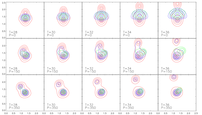
Figure 1.— Snapshots of merging galaxy clusters (infall velocity is upward) after the first core passage at time, $T$, in output time units (left to right), assuming different impact parameters, $P$ = 0, 150, and 350 kpc (from top to bottom). All other parameters held fixed (runs RM1V48p00, RM1V48p15, and RM1V48p35; see Table 1 for details). We show contour plots of projected mass surface density, X-ray emission and SZ contours (red, blue and green lines). The contour levels are chosen arbitrarily to make it easier to compare morphologies and avoid clutter. The collision is in the plane of the sky (the projection axis is in the line of sight). The images are 2.5 Mpc $\times$ 2.5 Mpc.

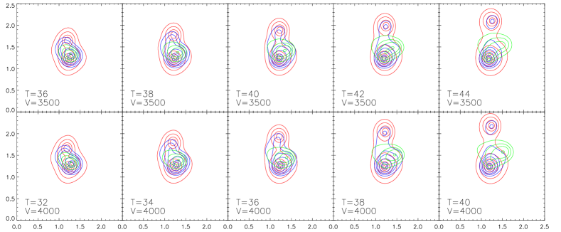
Figure 2.— Same as Figure 1 but assuming different initial relative velocities, 3500 and 4000, in unit of km s^-1 (from top to bottom), all other parameters held fixed (runs RM1V35p15 and RM1V40p15; see Table 1 for details of the simulations).

3.2. FLASH 3D Simulations

We have run a set of simulations of galaxy cluster mergers systematically changing the initial mass ratios, impact parameters, and relative velocities. In Table 1 we show the initial parameters for those runs we discuss in detail in our paper. In this table the first column is the identification number for our runs using the following convention: the numbers after M, V and P represent the mass of the second cluster in units of $10^{\,14}\,$ $\mbox{\rm M}_{\odot}$, the initial relative velocity in units of 100 $\rm km\,s^{-1}$, and the impact parameter in units of 10 kpc. The mass of the main cluster was assumed to be 2.1 $\times 10^{\,14}\,$$\mbox{\rm M}_{\odot}$, The concentration parameters were assumed to be 5 and 8 for the main and the infalling cluster. We have also run a few simulations with different gas mass fractions, concentration parameters and mass rations, and one simulation with higher resolution.

4. SZ, X-ray and Surface Mass Density Images

After the simulation finished, we generated SZ, X–ray and surface mass density, $\Sigma$, images assuming different viewing angles (expressed as rotation angles out of the plane of the sky) and phases (time elapsed after first core passage) of the collisions.

Since relativistic corrections are important in the high temperature shocked gas ($T_{g}\lower 3.0pt\hbox{$\hbox to0.0pt{\raise 5.0pt\hbox{$\char 62\relax$}\hss}\mathchar 29208\relax$}$ 30 keV), we generated SZ and X–ray images using relativistic corrections. We calculated the SZ surface brightness using

$$I_{SZ}\,(x,y)\propto\int_{\ell_{1}}^{\ell_{2}}\rho_{g}\,T_{g}\bigl{[}g(\nu)+\Sigma_{n=1}^{n=4}Y_{n}\,\Theta^{n}\bigr{]}\,d\ell,$$ (7)

where $\Theta=k_{B}T_{g}/(m_{e}c^{2})$ and $g(\nu)={\text{coth}}(x_{\nu}/2)-4$, $x_{\nu}=h_{P}\,\nu/(k_{B}T_{cmb})$, and $\nu$ is the frequency, $T_{cmb}$ is the temperature of the cosmic microwave background, $h_{P}$, $k_{B}$, $c$ and $m_{e}$, are the Planck and Boltzmann constants, the speed of light and the electron mass. The relativistic corrections, $Y_{1,2,3,4}$, were taken from Itoh, Kohyama & Nozawa (1998).

We generated the X–ray images using Rybicki & Lightman (1979)’s expression for the relativistic X-ray thermal bremsstrahlung,

$$I_{X}(x,y)\propto\int_{\ell_{1}}^{\ell_{2}}\rho_{g}^{2}\,T_{g}^{1/2}g_{ff}\,(1+4.4\times 10^{-10}T_{g})\;d\ell,$$ (8)

where the Gaunt factor, $g_{ff}=(2\sqrt{(}3)/\pi)[1+0.79\,(4.95\times 10^{5}/T_{g})]$ (see also Hughes & Birkinshaw 1998).

We integrated the total (dark matter and gas) density along the line of sight (LOS) from different viewing angles to obtain the mass surface density images at position, $x$ and $y$:

$$\Sigma_{X}(x,y)\propto\int_{\ell_{1}}^{\ell_{2}}\,(\rho_{d}+\rho_{g})\;d\ell,$$ (9)

where $\ell$ is the spatial coordinate in the LOS.

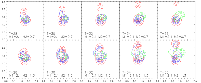
Figure 3.— Same as Figure 1 but assuming different mass rations: the mass of the main cluster was fixed at M₁ = 2.1, and the infalling cluster with masses: M₂ = 0.7 and 1.3 in unit of 10¹⁴ $\mbox{\rm M}_{\odot}$ (from top to bottom), all other parameters held fixed (see text for details).

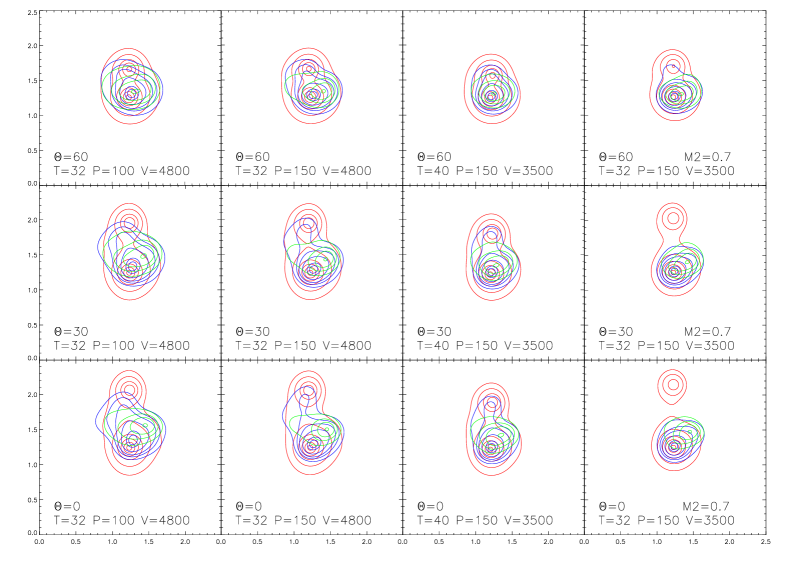
Figure 4.— Snap hots of mass surface density, SZ effect and X–ray images of merging clusters of galaxies as a function of different rotation angles, $\Theta$ = 0^∘, 30^∘, 60^∘(bottom to top), away from the main plane of the collision with axis perpendicular to the direction of the initial infalling velocity for different initial velocities. The color code is the same as in Figure 1. The infall velocity points upward. The initial masses are: $M_{1}=2.1$ $\times 10^{\,14}\,$$\mbox{\rm M}_{\odot}$, $M_{2}=1.0$ $\times 10^{\,14}\,$$\mbox{\rm M}_{\odot}$, except for the right column. From left to right: $P=100,150,150,150$ kpc, $V=4800,4800,3500,3500$ in km s^-1. All other parameters help fixed (see text for details). The images are 2.5 Mpc $\times$ 2.5 Mpc.

5. Results: Offsets Between the X-ray and SZ Centers

In this paragraph we discuss general aspects of our results. We have run simulations with different initial galaxy cluster masses and found similar dependence of the offsets between X-ray and SZ centers on different impact parameters and relative velocities. Thus we choose to show our results with fixed $M_{1}=2.1\times 10^{14}$ $\mbox{\rm M}_{\odot}$, since these give the best match with the observed morphology of CL0152-1357, which we will discuss in the next section. In Figure 1 we show snapshots of merging galaxy clusters after the first core passage assuming different impact parameters, $P=0$, 150 and 350 kpc, all other parameters of the simulations were held fixed (runs RM0p7V48P15 and RM1p3V48P15, see Table 1 for details of the simulations). The contour plots centered on the main cluster show the mass surface density, $\Sigma$, the X-ray emission and SZ contours (red, blue and green lines) projected to the main plane of the collision containing the two mass centers and the relative velocity vector (i.e., the collision is in the plane of the sky). $T$ represents the elapsed time in output file time units. The images are 2.5 Mpc $\times$ 2.5 Mpc.

The most obvious feature we recognize looking at Figure 1 is the different behavior of the infalling cluster gas and the most massive component, the dark matter. As we expected, the dark matter in the infalling cluster, due to its collisionless nature, simply passes through the main cluster smoothly, while the gas gets shocked because of the collision with the gas of the main cluster, and it is slowed down due to ram pressure. As a consequence, the gas of the infalling cluster will be out of equilibrium, and it gets displaced relative to the dark matter, it falls behind the center of the infalling cluster dark matter.

The effect of the ram pressure as a function of the impact parameter can be seen clearly. At larger impact parameters the core of the infalling cluster goes through less dense regions of the main cluster and, since the ram pressure is proportional to density $\times$ velocity², the infalling cluster retains more and more of its gas. The displacement between the SZ and X-ray peaks can be seen in all cases with non-zero impact parameter.

Figure 5.— SZ–X–ray offsets as a function of the distance between the dark matter mass centers of the two merging clusters for different initial relative velocities: 3000, 3500, 4000, 4500, and 4800 $\rm km\,s^{-1}$ (plus signs, stars, squares, triangles and diamonds connected by short dashed, dot-dashed, solid, long dashed, dot-dot-dot-dashed lines).

Figure 6.— Same as Figure 5 but for different impact parameters: P = 0, 150, 250, 350 kpc (stars, squares, triangles and diamonds connected by dot-dashed, solid, long dashed, dot-dot-dot-dashed lines). All other parameters help fixed (see Table 1 for details of the simulations).

We can see how the displacement depends on the initial relative velocity by studying Figure 2. In this figure we show results for $V=$ 3500 $\rm km\,s^{-1}$ and 4000 $\rm km\,s^{-1}$, all other parameters held fixed (runs RM1V35p15 and RM1V40p15; see Table 1 for details of the simulations). Results from simulations with the same initial conditions but with relative velocities of $V=$ 4800 $\rm km\,s^{-1}$ are shown in the second row of Figure 1. Again, we can see that assuming larger relative velocities, the infalling cluster can retain less of its gas due to ram pressure stripping. Also, larger velocities result larger displacements between the SZ and X–ray peaks. However, it seems that if the velocity is large enough, $\;\buildrel>\over{\sim}\;$3500 $\rm km\,s^{-1}$, we obtain large displacements, $\;\buildrel>\over{\sim}\;$200–300 kpc (the largest offset is at $T=40$ for this relative velocity).

In Figure 3 we show snapshots of the collisions as a function of different masses of the subcluster. The mass of the main cluster was fixed at $M_{1}=2.1\times 10^{14}$ $\mbox{\rm M}_{\odot}$, and the masses of the infalling cluster were $M_{2}$ = 0.7 and 1.3 $\times 10^{14}$ $\mbox{\rm M}_{\odot}$ (for $M_{2}$ = 1.0 see the second row of Figure 1, for which the other initial parameters are the same). Again, all other parameters held fixed (see Table 1 for details). In this case we see the result of two opposing effects: the ram pressure is striping the gas of the infalling cluster, and the gravity is trying to keep the gas, the relative velocities were held fixed. Assuming $M_{2}=0.7\times 10^{14}$ $\mbox{\rm M}_{\odot}$, the infalling cluster looses all its gas, and with increasing mass, the subcluster retains more and more of its gas ($M_{2}$ = 1, and 1.3 $\times 10^{14}$ $\mbox{\rm M}_{\odot}$).

In Figure 4, we show the projections rotated by angles $\Theta$ = 0^∘, 30^∘, 60^∘, away from the main plane of the collision with axis perpendicular to the direction of the initial infalling velocity (from bottom to top, runs RM1V48p10, RM1V48p15, RM1V35p15 and RM0p7V48P15). The infall velocity points upward. The initial masses are: $M_{1}=2.1$ $\times 10^{\,14}\,$$\mbox{\rm M}_{\odot}$, $M_{2}=1.0$ $\times 10^{\,14}\,$$\mbox{\rm M}_{\odot}$, except for the right column for which $M_{2}=0.7$ $\times 10^{\,14}\,$$\mbox{\rm M}_{\odot}$. From left to right: $P=100,150,150,150$ kpc, $V=4800,4800,3500,3500$ in km s^-1. All other parameters help fixed (see Table 1 for details). It is interesting to note the significant changes in SZ morphology, and, as a consequence, the offset between SZ and X–ray peaks: the offset gets smaller with larger rotation angle for all cases shown.

Figure 7.— Same as Figure 6 but for different initial mass ratios: M₁ = 2.1, fixed, M₂ = 0.7,1.0,1.3,1.6 in units of $10^{\,14}\,$$\mbox{\rm M}_{\odot}$ (stars, squares, triangles and diamonds connected by short dashed, dot-dashed, solid, long dashed, dot-dot-dot-dashed lines). The plus signs represent results from a higher resolution run with M${}_{1}=2.1\times$$10^{\,14}\,$$\mbox{\rm M}_{\odot}$ and M${}_{2}=1\times$$10^{\,14}\,$$\mbox{\rm M}_{\odot}$.

Figure 8.— Offsets between the two mass centers and the SZ and X–ray peaks (upper and lower set of curves) as a function of the cosine of the rotation angle away from the main plane of the collision with axis perpendicular to the direction of the initial infalling velocity for different impact parameters: 100, 150, 200, 250 kpc (stars, squares, triangles and diamonds connected by dot-dashed, solid, dashed, dot-dot-dot dashed lines).

We show our results for the offsets between the SZ and X-ray peaks for different initial velocities, impact parameters, and masses in Figure 5 (runs RM1V30p15, RM1V35p15, RM1V40p15, RM1V45p15, and RM1V48p15), Figure 6 (runs RM1V48p00, RM1V48p15, RM1V48p25, and RM1V48p35), and Figure 7 (runs RM0p7V48P15, RM1V48p15, RM1p3V48P15, and RM1p6V48P15).

A qualitative analysis of the offset between the SZ and X–ray peaks shows that 40$\arcsec$ or larger distances between the peaks can be produced as long as the relative velocities are at least 4000 $\rm km\,s^{-1}$ (see Figure 5). At large initial relative velocities (V = 4800 $\rm km\,s^{-1}$) runs with impact parameters between 100 and 250 kpc, or, with fixed P = 150 kpc, all masses with fixed M₁ = 2.1$\times 10^{\,14}\,$$\mbox{\rm M}_{\odot}$, and M₂ = 0.7–1.6$\times 10^{\,14}\,$$\mbox{\rm M}_{\odot}$, the offset is larger than 40$\arcsec$ (see Figures 6 and 7).

We have carried our a run using higher resolution to check if our resolution is high enough. The offsets for this run are included in our Figure 7 (plus signs). In this figure, the squares represent offsets based on a run we used in all simulations. The two offsets are almost identical, thus we conclude that our resolution is sufficient for our purpose.

In Figure 8 we illustrate how the offsets between the SZ and X–ray change with rotation angle (out of the plane of the collision), $\Theta$, for different impact parameters, P = 100, 150, 200, 250 kpc (runs RM1V48p10, RM1V48p15, RM1V48p20 and RM1V48p25). The upper lines represent the distances between the two mass peaks, the lower lines show the offsets between the SZ and X–ray peaks. Assuming $\Theta=0$, we find large distances between the projected mass centers, about 110$\arcsec$, when the largest offset between the SZ and X–ray peaks are about 40$\arcsec$. At each $\Theta$, the largest offset we obtain is for $P=$ 150 kpc, $M_{1}=2.1$ $\times 10^{\,14}\,$$\mbox{\rm M}_{\odot}$, $M_{2}=1.0$ $\times 10^{\,14}\,$$\mbox{\rm M}_{\odot}$, and $V=$ 4800 $\rm km\,s^{-1}$. This is the largest offset for all masses we considered here.

We conclude that large relative velocities of $V$ $\;\buildrel>\over{\sim}\;$4000 $\rm km\,s^{-1}$ with different impact parameters close to the core radius, and masses can easily produce 40$\arcsec$, or larger offset between SZ and X–ray peaks.

6. Application to Galaxy Cluster CL0152-1357

In this section we use our results from FLASH simulations to interpret multi-wavelength observations of the galaxy cluster CL0152-1357. We use the morphology of the X-ray, SZ and $\Sigma$ images, and the offsets between the SZ and X–ray peaks as well as the distances between the mass peaks of the two components to constrain the initial conditions of the collision. We also discuss the implications of our results for CL0152-1357 as a test for $\Lambda$CDM and the effect of SZ resolution on the interpretation of galaxy clusters.

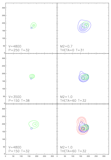
Figure 9.— Contours of SZ, X-ray and mass surface density (green, blue, red colors) for different models. Left column: similar SZ morphology to the observed (to aid the eye, we included the center of the X-ray emission) with different initial velocities, 3500, 4800 in units of $\rm km\,s^{-1}$, and impact parameters (150 kpc and 250 kpc). Right column: top 2 panels: SZ and X-ray morphology similar to the observed, bottom panel: SZ, X-ray and mass surface density morphology similar to the observed (60^∘ rotation away form the plane of the collision). The contour levels are chosen arbitrarily to make an easy comparison to the observed morphology. The images are $350\,\arcsec\times 350\,\arcsec$.

6.1. Constraining Initial Conditions

The ATC SZ image of CL0152-1357 seems to be nearly circularly symmetric (see Figure 1 of Massardi et al. 2010). Searching for similar SZ morphology in our projected images we find candidates with different impact parameters and initial relative velocities (see green contours in the left column of Figure 9, results for runs RM1V48p25, RM1V35p15 and RM1V48p15), also with different initial masses (green contours in first panel in Figure 9, run RM0p7V48P15 with $M_{1}$ = 2.1 $\times 10^{\,14}\,$$\mbox{\rm M}_{\odot}$ and $M_{1}$ = 0.7 $\times 10^{\,14}\,$$\mbox{\rm M}_{\odot}$ (see Table 1 for other parameters). We assumed a 35$\arcsec$ resolution for SZ observations (ATCA), and choose the contours to reflect the signal observed using ATCA (Figure 1 of Massardi et al. 2010). For comparison, we also plot the centers of the X–ray emission to show that, in all of these cases, there is an offset between the SZ and X–ray peaks. These panels illustrate that an observed nearly circular SZ distribution, with the assumed SZ sensitivity and resolution, can not be used to identify a shock in a cluster, nor can the initial conditions be constrained using only SZ observations if we know that there is a shock. It is clear that we need a multi-frequency approach in this case.

Including the observed SZ and X–ray morphology of CL0152-1357 (Figure 1 of Massardi et al. 2010 and Figure 3 of Maughan et al. 2006) to constrain the initial conditions, we find that the best match with observations is provided by run RM0p7V48P15 with masses of 2.1 $\times 10^{\,14}\,$$\mbox{\rm M}_{\odot}$ and 0.7 $\times 10^{\,14}\,$$\mbox{\rm M}_{\odot}$, and $\Theta=0$ (the collision in the pane of the sky), P = 150 kpc, and initial relative velocity 4800 $\rm km\,s^{-1}$ (top panel in the right column of Figure 9). We assumed a 12$\arcsec$ X–ray resolution (XMM-Newton). This high velocity seems to be needed to obtain the large offset, about 45$\arcsec$ between the SZ and X-ray peaks, and the observed SZ and X-ray morphology. Allowing for some uncertainty in the relative pointing between the SZ and X-ray instruments, we find a good match with observations for run RM1V48p15 with 2.1 $\times 10^{\,14}\,$$\mbox{\rm M}_{\odot}$ and 1 $\times 10^{\,14}\,$$\mbox{\rm M}_{\odot}$, and the same impact parameter and relative velocity as the previous run (middle panel in the right column of Figure 9). This run with a rotation angle of $\Theta=60$^∘can also reproduces the observed SZ and X-ray morphology, but the SZ and X-ray offset is only about 20$\arcsec$. Note, that the relative coordinate positions of the SZ and X–ray peaks differ for these two cases, but that can not be observed using these two wavelengths because we do not know the original orientation of the two clusters. Even though the possible initial configurations are more restricted by using X–ray and radio observations, we can conclude that, using morphology, these observations are not sufficient to confine the initial conditions of the collision.

We include now the mass surface density map of CL0152-1357 derived from gravitational lensing observations in our analysis assuming a resolution of 20$\arcsec$ (Jee et al., 2005). The importance of the lensing observations is that the distance between the two dark matter centers constrain the phase of the collision, i.e. the time elapsed since the first core passage (subject to projection effects). Having some constraints on the time elapsed since the first core passage and the X–ray and SZ morphology enable us to put more constraints on the initial conditions of the collision.

We are looking for an offset between the SZ and X–ray peaks of about 45$\arcsec$, and a distance of about 50$\arcsec$ between the mass peaks, in projection. For all projections perpendicular to the main plane of the collision ($\Theta=0$$\arcsec$), the distance between the mass peaks are around 100$\arcsec$–120$\arcsec$, so we need to rotate the infalling cluster center towards the line of sight, thus we conclude that the rotation angle, $\Theta$, should be greater than zero. We find that, with $\Theta$ = 60^∘, our run RM1V48p15 with P = 150 kpc, M₁ = 2.1$\times 10^{\,14}\,$$\mbox{\rm M}_{\odot}$, M₂ = 1$\times 10^{\,14}\,$$\mbox{\rm M}_{\odot}$, and V = 4800 $\rm km\,s^{-1}$, provides the best fit to all three observations. The morphology of this model is close to the observed SZ and X–ray morphologies (Massardi et al., 2010; Maughan et al., 2006), and the distance between the projected mass centers is the same as the observed (Jee et al., 2005). It is encouraging that these masses are similar to the masses derived for these components by (Jee et al., 2005). We were running simulations with larger masses (M${}_{1}>$ 2.1$\times 10^{\,14}\,$$\mbox{\rm M}_{\odot}$), but the resulting X–ray morphologies did not match the observations. The offset between the SZ and X–ray peaks is less than the observed 45$\arcsec$. This difference may be caused by absolute calibration for the positions between the ACT and XMM-Newton. However, it is also possible that the lensing observations have some systematics. Gravitational lensing observations are very difficult, and the mass surface density reconstruction depends strongly on the assumed priors. Compare, for example, the results using different priors for reconstruction of the mass surface density for RX J1347.5–1145 (see Figure 4 of Miranda et al. 2008). It would be useful to have mass surface density reconstructions using different methods to check for systematics in the analysis of CL0152-1357.

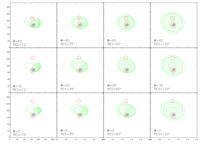
Figure 10.— Projected mass surface density, X-ray emission and SZ contours red, blue and green contours) of run RM1V48p15 (see Table 1) as a function of rotation angle, $\Theta$, away from the plane of the collision for different resolutions, FWHM, of the SZ observations: FWHM = 10$\,\arcsec$, 35$\,\arcsec$, 60$\,\arcsec$, and 120$\,\arcsec$ (left to right). The rotation angles are: $\Theta$ = 0^∘, 30^∘, 60^∘ away from main plane of the collision (from bottom to top). The images are $350\,\arcsec\times 350\,\arcsec$.

6.2. Tests for $\Lambda$CDM

Merging galaxy clusters can provide tests for our most successful cosmological scenario, the $\Lambda$CDM models many ways. The features of mergers predicted by $\Lambda$CDM models, for example, can be compared to those derived from observations (Forero-Romero et al., 2010; Mastropietro & Burkert, 2008).

Forero-Romero et al. (2010) derived the distribution of the offsets between dark matter (DM) and gas centers of galaxy clusters drawn from one of the largest non-radiative, $\Lambda$CDM cosmological simulations using SPH, usually referred to as the MareNostrum Universe. They found that the distribution of the 2D offsets between the DM and gas density peaks of the bullet cluster would have a probability of 1%–2% from simulations. Thus they concluded that it is possible to reproduce the observed offset between DM and gas density peaks as large as observed in the bullet cluster assuming $\Lambda$CDM cosmology.

The estimated initial relative velocities of clusters can also be used as a test for $\Lambda$CDM models. Mastropietro & Burkert (2008) carried out galaxy cluster merger simulations and found that their best model requires a relative initial velocity of 3000 $\rm km\,s^{-1}$ for the “bullet” cluster, 1E0657-56. However, they concluded that the probability of finding such a high relative velocity given their best model is less then 0.5%. We found a relative velocity of 4800 $\rm km\,s^{-1}$ for our best model for CL0152-1357. The median relative velocity of a galaxy cluster with about the total mass of CL0152-1357 (Jee et al., 2005), $M_{1}$ = 5 $\times 10^{\,14}\,$$\mbox{\rm M}_{\odot}$, is about 1500 $\rm km\,s^{-1}$ (Hayashi & White, 2006). The infall velocity of our best model is about three times the value of our best fit model. Based on the results of Hayashi & White (2006), this relative velocity is very unlikely in a $\Lambda$CDM model. These results suggest that there is a mismatch between the initial relative velocities derived from simple idealized cluster merging simulations and those derived from $\Lambda$CDM simulations. There are two possibilities: either our simple cluster models or our $\Lambda$CDM models are missing some important physics. A detailed analysis of the origin of this mismatch is out of the scope of our paper, we are going to address this question in a future paper.

6.3. The Effect of SZ Resolution

When using clusters to derive cosmological parameters we assume that they are relaxed. The statistical methods use scaling relations derived based on relaxed clusters, individual methods assume relaxed clusters to derive their physical parameters. Both statistical and individual methods may be biased due to the fact that some clusters are not relaxed. Statistical methods might have to be corrected for this effect, when using individual methods, we can just simply exclude non-relaxed clusters. Some of these aspects of SZ resolution and the importance of high-resolution SZ observations were discussed in Korngut et al. (2010); Mason et al. (2010); Massardi et al. (2010) for example.

In this paper we discuss some aspects of the identification of non-relaxed clusters focusing on SZ observations. The effect of non-relaxed clusters to determining cosmological parameters using SZ observations was discussed in Wik et al. (2008). The new generation of ground based SZ telescopes have a very large span in resolution, from about 10$\arcsec$ to 3$\arcmin$.

We illustrate the importance of high resolution SZ observation in identifying merging clusters in Figure 10. As an example, we use the best model we found for CL0152-1357. In this Figure we show snapshots for this model after the first core passage using different SZ resolution (green contours). We also plot the centers of projected mass (red contours) and X–ray peak (blue contours). From this Figure we can see that, with high resolution, 10$\arcsec$–35$\arcsec$, SZ observations would be sufficient to identify the merger based on its disturbed morphology. Having also X–ray observations would help us because we can use the offset between the SZ and X–ray peaks. In the case when the collision is in the plane of the sky ($\theta=0$), this offset is about 50$\arcsec$ with high SZ resolution, and about 40$\arcsec$ for low, 1$\arcmin$– 2$\arcmin$ resolution. In this case the offset is observable assuming a better than 40$\arcsec$ absolute pointing calibration for the SZ telescope, which is a reasonable assumption. However, if the rotation angle is large, say 60^∘, high resolution SZ instruments still measure an about 40$\arcsec$ offset between the SZ and X–ray peaks, but with lower resolution, we obtain an only 10$\arcsec$ offset, which is close or less then the absolute pointing calibration of SZ instruments. Therefore, we conclude that with an SZ resolution of about 10$\arcsec$ and 35$\arcsec$, GBT/Mustang and ATCA have the sufficient resolution to identify this merger, but using lower resolution instruments of 1$\arcmin$or 2$\arcmin$, BOLOCAM and AMiBA, will not be able to identify the merger. We could identify the merger in any case if we have not only SZ and X–ray measurements, but also surface mass density maps from lensing optical/infrared (optical/IR) observations.

Our results suggest that if we want to identify mergers, we should use either high resolution SZ observations, or multi–frequency observations. In any case, galaxy cluster observations with low resolution SZ instruments with large field of view are still useful because they can be potentially used to constrain the large scale distribution of the intra-cluster gas (e.g., Molnar et al. 2010).

7. Conclusion

We have been studying galaxy cluster merging using self-consistent 3D N-body/hydrodynamical simulations of idealized clusters. We have found that significant offsets results between the X–ray and SZ peaks ($\hbox to0.0pt{\raise 5.0pt\hbox{$\char 62\relax$}\hss}\mathchar 29208\relax$ 40 $\arcsec$) if the relative velocities are equal or larger than about 4000 $\rm km\,s^{-1}$. This offset can be observed using an SZ instrument with high sensitivity and high angular resolution (at least about 10$\arcsec$–35$\arcsec$), in which case the merging cluster can be identified using SZ observations only (Figure 10). However, using multi-frequency observations seems to be a more practical way to identify merging galaxy clusters.

We have applied numerical simulations to interpret multi-frequency observations, radio (SZ), X–ray and optical/IR (lensing reconstruction) of CL0152-1357. We have found that the offsets between the SZ and X–ray peaks provide important constraints on the initial parameters of the merging clusters, the offsets between the two peaks of the mass surface densities provide constraints on the phase of the collision (i.e., the time elapsed after the first core passage), and that the SZ peak coincides with the peak in the pressure times the characteristic length in the line of sight and not the pressure maximum (as it does for clusters in equilibrium). The peak in the X–ray emission, as expected, coincides with the density maximum of the main cluster. As a consequence, the morphology of the SZ signal, and therefore the offset between the SZ and X-ray peaks, change with viewing angle.

We conclude that analyzing the morphology of SZ, X–ray, and surface mass density images based on multi-frequency observations (radio, X–ray and optical/IR) enables us to put meaningful constraints on the masses of the colliding clusters, the impact parameter and initial relative velocity of the collision.

References

- Agertz et al. (2007) Agertz, O., et al. 2007, MNRAS, 380, 963
- Allen, Evrard & Mantz (2011) Allen, S. W., Evrard, A. E., & Mantz, A. B. 2011, arXiv:1103.4829v1 [astro-ph.CO]
- Allen et al. (2008) Allen, S. W., Rapetti, D. A., Schmidt, R. W., Ebeling, H., Morris, R. G., & Fabian, A. C. 2008, MNRAS, 383, 879
- Angrick & Bartelmann (2011) Angrick C., & Bartelmann, M., 2011, arXiv:1102.0458v1 [astro-ph.CO]
- Bonamente et al. (2006) Bonamente, M., Joy, M. K., LaRoque, S. J., Carlstrom, J. E., Reese, E. D., & Dawson, K. S. 2006, ApJ, 647, 25
- Borgani et al. (2001) Borgani, S., et al. 2001, ApJ, 561, 13
- Bryan & Norman (1998) Bryan, G. L., & Norman, M. L. 1998, ApJ, 495, 80
- Del Popolo et al. (2010) Del Popolo, A., Costa, V., & Lanzafame, G. 2010, A&A, 514, A80
- Ettori et al. (2009) Ettori, S., Morandi, A., Tozzi, P., Balestra, I., Borgani, S., Rosati, P., Lovisari, L., & Terenziani, F. 2009, A&A, 501, 61