Numerical solution of nonlocal hydrodynamic Drude model
for arbitrary shaped nano-plasmonic structures
using Nédélec finite elements

Abstract

Nonlocal material response distinctively changes the optical properties of nano-plasmonic scatterers and waveguides. It is described by the nonlocal hydrodynamic Drude model, which – in frequency domain – is given by a coupled system of equations for the electric field and an additional polarization current of the electron gas modeled analogous to a hydrodynamic flow. Recent attempt to simulate such nonlocal model using the finite difference time domain method encountered difficulties in dealing with the grad-div operator appearing in the governing equation of the hydrodynamic current. Therefore, in these studies the model has been simplified with the curl-free hydrodynamic current approximation; but this causes spurious resonances. In this paper we present a rigorous weak formulation in the Sobolev spaces $H(\mathrm{curl})$ for the electric field and $H(\mathrm{div})$ for the hydrodynamic current, which directly leads to a consistent discretization based on Nédélec’s finite element spaces. Comparisons with the Mie theory results agree well. We also demonstrate the capability of the method to handle any arbitrary shaped scatterer.

1 Introduction

Dispersive material properties play an important role in the light-matter interactions in plasmonic structures. For this quite often the Drude model and the Lorentz material model are used [1], which take into account spatially purely local interactions between electrons and the light. In recent investigation it has been found that these local models are inadequate as the size of the plasmonic scatterers become much smaller than the wavelength of the incident light [2, 3]. To overcome this, a sophisticated nonlocal material model is required, such as the hydrodynamic model of the electron gas as discussed by Boardman et al. [4].

In the first principle formulation, the hydrodynamic model of the electron gas is formulated by coupling macroscopic time domain Maxwell’s equations for electromagnetic fields with the equations of motion of the electron gas which behaves similar to hydrodynamic flow [4]. This gives rise to a hydrodynamic polarization current. The resultant coupled system of equations is flexible enough to incorporate a variety of advanced quantum mechanical effects. When considered only the kinetic energy of the free electrons, it yields the nonlocal hydrodynamic Drude model (discussed in Sec. 2).

In one of the earlier attempts, the nonlocal hydrodynamic Drude model has been simulated with the finite difference time domain (FDTD) method, but with the quasi-static approximation [5]. As a consequence of this approximation, the tensorial grad-div operator ($\nabla(\nabla\cdot\boldsymbol{A})$) appearing in the governing equation for the hydrodynamic current simplifies to vectorial linear Laplacian operator ($\nabla^{2}\boldsymbol{A}$). This was needed to render the system into a form suitable for the standard FDTD framework. However the comparison with the analytical Mie theory [2] showed that this approach produces spurious plasmonic resonances below the plasma frequency [6].

In this paper we do not rely on the quasi-static approximation, and we present a rigorous weak formulation in the frequency domain (with time dependence $\exp{(-i\omega t)}$ and for a typical light scattering setting as shown in Fig. 1), which directly allows a consistent discretization within Nédélec finite element spaces. We would like to point out that while the present work was under review, Toscano et al. have independently reported a finite element approach for the simulation of the nonlocal hydrodynamic Drude model [7]. While the emphasis of their work is on analyzing physical effects due to the nonlocality, the main contribution of this work is to present appropriate finite element framework behind such computational scheme (see Sec. 3). This will ensure that the finite element solutions are physically meaningful.

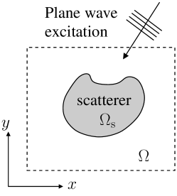
Figure 1: Scattering setting: A plane wave of angular frequency $\omega$ is incident on a nano-plasmonic scatterer with nonlocal material properties and arbitrary shaped domain $\Omega_{\mathrm{s}}$. The scattering problem is defined on the entire space, but for numerical computations we restrict it to a finite (computational) domain $\Omega$, which necessitates construction of transparent boundary conditions (e.g. perfectly matched layer). We assume a homogeneous medium outside $\Omega$.

The paper is organized as follows. Sec. 2 introduces the nonlocal hydrodynamic Drude model, various approximations involved in it, and derives the governing coupled system of equations for the electric field and the nonlocal hydrodynamic current. A finite element formulation for the governing equation of the electric field follows the standard procedure based on the curl conforming elements (as in the case of the usual local material models [8]), but one needs to choose an appropriate finite element space for solution of the equation for the hydrodynamic current. We discuss this consistent weak formulation and the finite element setting of the model in Sec. 3. Then in Sec. 4 we validate the simulation results of this model with analytical Mie theory results. We also demonstrate the ability of the method to handle arbitrary shaped geometry with the example of V groove channel plasmon-polariton devices.

2 Nonlocal hydrodynamic Drude model

For the sake of clarity and to highlight various approximations involved in the nonlocal hydrodynamic Drude model, we derive its governing equations in this section. The macroscopic Maxwell’s equations for non-magnetic materials with no external current density density and no external charge density are

$$\nabla\times\boldsymbol{E}(\boldsymbol{r},\omega) = i\omega\mu_{0}{\boldsymbol{H}}(\boldsymbol{r},\omega),$$ (1)

$$\nabla\times\boldsymbol{H}(\boldsymbol{r},\omega) = -i\omega\varepsilon_{0}\varepsilon_{\mathrm{loc}}(\boldsymbol{r},\omega)\boldsymbol{E}(\boldsymbol{r},\omega)+\boldsymbol{J}_{\mathrm{HD}}(\boldsymbol{r},\omega),$$ (2)

$$\nabla\cdot\boldsymbol{D}(\boldsymbol{r},\omega) = -en(\boldsymbol{r},\omega),$$ (3)

$$\nabla\cdot\boldsymbol{B}(\boldsymbol{r},\omega) = 0,$$ (4)

where $\boldsymbol{E}$ is the electric field, $\boldsymbol{H}$ is the magnetic field, $\boldsymbol{D}=\varepsilon_{0}\varepsilon_{\mathrm{loc}}\boldsymbol{E}$ is the electric displacement, and $\boldsymbol{B}=\mu_{0}\boldsymbol{H}$ is the magnetic induction. $\varepsilon_{0}$ is the permittivity constant and $\mu_{0}$ is the permeability constant. A part of the relative permittivity due to the local-response is defined as $\varepsilon_{\mathrm{loc}}=\varepsilon_{\infty}(\boldsymbol{r})+\varepsilon_{\mathrm{inter}}(\boldsymbol{r},\omega)$. $\varepsilon_{\infty}$ is the relative permittivity for infinite frequency. If the material system under consideration has interband transitions, then the corresponding relative permittivity (typically described by the Lorentz material model) is given by $\varepsilon_{\mathrm{inter}}$.

The effect of nonlocal material response on plasmonic scatterers is incorporated by an auxiliary nonlocal hydrodynamic current density $\boldsymbol{J}_{\mathrm{HD}}$. This polarization current is defined only on the spatial domain $\Omega_{\mathrm{s}}$ where the plasmonic scatterer exists, and set to zero outside it. The exact material interface conditions for $\boldsymbol{J}_{\mathrm{HD}}$ are discussed later on. The current density $\boldsymbol{J}_{\mathrm{HD}}$ is related with the electron gas density $n$ by

$$\boldsymbol{J}_{\mathrm{HD}}(\boldsymbol{r},\omega)=-en(\boldsymbol{r},\omega)\boldsymbol{v}(\boldsymbol{r},\omega),$$ (5)

where $e$ is the charge of the electron. In time domain, the hydrodynamic velocity $\boldsymbol{v}$ is related with the electron gas density $n$ by the continuity equation $\frac{\partial n(\boldsymbol{r},t)}{\partial t}+\nabla\cdot{(n(\boldsymbol{r},t)\boldsymbol{v}(\boldsymbol{r},t))}=0$. Let $n_{0}$ be the constant equilibrium density of the electron gas, and $n_{1}$ be the linear perturbation, then the time dependent density $n$ is written as $n(\boldsymbol{r},t)=n_{0}+n_{1}(\boldsymbol{r},t)$. Note that $n_{0}$ and $n_{1}$ are nonzero only in $\Omega_{\mathrm{s}}$. With this linearization ansatz, a term $\nabla\cdot{(n_{1}(\boldsymbol{r},t)\boldsymbol{v}(\boldsymbol{r},t))}$ is negligible, and the continuity equation in frequency domain simplifies to

$$-i\omega n_{1}(\boldsymbol{r},\omega)+n_{0}\nabla\cdot{\boldsymbol{v}(\boldsymbol{r},\omega)}=0.$$ (6)

The hydrodynamic velocity $\boldsymbol{v}(\boldsymbol{r},\omega)$ obeys the generalized momentum equation derivable from quantum mechanical Hamiltonian [4], which in frequency domain is given by

$$m_{\mathrm{e}}\left(-i\omega+{\boldsymbol{v}}\cdot{\nabla}\right)\boldsymbol{v}=-e(\boldsymbol{E}+{\boldsymbol{v}}\times{\boldsymbol{B}})-m_{\mathrm{e}}\gamma\boldsymbol{v}-\nabla\left(\frac{\delta g[n]}{\delta n}\right),$$ (7)

where $m_{\mathrm{e}}$ is the effective electron mass, $\gamma$ is the damping constant (= inverse of the collision time) and $g[n]$ is energy functional of the fluid.

Several further approximations are introduced in order to deal with Eq. (7). Assume that the nonlinear term corresponding to the hydrodynamic total derivative $({\boldsymbol{v}}\cdot{\nabla})\boldsymbol{v}$ is negligible. Also, the driving force of the electron fluid is only the electric field $\boldsymbol{E}$, and therefore we neglect the effect of the magnetic induction field $\boldsymbol{B}$. For the free electron gas, assume only the kinetic energy constitute $g[n]$ (neglecting the exchange and the correlation effects) [4], and along with Eq. (6) one can estimate

$$\nabla{\left(\frac{\delta g[n]}{\delta n}\right)}\approx m_{\mathrm{e}}\beta^{2}\frac{1}{n_{0}}\nabla{n_{1}}=m_{\mathrm{e}}\beta^{2}\frac{1}{i\omega}\nabla{(\nabla\cdot{\boldsymbol{v}(\boldsymbol{r},\omega)})},$$ (8)

with $\beta^{2}=\frac{3}{5}v_{\mathrm{F}}^{2}$ is a term proportional to the Fermi velocity $v_{\mathrm{F}}$ (here the value of the constant of proportionality is taken as $3/5$, but to be precise, it depends on the various properties of the physical setting under consideration [4]).

With these approximations Eq. (7) gives

$$\beta^{2}\nabla{(\nabla\cdot{\boldsymbol{v}(\boldsymbol{r},\omega)})}+\omega(\omega+i\gamma)\boldsymbol{v}(\boldsymbol{r},\omega) = -i\omega\frac{e}{m_{\mathrm{e}}}\boldsymbol{E}(\boldsymbol{r},\omega).$$

Multiplying this equation by $-en_{0}$, we get the governing equation for the nonlocal hydrodynamic current density $\boldsymbol{J}_{\mathrm{HD}}$

$$\beta^{2}\nabla{(\nabla\cdot{\boldsymbol{J}_{\mathrm{HD}}(\boldsymbol{r},\omega)})}+\omega(\omega+i\gamma)\boldsymbol{J}_{\mathrm{HD}}(\boldsymbol{r},\omega) = i\omega\omega_{\mathrm{p}}^{2}\varepsilon_{0}\boldsymbol{E}(\boldsymbol{r},\omega),\leavevmode\nobreak\$$ (9)

where $\omega_{\mathrm{p}}^{2}=\frac{e^{2}n_{0}}{\varepsilon_{0}m_{\mathrm{e}}}$ is the plasma frequency of the free electron gas. In this equation the macroscopic electric field $\boldsymbol{E}$ acts as a source for evolution of the hydrodynamic current. In turn, this hydrodynamic current influences the evolution of the electric field $\boldsymbol{E}$. This part of the model is obtained by taking curl of (1), and using (2), and then rearranging, we get the familiar curl-curl equation for $\boldsymbol{E}$ as

$$\nabla\times\mu_{0}^{-1}(\nabla\times\boldsymbol{E}(\boldsymbol{r},\omega))-\omega^{2}\varepsilon_{0}\varepsilon_{\mathrm{loc}}(\boldsymbol{r},\omega)\boldsymbol{E}(\boldsymbol{r},\omega)=i\omega\boldsymbol{J}_{\mathrm{HD}}(\boldsymbol{r},\omega).$$ (10)

Eq. (9) and (10) are the required coupled system of equations for the nonlocal hydrodynamic Drude model. Eq. (10) is defined on unbounded domain, but for numerical computations, it is restricted to a finite computational domain $\Omega$ by the transparent boundary condition like the perfectly matched layer. Whereas Eq. (9) is solved on the region $\Omega_{\mathrm{s}}$ containing the material with the nonlocal response, and outside it $\boldsymbol{J}_{\mathrm{HD}}=0$. Since the normal component of $\boldsymbol{J}_{\mathrm{HD}}$ is continuous across the material interfaces, it leads to ${\boldsymbol{n}}\cdot{\boldsymbol{J}_{\mathrm{HD}}}=0$ on the material interfaces.

Curl-free approximation: Using the vector calculus identity $\nabla{(\nabla\cdot{\boldsymbol{A}})}=\nabla\times{\nabla\times{\boldsymbol{A}}}+\nabla^{2}{\boldsymbol{A}}$, and assuming $\nabla\times{\boldsymbol{J}_{\mathrm{HD}}}=0$, Eq. (9) becomes

$$\beta^{2}\nabla^{2}{\boldsymbol{J}_{\mathrm{HD}}}(\boldsymbol{r},\omega)+\omega(\omega+i\gamma)\boldsymbol{J}_{\mathrm{HD}}(\boldsymbol{r},\omega)=i\omega\omega_{\mathrm{p}}^{2}\varepsilon_{0}\boldsymbol{E}(\boldsymbol{r},\omega).$$

This is precisely the frequency domain representation of the corresponding time domain equation, which is solved in Ref. [5, Eq. 14].

3 Weak formulation

In this section we bring the light scattering problem of Fig. 1 into a variational form. We start with Eq. (10) for the electric field, for which the weak formulation follows the standard procedure based on Nédélec’s curl conforming finite elements [8, 9]. An appropriate ansatz space for the electric field is the Sobolev space

$$H(\mathrm{curl},\Omega)=\left\{\boldsymbol{E}\in(L^{2}(\Omega))^{3}\,|\,\nabla\times{\boldsymbol{E}}\in(L^{2}(\Omega))^{3}\right\},$$

which contains fields with weakly defined curl-operator defined on the domain $\Omega$ [10, Sec. 3.5].

Multiply Eq. (10) with a trial function $\varphi\in H(\mathrm{curl},\Omega)$, and integrate over $\Omega$. Then partial integration yields

$$\int_{\Omega}\left((\nabla\times{\varphi})\cdot(\mu_{0}^{-1}\nabla\times{\boldsymbol{E}})-\omega^{2}\varphi\cdot\varepsilon_{\mathrm{loc}}\boldsymbol{E}\right)\,dV+\int_{\partial\Omega}\varphi\cdot(\boldsymbol{n}\times(\mu_{0}^{-1}\nabla\times{\boldsymbol{E}}))\,dA=i\omega\int_{\Omega}\varphi\cdot\boldsymbol{J}_{\mathrm{HD}}\,dV,$$ (11)

with the local permittivity $\varepsilon_{\mathrm{loc}}$ and with the outer normal $\boldsymbol{n}$ of the computational domain. At this stage, we encounter the problem of defining boundary conditions of the electric field on $\partial\Omega$, which is addressed by the transparent boundary condition. This can be realized in various forms like perfectly matched layers, infinite element method, etc. [10, Ch. 13]; but here, for the notational simplicity we will make use of the Dirichlet to Neumann (DtN) operator [11] (also known as the Calderon map approach [10, Sec. 9.4]).

Outside the scatterer the electric field is a superposition of the exciting (incoming) field $\boldsymbol{E}_{\mathrm{inc}}$ and the scattered field $\boldsymbol{E}_{\mathrm{s}},$ i.e. $\boldsymbol{E}=\boldsymbol{E}_{\mathrm{inc}}+\boldsymbol{E}_{\mathrm{s}}.$ The outward radiating scattered field satisfies Maxwell’s equations in the exterior domain, and the Silver-Müller radiation condition at infinity. But then $\boldsymbol{E}_{\mathrm{s}}$ is already defined by it’s Dirichlet field values on $\partial\Omega.$ Especially, one is able to determine the Neumann field values $\boldsymbol{n}\times(\mu_{0}^{-1}\nabla\times{\boldsymbol{E}_{\mathrm{s}}})|_{\partial\Omega}$ from $\boldsymbol{E}_{\mathrm{s}}|_{\partial\Omega}$. This mapping defines the so called DtN-operator. For the above Neumann boundary term we get

$$\int_{\partial\Omega}\varphi\cdot(\boldsymbol{n}\times(\mu_{0}^{-1}\nabla\times{\boldsymbol{E}}))\,dA = \int_{\partial\Omega}\varphi\cdot(\boldsymbol{n}\times(\mu_{0}^{-1}\nabla\times{(\boldsymbol{E}_{\mathrm{inc}}+\boldsymbol{E}_{\mathrm{s}})}))\,dA$$

$$= \int_{\partial\Omega}\varphi\cdot(\boldsymbol{n}\times(\mu_{0}^{-1}\nabla\times{\boldsymbol{E}_{\mathrm{inc}}}))\,dA+\int_{\partial\Omega}\varphi\cdot\mathrm{DtN}(\boldsymbol{E}_{\mathrm{s}})\,dA.$$

Using $\boldsymbol{E}=\boldsymbol{E}_{\mathrm{inc}}+\boldsymbol{E}_{\mathrm{s}}$ once more, we can eliminate the scattered field and recast Eq. (11) to

$$\int_{\Omega}((\nabla\times{\varphi})\cdot(\mu_{0}^{-1}\nabla\times{\boldsymbol{E}})-\omega^{2}\varphi\cdot\varepsilon_{\mathrm{loc}}\boldsymbol{E})\,dV + \int_{\partial\Omega}\varphi\cdot\mathrm{DtN}(\boldsymbol{E})\,dA-i\omega\int_{\Omega}\varphi\cdot\boldsymbol{J}_{\mathrm{HD}}\,dV$$

$$=-\int_{\partial\Omega}\varphi\cdot(\boldsymbol{n}\times(\mu_{0}^{-1}\nabla\times{\boldsymbol{E}_{\mathrm{inc}}}))\,dA + \int_{\partial\Omega}\varphi\cdot\mathrm{DtN}(\boldsymbol{E}_{\mathrm{inc}})\,dA,\;\forall\leavevmode\nobreak\ \varphi\in H(\mathrm{curl},\Omega),{}{}$$ (12)

where only the exciting field $\boldsymbol{E}_{\mathrm{inc}}$ appears on the right hand side.

It remains to bring the Eq. (9) for the hydrodynamic current into variational form. The subsequent weak formulation reveals that for a physically meaningful solution, the required ansatz space for $\boldsymbol{J}_{\mathrm{HD}}$ needs to be divergence conforming, which can be precisely realized by the Nédélec’s divergence conforming finite elements [9]. Thus the appropriate ansatz space for weak formulation of Eq. (9) is the Sobolev space

$$H_{0}(\mathrm{div},\Omega_{\mathrm{s}})=\left\{\boldsymbol{J}_{\mathrm{HD}}\in(L^{2}(\Omega_{\mathrm{s}}))^{3}\,|\,\nabla\cdot{\boldsymbol{J}_{\mathrm{HD}}}\in(L^{2}(\Omega_{\mathrm{s}}))^{3},\;\boldsymbol{n}\cdot\boldsymbol{J}_{\mathrm{HD}}=0\;\mbox{on}\;\partial\Omega_{\mathrm{s}}\right\}.$$

This restricts the hydrodynamic current to the plasmonic scatterer, and imposes zero normal component on the boundary of the scatterer. This reflects the physical requirement that the nonlocal hydrodynamic electron gas is not allowed to flow out of the scatterer. Then the variational form of Eq. (9) reads as

$$-\int_{\Omega_{\mathrm{s}}}\beta^{2}(\nabla\cdot{\psi})(\nabla\cdot{\boldsymbol{J}_{\mathrm{HD}}})\,dV+\omega(\omega+i\gamma)\int_{\Omega_{\mathrm{s}}}\psi\cdot\boldsymbol{J}_{\mathrm{HD}}\,dV-i\omega\omega_{\mathrm{p}}^{2}\int_{\Omega_{\mathrm{s}}}\psi\cdot\epsilon_{0}\boldsymbol{E}\,dV=0,\leavevmode\nobreak\ \hfill\forall\leavevmode\nobreak\ \psi\in H_{0}(\mathrm{div},\Omega_{\mathrm{s}}).$$ (13)

After the problem is formulated in the Sobolev space $H(\mathrm{curl},\Omega)\times H_{0}(\mathrm{div},\Omega_{\mathrm{s}})$ for $(\boldsymbol{E},\boldsymbol{J}_{\mathrm{HD}})$, one can use Nédélec finite element spaces, which lead to a consistent discretization of the problem, fulfilling the required boundary and material interface conditions [10, Ch. 5].

4 Numerical examples

Although the above weak formulation and the Nédélec elements based finite element method is discussed for a full 3D setting, for the sake of simplicity we restrict ourselves to a 2D setting (in the $XY$ plane) for numerical illustrations. Here the incident plane wave is either s-polarized (i.e. out-of-plane in the $z$-direction) or p-polarized (i.e. in the $XY$ plane). Since for the above 2D settings the s-polarized source can not excite plasmonic effects, we consider only the p-polarized incident field.

Accuracy and efficiency of the numerical solution of the nonlocal hydrodynamic model depends on implementation of the transparent boundary condition in Eq. (11). Here we benefit from the in-house developed finite element code JCMsuite [11, 12]. We have observed that solving the resultant discrete coupled system of equations iteratively as in Ref. [13] causes slow convergence and numerical issues; therefore we solve it directly with a sparse LU decomposition.

4.1 Cylindrical plasmonic nanowires

For a validation of the present approach, we simulate cylindrical nanowires. Extending the Mie theory for the nonlocal response, Ruppin had formulated the analytical solution for this problem [2]. When this setting was simulated with the curl-free hydrodynamic current approximation as in Ref. [5], spurious (model induced) resonances were produced, which has been discussed in detail in Ref. [6]. Thus the cylindrical nanowire serves as a good benchmark problem.

As in Ref. [2], the cylindrical nanowire is of radius $R=2$ nm, and is made up of a dispersive material with $\epsilon_{\infty}=1$ (and no interband transitions), plasma frequency $\omega_{\mathrm{p}}=8.65\times 10^{15}$ s^-1, damping constant $\gamma=0.01\omega_{\mathrm{p}}$. The system constant $\beta^{2}=\frac{3}{5}v_{\mathrm{F}}^{2}$ is computed for the Fermi velocity $v_{\mathrm{F}}=1.07\times 10^{6}$ ms^-1. The nanowire placed in the exterior medium of refractive index 1, and is excited with a unit amplitude, $y$-polarized plane wave propagating in the direction of $x$-axis. With these parameters the coupled system of equations (3) and (13) are solved.

In this frame-work, we can simulate the conventional local Drude model by explicitly breaking the hydrodynamic coupling by setting $\boldsymbol{J}_{\mathrm{HD}}\equiv 0$, and using the local Drude material model for the local relative permittivity $\varepsilon_{\mathrm{loc}}$ in Eq. (3). Following the conventions in Ref. [2], we compute the normalized extinction cross section $\sigma_{\mathrm{ext}}$ (the usual extinction cross section normalized by the diameter of the cylindrical wire). Fig. 2 shows the results plotted for the normalized angular frequency $\omega/\omega_{\mathrm{p}}$ (normalized with respect to the Drude plasma frequency $\omega_{\mathrm{p}}$).

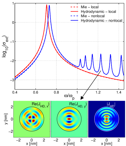
Figure 2: Simulation results for the cylindrical nanowire in Sec. 4.1. The curves show comparison of the finite element numerical solutions for the nonlocal (solid blue line) and the local (solid red line) hydrodynamic model with the corresponding analytical solutions (dashed blue line and dashed red line respectively) based on the Mie theory. The field plots show simulated hydrodynamic current $\boldsymbol{J}_{\mathrm{HD}}$ corresponding to the forth order nonlocal resonance at $\omega/\omega_{\mathrm{p}}=1.227$ (indicated by the arrow).

The finite element numerical solution for the nonlocal hydrodynamic model (solid blue line) has a prominent peak at $\omega/\omega_{\mathrm{p}}=0.731255$, which corresponds to the localized surface plasmon resonance. The subsidiary peaks beyond the bulk plasma frequency (e.g. at $\omega/\omega_{\mathrm{p}}=1.03002$, $1.07888$, $1.14547$, $1.22707$, $\cdots$ etc.) are due to the nonlocal hydrodynamic current. Consistent with the observations in Ref. [2], these peaks are present beyond the bulk plasma frequency. The positions of the localized surface plasmon resonance and the nonlocal hydrodynamic Drude resonances agree well with the analytical Mie results (the blue dashed line, which is largely covered by the solid blue line). Good agreement has been also observed in case of the local Drude model simulations; where the main peak due to the surface plasmon resonance has been shifted towards lower frequency ($\omega/\omega_{\mathrm{p}}=0.706086$, which is quite close to the theoretical estimation of $\omega/\omega_{\mathrm{p}}=1/\sqrt{2}=0.70711$).

The subplots in Fig. 2 show the simulated current density $\boldsymbol{J}_{\mathrm{HD}}$ for the nonlocal hydrodynamic resonance at $\omega/\omega_{\mathrm{p}}=1.227$. Non curl-free nature of these field plots clearly show that the quasi-static approximation (as in Ref. [5]) is inaccurate.

4.2 Plasmonic V groove channel plasmon-polariton devices

Having verified the method for the test case of cylindrical nanowires, now we demonstrate the capability of the method to handle an arbitrary shaped geometry. One of such geometries which is of a great practical interest is a channel plasmon-polariton (CPP) devices with a V groove [14]. Modal and resonance properties of such devices have been investigated thoroughly. Accurate numerical simulation of the V groove geometry is challenging due to subwavelength device features and field enhancement due to plasmonic effects [15, 16]. This makes the V groove geometry an interesting candidate to check the effect of the nonlocal response.

We simulate scattering off a V groove configuration of length $l_{1}=7$ nm, width $w_{1}=1$ nm, with a symmetrically placed groove of length $l_{2}=0.7$ nm, width $w_{2}=0.7$ nm. As shown in the inset of Fig. 3, the sharp corners of the device are rounded with the corner radius of $0.1$ nm. Note that by decreasing the corner rounding radius, the response of the V groove device will slightly change quantitatively, but we have made sure that the qualitative features are not changed significantly. The material and the hydrodynamic parameters are taken as in the case of cylindrical nanowires in Sec. 4.1. Resonance modes of the this device are excited by a unit amplitude, $x$-polarized (parallel to the length of the device ) plane wave propagating in the direction of minus $y$-axis (parallel to the width of the device). As in Sec. 4.1, we again analyze the normalized extinction cross section $\sigma_{\mathrm{ext}}$ for the V groove structure, but now the normalization is done with the length of the device $l_{1}$.

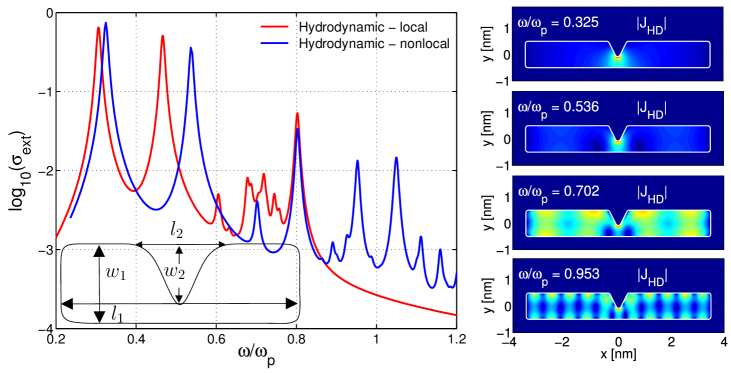
Figure 3: Left: Effect of the nonlocal material response on the resonance modes of V groove channel plasmon-polariton structures. The device parameters are as in Sec. 4.2. Right: Field distribution for the hydrodynamic current $\boldsymbol{J}_{\mathrm{HD}}$ for various nonlocal resonances of the V groove.

First we simulated the above V groove structure for the local Drude material model (the conventional model). As seen from the red curve in Fig. 3, several plasmon-polariton resonances are excited. The most interesting features are the resonances corresponding to the prominent peaks at $\omega/\omega_{\mathrm{p}}=0.306$ and $\omega/\omega_{\mathrm{p}}=0.466$, for which high electric field intensity is present in the narrow groove region [16]. On the other hand, for the resonance at $\omega/\omega_{\mathrm{p}}=0.8$, the electric field is localized at the outer vertical edges of the V groove structure, and no such particular distinction can be made for the other less prominent resonance states (e.g. the “local” resonances around $\omega/\omega_{\mathrm{p}}=0.7$).

When this V groove structure is simulated for the nonlocal Drude material model, the resonance spectrum changes significantly (the blue curve). Similar to the case of the nanowires, the both local Drude model plasmon-polariton resonances (corresponding to the high field localization in the groove) experience a shift towards high frequency ($\omega/\omega_{\mathrm{p}}=0.325$ and $\omega/\omega_{\mathrm{p}}=0.536$), but the individual extents of these shifts are different. The other local resonances are also influenced by the hydrodynamic current, resulting in high order nonlocal hydrodynamic resonances. To get a closer look at these resonances, field distributions of the hydrodynamic current are illustrated in Fig. 3. For the resonances below the the plasma frequency, for example at $\omega/\omega_{\mathrm{p}}=0.702$ and $\omega/\omega_{\mathrm{p}}=0.953$, these field plots show the oscillating hydrodynamic current; which indicates that unlike as in the case of the nanowires, for the V groove structures the plasma frequency $\omega_{\mathrm{p}}$ does not seem to separate the high order nonlocal hydrodynamic resonances from the plasmon-polariton resonances. Since the “local” resonances around $\omega/\omega_{\mathrm{p}}=0.7$ do not show any distinctive field localization properties, it is difficult to associate them with the high order nonlocal resonances. For the present simulation setting, some of these nonlocal hydrodynamic resonances are more prominent than the minor local resonances. It gives the indication with the inclusion of nonlocal effect, the resonance properties of the CPP devices change significantly.

5 Conclusions

In this work we discussed a weak formulation for the nonlocal hydrodynamic Drude model, which is simulated with Nédélec finite element method. Unlike the previously reported work [5], this approach does not use the curl-free approximation, and thus avoids spurious (i.e. model or approximation induced) resonances. The simulated results agree well with the analytical results based on the Mie theory, and the method is capable of handling arbitrary shaped scatterers. The approach discussed in this work will serve as a reference for investigating advanced hydrodynamic models, which will take into account additional physical effects.

References

- [1] C. F. Bohren, D. R. Huffman, Absorption and Scattering of light by small particles, John Wiley and Sons Ltd., 1983.
- [2] R. Ruppin, Extinction properties of thin metallic nanowires, Opt. Commun. 190 (1-6) (2001) 205–209.
- [3] S. Palomba, L. Novotny, R. E. Palmer, Blue-shifted plasmon resonance of individual size-selected gold nanoparticles, Opt. Commun. 281 (3) (2008) 480––483.
- [4] A. D. Boardman, Electromagnetic surface modes, John Wiley and Sons Ltd., 1982, Ch. Hydrodynamic theory of plasmon-polaritons on plane surfaces, pp. 1–76.
- [5] J. M. McMahon, S. K. Gray, G. C. Schatz, Calculating nonlocal optical properties of structures with arbitrary shape, Phys. Rev. B 82 (2010) 035423.
- [6] S. Raza, G. Toscano, A. P. Jauho, M. Wubs, N. A. Mortensen, Unusual resonances in nanoplasmonic structures due to nonlocal response, Phys. Rev. B 84 (2011) 121412.
- [7] G. Toscano, S. Raza, A.-P. Jauho, N. A. Mortensen, M. Wubs, Modified field enhancement and extinction by plasmonic nanowire dimers due to nonlocal response, Opt. Express 20 (4) (2012) 4176–4188.
- [8] A. Bondeson, T. Rylander, P. Ingelström, Computational Electromagnetics, Vol. 51 of Texts in Applied Mathematics, Springer, 2005.
- [9] J. C. Nédélec, A new family of mixed finite elements in , Numer. Math. 50 (1) (1986) 57–81.
- [10] P. Monk, Finite Element Methods for Maxwell’s equations, Oxford Science Publications, 2003.
- [11] L. Zschiedrich, Transparent boundary conditions for Maxwell’s equations: Numerical concepts beyond the PML method, Ph.D. thesis, Frei Universität Berlin (2009).
- [12] J. Pomplun, S. Burger, L. Zschiedrich, F. Schmidt, Adaptive finite element method for simulation of optical nano structures, phys. stat. sol. (b) 244 (10) (2007) 3419–3434.
- [13] G. Toscano, M. Wubs, S. Xiao, M. Yan, Z. F. Öztürk, A.-P. Jauho, N. A. Mortensen, Plasmonic nanostructures: local versus nonlocal response, Proc. SPIE 7757 (1) (2010) 77571T–1–7.
- [14] S. I. Bozhevolnyi, V. S. Volkov, E. Devaux, J.-Y. Laluet, T. W. Ebbesen, Channel plasmon subwavelength waveguide components including interferometers and ring resonators, Nature 440 (7083) (2006) 508–511.
- [15] E. Moreno, F. J. Garcia-Vidal, S. G. Rodrigo, L. Martin-Moreno, S. I. Bozhevolnyi, Channel plasmon-polaritons: modal shape, dispersion, and losses, Opt. Lett. 31 (23) (2006) 3447–3449.
- [16] C. Hafner, X. Cui, A. Bertolace, R. Vahldieck, Frequency-domain simulations of optical antenna structures, Proc. SPIE 66170 (2007) 66170E–1–12.