On the Transitional Disk Class: Linking Observations of T Tauri Stars & Physical Disk Models

Abstract

Two decades ago “transitional disks” described spectral energy distributions (SEDs) of T Tauri stars with small near-IR excesses, but significant mid- and far-IR excesses. Many inferred this indicated dust-free holes in disks, possibly cleared by planets. Recently, this term has been applied disparately to objects whose Spitzer SEDs diverge from the expectations for a typical full disk. Here we use irradiated accretion disk models to fit the SEDs of 15 such disks in NGC 2068 and IC 348. One group has a “dip” in infrared emission while the others’ continuum emission decreases steadily at all wavelengths. We find that the former have an inner disk hole or gap at intermediate radii in the disk and we call these objects “transitional” and “pre-transitional” disks, respectively. For the latter group, we can fit these SEDs with full disk models and find that millimeter data are necessary to break the degeneracy between dust settling and disk mass. We suggest the term “transitional” only be applied to objects that display evidence for a radical change in the disk’s radial structure. Using this definition, we find that transitional and pre-transitional disks tend to have lower mass accretion rates than full disks and that transitional disks have lower accretion rates than pre-transitional disks. These reduced accretion rates onto the star could be linked to forming planets. Future observations of transitional and pre-transitional disks will allow us to better quantify the signatures of planet formation in young disks.

1. Introduction

Disks around T Tauri stars (TTS) are thought to be the sites of planet formation. However, many questions exist concerning how the gas and dust in the disk evolve into a planetary system and observations of TTS may provide clues. There are some objects in particular that have gained increasing attention in this regard. Over two decades ago, Strom et al. (1989) detected “possible evidence of changes in disk structure with time” as evidenced by “small near-IR excesses, but significant mid- and far-IR excesses” indicating “inner holes” in disks. Those authors proposed that these objects were “in transition from massive, optically thick structures that extend inward to the stellar surface, to low-mass, tenuous, perhaps post-planet-building structures.”

Usage of the term “transitional disk” gained substantial momentum in the literature after it was used by Calvet et al. (2005b) to describe disks with inner holes using data from the Spitzer Space Telescope’s (Werner et al., 2004) Infrared Spectrograph (IRS; Houck et al., 2004). Before Spitzer, the spectral energy distributions (SEDs) used to identify disks with inner holes were based solely on near-infrared (NIR) ground-based photometry and IRAS mid-IR (MIR) photometry (Strom et al., 1989; Skrutskie et al., 1990). Spitzer allowed the opportunity to study these objects in greater detail. The unprecedented resolution and simultaneous wavelength coverage ($\sim$5 and 38 $\mu$m) of Spitzer IRS uncovered new details regarding these disks (D’Alessio et al., 2005; Calvet et al., 2005b; Furlan et al., 2006). Some SEDs had nearly photospheric NIR (1–5 $\mu$m) and MIR (5–20 $\mu$m) emission, coupled with substantial emission above the stellar photosphere at wavelengths beyond $\sim$20 $\mu$m. Others had significant NIR excesses relative to their stellar photospheres, but still exhibited MIR dips and substantial excesses beyond $\sim$20 $\mu$m.

Detailed modeling of many of the above-mentioned SEDs has been performed. SEDs of disks with little or no NIR and MIR emission have been fit with models of inwardly truncated optically thick disks (Calvet et al., 2002, 2005b; Espaillat et al., 2007b, 2008b). The inner edge or “wall” of the outer disk is frontally illuminated by the star, dominating most of the emission seen in the IRS spectrum. In this paper, we refer to these objects with holes in their dust distribution as transitional disks (TD). Some of the holes in TD are relatively dust-free (e.g. DM Tau; Calvet et al., 2005b; Espaillat et al., 2010) while SED model fitting indicates that others with strong 10$\mu$m silicate emission have a small amount of optically thin dust in their disk holes to explain this feature (e.g. GM Aur; Calvet et al., 2005b; Espaillat et al., 2010). For SEDs with substantial NIR emission accompanied by a MIR dip, we can fit the observed SED with an optically thick inner disk separated by an optically thin gap from an optically thick outer disk (Espaillat et al., 2007a). Here we call these pre-transitional disks (PTD). Like the TD, we see evidence for relatively dust-free gaps (e.g. UX Tau A; Espaillat et al., 2007a, 2010) as well as gaps with some small, optically thin dust to explain strong 10$\mu$m silicate emission features (e.g. LkCa 15; Espaillat et al., 2007a, 2010). For many TDs and PTDs, the truncation of the outer disk has been confirmed with sub-millimeter and millimeter interferometric imaging (e.g. DM Tau, GM Aur, UX Tau A, LkCa 15; Hughes et al., 2007, 2009; Andrews et al., 2009, 2010, 2011) as well as NIR imaging (i.e. LkCa 15; Thalmann et al., 2010). In a few cases, the optically thick inner disk of PTD has been confirmed using the “veiling” of near-infrared spectra (Espaillat et al., 2008a, 2010) and near-infrared interferometry has confirmed that the inner disk is small (Pott et al., 2010; Olofsson et al., 2011).

The distinct SEDs of TD and PTD most likely signify that these objects are being caught in an important phase in disk evolution. Many researchers have posited that these disks are forming planets on the basis that cleared dust regions are predicted by planet formation models (e.g. Paardekooper & Mellema, 2004; Zhu et al., 2011; Dodson-Robinson & Salyk, 2011). Recently, a potential protoplanet has been reported in the pre-transitional disk around LkCa 15 (Kraus et al., 2011) as well as around T Cha (Huélamo et al., 2011). Stellar companions can also clear the inner disk (Artymowicz & Lubow, 1994) but many stars harboring transitional disks are single stars (Kraus et al., 2011). Even in cases where stellar-mass companions have not been ruled out, the large holes and gaps observed are most likely evidence of dynamical clearing. Photoevaporation cannot explain disks with large cavities and high mass accretion rates (Owen et al., 2011) and dust evolution alone can not explain the sharp decreases in surface density seen in the SED and interferometric visibilities.

Given the potential link between disks with gaps and holes and planet formation, interest in transitional disks has grown. Some studies have focused on further understanding the behavior of the currently known members in this class of objects and have discovered IR variability (Muzerolle et al., 2010; Espaillat et al., 2011, E11). Other studies have taken a broader approach, working towards expanding the known number of disks undergoing clearing (e.g. Lada et al., 2006; Hernández et al., 2007; Cieza et al., 2010; Muzerolle et al., 2010; Luhman et al., 2010; Merín et al., 2010; Currie & Sicilia-Aguilar, 2011). As the literature on Spitzer observations of TTS expands, so does the terminology applied to disks around TTS. These disks are referred to as primordial, full, transitional, pre-transitional, kink, cold, anemic, homologously depleted, classical transitional, weak excess, warm excess, and evolved. However, these terms are not applied consistently. The issue is highlighted with the discrepancies in the reported fractions of transitional disks and disk clearing timescales (Merín et al., 2010; Luhman et al., 2010; Muzerolle et al., 2010; Currie & Sicilia-Aguilar, 2011; Hernández et al., 2010). In many cases, the data is the same; the differences arise from nomenclature.

If the goal is to better understand disk evolution, it is important to look past the nomenclature and decipher the underlying disk structure we can infer from the observations, while paying special attention to the limitations of both the observations and the tools we use to interpret them, namely disk models. To this end, we chose a sample for our study which incorporated objects whose SEDs are similar to those that have been referred to as “transitional” in the literature. We focus on 15 disks in NGC 2068 and IC 348 with Spitzer IRS spectra. NGC 2068 and IC 348 are older ($\sim$2 Myr and $\sim$3 Myr, respectively; Flaherty & Muzerolle, 2008; Luhman et al., 2003) and more clustered star-forming regions with higher extinction than Taurus, where most detailed studies of transitional disks have focused. According to our definitions stated above, our sample contains five TD, five PTD, and five objects with decreasing emission at all IR wavelengths (i.e. negative MIR slopes) which we classify as full disks. Out of the objects reported by Muzerolle et al. (2010), this includes 5 of the 15 transitional and pre-transitional disks in IC 348 and 4 of the 6 transitional and pre-transitional disks in NGC 2068. One of the objects classified as a full disk in that work is classified as a PTD here.

In Section 2, we present optical photometry and spectroscopy, infrared spectra, and millimeter flux densities that we used to compile SEDs for our objects, derive stellar properties, and measure mass accretion rates. In Section 3, we fit the SEDs of our objects with irradiated accretion disk models and in Section 4 we discuss the limitations of the models and the observations, disk semantics, and the mass accretion rates of transitional and pre-transitional disks.

2. Observations & Data Reduction

Before conducting modeling, we first compiled SEDs and mass accretion rates for the targets in our sample (Table 1). To supplement the existing information in the literature, we collected optical photometry for all of our IC 348 objects, optical spectra for three of the IC 348 targets and all of our NGC 2068 targets, and millimeter flux densities for two of our IC 348 targets. We also present infrared spectra for all the targets in this paper. Below we discuss the details of the observations and data reduction.

2.1. Optical Photometry

During November 19–23, 2011 we used the 4K CCD imager on the 1.3-m McGraw-Hill telescope of the MDM Observatory to obtain UVRI photometry of the IC348 stellar cluster. The FOV of the instrument is 21^′$\times$21^′ (0.315^′′ per unbinned pixel). For these observations, we used 2$\times$2 binning (0.62^′′ per pixel). The flat-field, overscan, and astrometric calibration were performed using an IDL program written by Jason Eastman specifically designed for the 4K CCD imager. Since large electronic structures are not stable enough to be reliably subtracted, we did not apply corrections using two dimensional biases. The photometric calibration of all images was carried out using the standard procedure and the daophot and photcal packages in IRAF, with standard stars selected from Landolt (1992). Photometry is presented in Table 2.

2.2. Optical Spectroscopy

In order to obtain mass accretion rate estimates (Section 3.1.1 and Figure 1), we collected MIKE double-echelle spectrograph (Bernstein et al., 2003) data on the 6.5m Magellan Clay telescope for all of our targets in NGC 2068 (FM 177, FM 281, FM 515, FM 581, and FM 618) and some of our objects in IC 348 (LRLL 21, LRLL 67, and LRLL 72). The observations for the NGC 2068 and IC 348 objects were taken on February 10-11, 2007 and January 19, 2009, respectively. We used a slit size of 0.7^′′$\times$5.0^′′ and 2$\times$2 pixel on-chip binning with exposure times of 800-1200s. Data were reduced using the MIKE data reduction pipeline.

2.3. Infrared Spectroscopy

Here we present Spitzer IRS spectra for each of our targets. Spectra for NGC 2068 and IC 348 were obtained in Program 58 (PI: Rieke) and Program 2 (PI: Houck), respectively. All of the observations were performed in staring mode using the IRS low-resolution modules, Short-Low (SL) and Long-Low (LL), which span wavelengths from 5–14 $\mu$m and 14-38 $\mu$m, respectively, with a resolution $\lambda/\delta\lambda\sim$90.

Details on the observational techniques and general data reduction steps can be found in Furlan et al. (2006) and Watson et al. (2009). We provide a brief summary. Each object was observed twice along the slit, at a third of the slit length from the top and bottom edges of the slit. Basic calibrated data (BCD) with pipeline version S18.7 were obtained from the Spitzer Science Center. With the BCDs, we extracted and calibrated the spectra using the SMART package (Higdon et al., 2004). Bad and rogue pixels were corrected by interpolating from neighboring pixels.

Most of the data were sky subtracted using optimal extraction (Lebouteiller et al., 2010). The exceptions were LRLL 37, LRLL 55, and LRLL 68. In LRLL 37, there was an artificial structure in the 5–8 $\mu$m region which was removed by performing off-nod sky subtraction. A similar structure was seen in LRLL 55 and LRLL 68, but due to the high background in the area, optimal extraction was necessary for the LL order. Therefore, the final spectra for LRLL 55 and LRLL 68 are a combination of the off-nod sky-subtracted SL spectra and the optimally extracted LL spectra.

To flux calibrate the observations we used a spectrum of $\alpha$ Lac (A1 V). We performed a nod-by-nod division of the target spectra and the $\alpha$ Lac spectrum and then multiplied the result by a template spectrum (Cohen et al., 2003). The final spectrum was produced by averaging the calibrated spectra from the two nods. Our spectrophotometric accuracy is 2–5$\%$ estimated from half the difference between the nodded observations, which is confirmed by comparison with IRAC and MIPS photometry. We note that there are artifacts in the spectra of LRLL 68 and LRLL 133 beyond $\sim$30 $\mu$m. For clarity, we manually trim the spectra to exclude these regions. The final spectra used in this study are shown in Figures 2, 3, and 4.

2.4. Millimeter Flux Densities

We observed LRLL 21, LRLL 31, LRLL 67, LRLL 68, and LRLL 72 in IC 348 with the Submillimeter Array (SMA) on November 12, 2008. We used the Compact Configuration with six of the 6 meter diameter antennas at 345 GHz (860 $\mu$m) with a full correlator bandwidth of 2 GHz. Calibration of the visibility phases and amplitudes was achieved with observations of the quasars 3C 111 and 3C 84, typically at intervals of 20 minutes. Observations of Uranus provided the absolute scale for the flux density calibration. The data were calibrated using the MIR software package. We detected LRLL 31 and LRLL 67 with flux densities of 0.062$\pm$0.006 Jy and 0.025$\pm$0.011 Jy, respectively. We did not detect LRLL 21, LRLL 68, or LRLL 72 and measure a 3${\sigma}$ upper limit of 0.015 Jy for these objects.

3. Analysis

Here we model the SEDs of the targets in our sample. First we collect the stellar properties of our objects, either by adopting literature values or deriving our own in Section 3.1. These stellar properties are important input parameters for our physically motivated models which we discuss in Section 3.2. In Section 3.3 we discuss the results of our SED model fitting, as well as the degeneracies that exist given that we lack millimeter observations for many of our targets.

3.1. Stellar Properties

Stellar parameters are listed in Table 3. M_∗ was derived from the HR diagram and the Siess et al. (2000) evolutionary tracks using T_∗ and L_∗. Stellar temperatures are from Kenyon & Hartmann (1995), based upon the spectral types adopted for the targets in NGC  2068 and IC 348 (Flaherty & Muzerolle, 2008; Luhman et al., 2003, respectively). Luminosities are calculated with dereddened J-band photometry following Kenyon & Hartmann (1995) assuming a distance of 400 pc for NGC 2068 (Flaherty & Muzerolle, 2008) and 315 pc for IC 348 (Luhman et al., 2003). R_∗ is calculated using the derived luminosity and adopted temperature. The derivation of the mass accretion rates and accretion luminosities are discussed in Section 3.1.1.

All photometry for our NGC 2068 objects is taken from Flaherty & Muzerolle (2008). This includes BVRI, 2MASS JHK, IRAC, and MIPS data. We note that Flaherty & Muzerolle (2008) present photometry from the SDSS survey, which we convert to Johnson-Cousins BVRI following Jordi et al. (2006). IRAC and MIPS photometry for IC 348 comes from Lada et al. (2006) and 2MASS JHK data is from Skrutskie et al. (2006). UBVRI photometry for our IC 348 targets comes mainly from this work, but is supplemented by values in the literature. All UBVRI photometry for LRLL 31, LRLL 55, LRLL 67, LRLL 68, LRLL 72, and LRLL 133 are solely from this work. UVR data for LRLL 21 and LRLL 37 are from this work, but we use I-band magnitudes from Luhman et al. (2003) for both and a B-band magnitude for LRLL 21 from Herbig (1998). We use R and I data from Herbig (1998) for LRLL 2. BVRI data for LRLL 6 is also from Herbig (1998). All L-band magnitudes are from Haisch et al. (2001).

Extinctions were measured by comparing V-R, V-I, R-I, and I-J colors to photospheric colors from Kenyon & Hartmann (1995). We used the Mathis (1990) extinction law for objects with A_V$<$ 3. For A_V$\geq$ 3, we use the McClure (2009) extinction law. We adopt R_V=5 which is more appropriate for the denser regions studied here (Mathis, 1990). In most cases, extinctions based on I-J colors gave the best fit. Since we have no I-band data for FM 581 we adopt an extinction based on V-R; LRLL 2 and LRLL 6 have no VRI photometry in the literature and so we adopt the extinction measured by Luhman et al. (2003). All extinctions used in this work are listed in Table 3. We note that most of our extinctions are similar to those in the literature (Luhman et al., 2003; Flaherty & Muzerolle, 2008). In cases where we found differences, we chose to rely on our measurements since they are based on I-J colors which have recently been shown to be the least affected by excess emission at shorter wavelengths (Fischer et al., 2011, McClure et al., in preparation). For early-type stars, the peak of the stellar emission would be at shorter wavelengths. However, the early-type star in our sample (LRLL 2) has bad photometry so we do not explore this point further.

3.1.1 Accretion Rates

During the classical TTS phase of stellar evolution, young objects accrete material from the disk onto the star via magnetospheric accretion (Uchida & Shibata, 1984). The infalling gas impacts the stellar surface at approximately the free fall velocity creating a shock which heats the gas to $\sim$ 1 MK (Calvet & Gullbring, 1998). The shock emission is reprocessed in the accretion column and the observed spectrum peaks in the ultraviolet (Calvet & Gullbring, 1998). The best estimate of the accretion rate is found by measuring the total luminosity emitted in the accretion shock, i.e. the accretion luminosity. While ultraviolet emission is difficult to observe from ground-based observatories, there are many tracers of the accretion luminosity at longer wavelengths (see Rigliaco et al. (2011) for a comprehensive list). A few of those tracers include excess emission observed in U-band photometry, emission in the NIR Ca II triplet lines, and the H$\alpha$ line profile.

Second to the ultraviolet excess, U-band excesses are the best measure of the flux produced in the shock and have been shown to correlate with the total shock excess (Calvet & Gullbring, 1998). However, at low $\dot{M}$ emission at $U$ may be dominated by chromospheric emission (Houdebine et al., 1996; Franchini et al., 1998); this chromospheric excess can confuse determinations of the accretion rate (Ingleby et al., 2011). While possible from the ground, U-band observations are still difficult to obtain, especially when extinction towards the source is relatively high as in the case of our sample, all with $A_{V}>1$. Observations of the Ca II near-infrared triplet are easily obtained from the ground, even for high $A_{V}$ sources, and the flux in the 8542 Å line also correlates with the accretion luminosity (Muzerolle et al., 1998). Ca II is observed in emission in accreting sources but is unreliable at low accretion rates, when the chromospheric emission rivals that from accretion in strength (Yang et al., 2007; Batalha & Basri, 1993; Ingleby & et al., 2011). H$\alpha$ is commonly used as a tracer of accretion, both by measuring the equivalent width and the velocity width of the line in the wings (White & Basri, 2003; Barrado y Navascués & Martín, 2003; Natta et al., 2004). Models of magnetospheric accretion have reproduced the observed velocities in H$\alpha$, tracing material traveling at several hundred km s^-1 near the accretion shock (Lima et al., 2010; Muzerolle et al., 2003).

The mass accretion rates adopted for our sample are listed in Table 3. We used U-band photometry from this work and the relation in Gullbring et al. (1998) to measure mass accretion rates for LRLL 37 and LRLL 68 and an upper limit for LRLL 133. For FM 177, FM 281, FM 515, FM 581, FM 618, LRLL 21, LRLL 67, and LRLL 72, we used high resolution echelle spectra obtained with MIKE to measure the width of the H$\alpha$ line in the wings (at 10% of the maximum flux; Figure 1). We then compared this to the relation between line width and $\dot{M}$ in Natta et al. (2004) to obtain mass accretion rate estimates for these eight sources. While our MIKE spectra covered both H$\alpha$ and the Ca II triplet, H$\alpha$ provided a more accurate estimate of $\dot{M}$ due to confusion with chromospheric Ca II emission at the levels of accretion found in these sources. Given the chromospheric appearance of the H$\alpha$ profile of LRLL 72, its mass accretion rate should be taken as an upper limit. For LRLL 31 we adopted a mass accretion rate from the literature. We do not have mass accretion rate measurements for LRLL  2 or LRLL 6.

For NGC 2068, we compared our derived accretion rates to those in Flaherty & Muzerolle (2008) who calculated the amount of excess continuum emission necessary to produce the observed veiling of the photospheric lines. Within a factor of 2–3, the normal error in $\dot{M}$ estimations, both calculations of the accretion rate agree, with a few exceptions. When comparing the H$\alpha$ line widths at 10% we find that our MIKE line profile of FM 281 is $\sim 180\;\rm{km\;s^{-1}}$ narrower than when observed by Flaherty & Muzerolle (2008). In addition, our observation of FM 177 is consistent with an accreting source, while when observed by Flaherty & Muzerolle (2008) its H$\alpha$ profile was consistent with that of chromospheric emission. Variability is known to occur in T Tauri stars so the decrease in H$\alpha$ and $\dot{M}$ are not unexpected (Cody & Hillenbrand, 2010). For these objects we chose to adopt the accretion rate obtained from our MIKE observations. The biggest uncertainty in calculating accretion rates using veiling is the choice of bolometric correction, which can vary in value by a factor of 10 depending on which analysis is used (White & Hillenbrand, 2004) and the spectrum of the excess emission which veils the photospheric lines can be complicated (Fischer et al., 2011).

3.2. Disk Model

We try to reproduce the SEDs presented in Figures 2, 3, & 4 using the irradiated accretion disk models of D’Alessio et al. (1998, 1999, 2001, 2005, 2006). We point the reader to those papers for details of the model and to Espaillat et al. (2010) for a summary of how we apply the model to the SEDs of transitional and pre-transitional disks. Here we provide a brief review of the salient points of the above works.

When we refer to a “full disk model” we mean a disk model composed of an irradiated accretion disk and a frontally illuminated wall at the inner edge of the disk which is located at the dust sublimation radius. The inner wall dominates the emission in the NIR, the wall and disk both contribute to the MIR emission, and the disk dominates the emission at longer wavelengths. Compared to a full disk model, a pre-transitional disk model has a gap within the disk. In this case, we include a frontally illuminated wall at the dust sublimation radius and another wall at the gap’s outer edge. For this outer wall we include the shadow cast by the inner wall (Espaillat et al., 2010). We do not include an inner irradiated accretion disk behind the inner wall since previous work has shown that the inner wall dominates the emission at these shorter wavelengths (Espaillat et al., 2010). Behind the outer wall we include an irradiated accretion disk in cases where we have millimeter data, which is necessary to constrain the outer disk. The inner wall dominates the NIR emission while the outer wall dominates the emission from $\sim$20–30 $\mu$m. The outer disk dominates the emission beyond $\sim$40 $\mu$m. A transitional disk model is very similar to that of a pre-transitional disk model except that we do not include an inner wall at the dust sublimation radius. In some instances, we include a small amount of optically thin dust in the inner hole or gap in transitional and pre-transitional disks to reproduce the 10 $\mu$m silicate emission feature. We calculate the emission from this optically thin dust region following Calvet et al. (2002).

3.2.1 Disk Properties

Table 4 lists the model-derived properties of our sample. The heights of the inner and outer walls (z_wall) and the maximum grain sizes (a_max) are adjusted to fit the SED. $T_{wall}$ is the temperature at the surface of the optically thin wall atmosphere. The temperature of the inner wall of full disks and pre-transitional disks (T${}_{wall}^{i}$) is held fixed at 1400 K (except for FM 515, see Section 3.3) which is the typical temperature of dust at the sublimation radius (Muzerolle et al., 2003). The temperature of the outer wall (T${}_{wall}^{o}$) in transitional and pre-transitional disks is varied to fit the SED, particularly the IRS spectrum. The radius of the wall ($R_{wall}$) is derived using the best fitting $T_{wall}$ following Equation 2 in Espaillat et al. (2010).

Previously, we have seen that in transitional and pre-transitional disks, the IRS spectrum is dominated by the outer wall while the outer disk dominates the millimeter emission (E11). Since the majority of the emission seen by IRS is from the outer wall, the IRS spectrum is a good constraint of the hole$/$gap size and in most cases SED-derived hole$/$gap sizes are in reasonable agreement with those obtained with millimeter imaging (Andrews et al., 2011). For objects in this work with no millimeter data, we do not include an outer disk given that its contribution to the IRS SED is expected to be small. We did include an outer disk for the two objects in the sample for which we have millimeter data: the transitional disk LRLL 67 and the pre-transitional disk LRLL 31. We also included an outer disk when modeling each of our full disk targets since additional emission from an outer disk is necessary to reproduce the observed MIR emission. The parameters of the outer disk which are varied to fit the SED are the viscosity parameter ($\alpha$) and the settling parameter ($\epsilon$; see Section 3.2.2). One can interpret varying $\alpha$ as fitting for the disk mass since M${}_{disk}\propto{\hbox{$\dot{M}$}}/{\alpha}$ (see Equation 38 in D’Alessio et al., 1998). We note that the mass accretion rate onto the star does not necessarily reflect the mass transport across the outer disk, especially in the case of TD and PTD where the mass accretion rate onto the star is likely an underestimate of the mass transport across the outer disk (see Section 4.4). We also do not expect that the mass accretion rate is constant throughout the disk. However, for simplicity, here we assume that the mass accretion rate measured onto the star is representative of the disk’s accretion rate.

We will discuss how the lack of millimeter constraints leads to degeneracies in our outer disk model fitting in Section 3.3. There we also discuss the effect the adopted disk inclination and outer radius have on the simulated SED. We assume that the inclination of the disk is 60^∘ for all of our objects and that they have an outer disk radius of 300 AU (except FM 581, see Section 3.3).

3.2.2 Dust Properties

The opacity of the disk, and hence the temperature structure and resulting emission, is controlled by dust. The dust opacity depends on the composition of the dust assumed. It also depends on changes in the dust due to grain growth and settling. Grains grow through collisional coagulation and settle to the disk midplane due to gravity. Since in this work we include models of several full disks, here we review the effect that the dust properties have on the disk structure in more detail following D’Alessio et al. (2006).

Dust Settling. The settling of dust has important, and often overlooked, effects on the disk’s density–temperature distribution and emission. When there is some degree of settling, the dust-to-gas mass ratio of grains in the disk atmosphere decreases with respect to the standard value (i.e. the diffuse interstellar medium). This has several effects: (1) it decreases the opacity of the upper layers; this allows the impinging external radiation to penetrate deeper into the disk, decreasing the height of the irradiation surface and making it geometrically flatter (see Figure 3 in D’Alessio et al., 2006), which in turn decreases the fraction of the irradiation flux intercepted by this surface, decreasing the continuum flux emerging from the disk, (2) since most of the external radiation is deposited at the irradiation surface, lowering it changes the temperature-density structure of the atmospheric layers, where the temperature inversion occurs (also called the super-heated layers), modifying their contribution to the SED, and finally, (3) it changes the emissivity of the disk interior; in this region the dust-to-gas mass ratio of the grains increases given that the grains removed by depletion from the upper layers are now located deeper in the disk.

Some of the above-mentioned effects can be accounted for by arbitrarily changing the disk surface height as a function of radius (e.g. Miyake & Nakagawa, 1995; Currie & Sicilia-Aguilar, 2011; Sicilia-Aguilar et al., 2011), and this will probably give a reasonable estimate of the continuum SED of the disk. However, the contribution of the upper layers to the SED or the role of the deeper layers in millimeter images and emergent flux, would not be consistent for this simple approach to settling. On the other hand, taking into account the detailed physics of settling (e.g. Weidenschilling et al., 1997; Dullemond & Dominik, 2004) is complex and simulations show that disks should be completely settled within $\sim$10⁶ years, in contradiction with observations, reflecting that we are missing some processes that can keep some small grains in the upper layers for longer timescales (e.g. turbulence; Dullemond & Dominik, 2005; Birnstiel et al., 2011).

In our SED modeling we have adopted a different approach following D’Alessio et al. (2006) by parameterizing settling as a depletion of dust in the upper layers, with a corresponding increment of the dust-to-gas mass ratio near the midplane. The maximum grain sizes in the disk atmosphere and interior are allowed to change, reflecting the possibility of grain growth. We can also vary the height in the disk that separates the atmosphere from the interior as well as the degree of settling. The amount of settling is parameterized by $\epsilon=\zeta_{atm}/\zeta_{std}$, (i.e., the dust-to-gas mass ratio of the disk atmosphere divided by the standard value). The main point of this approach is that the same grains that determine the height and shape of the irradiation surface and the amount of intercepted external flux, are the ones that are emitting in the mid-IR silicate bands, and their emissivity and temperature distribution are consistent with their properties. Also, the grains near the midplane which are responsible for the mm emergent intensity have a dust-to-gas mass ratio related to the properties of the atmospheric grains. The advantage of such an approach is that, in principle, observations can be used to constrain the grains’ composition, size and spatial distribution, and this can be related to models of the detailed dust evolution in disks. However, to really fulfill this goal, we need observations that cover a wide range of wavelengths with high resolution. Given our present observations, we have chosen to adopt a radially constant $\epsilon$ and to assume that the interior grains are concentrated very close to the midplane (at z $\lesssim$ 0.1 H). These assumptions will not affect the mid-IR SED (D’Alessio et al., 2006, Qi et al. 2011) and we avoid introducing new sets of free parameters to the problem, retaining the important physical properties of settling.

Dust Grain Growth. In this work we also change the maximum grain size in the disk. The models assume spherical grains with a distribution of $a^{-p}$ where $a$ is the grain radius between a_min and a_max and p is 3.5 (Mathis et al., 1977). A mixture with a smaller a_max has a larger opacity at shorter wavelengths than a mixture with a larger a_max. Since the height of the disk surface, $z_{s}$, is defined by the region where $\tau_{s}\sim 1$ small grains will reach this limit higher in the disk relative to big grains. Therefore, disks with a small a_max are more flared than disks with a large a_max for the same dust-to-gas mass ratio. One difference between increasing the settling and increasing the grain size is that with settling, small grains remain in the upper disk layers and so we still see silicate emission while with grain growth in the disk atmosphere, the silicate emission disappears since larger grains do not have this feature in their opacity. In the walls and the outer disk, $a_{min}$ is held fixed at 0.005 $\mu$m while $a_{max}$ is varied between 0.25 $\mu$m and 10 $\mu$m to achieve the best fit to the silicate emission features. In the outer disk, there are two dust grain size distributions as mentioned above. In the disk interior the maximum grain size is 1 mm (D’Alessio et al., 2006). The maximum grain size of the disk atmosphere is adjusted as noted earlier.

Dust Composition. The composition of dust used in the disk model impacts the resulting SED and derived disk properties (see Espaillat et al. (2010) for a discussion). We follow E11 and perform a detailed dust composition fit for the silicates seen in the IRS spectra including olivines, pyroxenes, forsterite, enstatite, and silica. We list the derived silicate mass fractions in Tables 6 and 7 of the Appendix. In addition to silicates, we also included organics, troilite, and water ice following Espaillat et al. (2010) and E11. We note that only silicates exist at the high temperatures at which the inner wall is located. In transitional and pre-transitional objects where we include optically thin dust within the hole, the silicate dust composition and abundances are listed in Tables 8 and 9 of the Appendix, respectively.

3.3. SED Modeling

In this work we present the first detailed modeling of disks with IRS spectra in NGC 2068 and IC 348. We find that all the objects are reasonably reproduced with transitional, pre-transitional, or full disk models. It is not the goal of this paper to find a unique fit to the SED. To arrive at a unique fit, one would ideally have a finely sampled, multi-wavelength SED as well as spatially resolved data at multiple wavelengths. Finely sampled data on the time domain would also be necessary since the emission of TTS is known to be variable (e.g. Espaillat et al., 2011). Given that this situation is not currently achievable, here we focus on finding a fit that is consistent with the observations presented in this work. Our assumptions of the disk structure are an oversimplification. Recent hydrodynamical simulations show that the inner regions of transitional and pre-transitional disks should be complex (Zhu et al., 2011; Dodson-Robinson & Salyk, 2011). However, in the absence of data capable of confirming these simulations, we proceed with our simple model. We discuss additional assumptions and how they play into the degeneracies of our modeling in Section 4.2. We present details of the derived dust composition in the Appendix.

3.3.1 Results

We find a large range of hole and gap sizes for our transitional and pre-transitional disks. Our TD have holes spanning 4 to 49 AU (Figure 5, Table 4). Our pre-transitional disk targets have gaps ranging from 5–45 AU (Table 4 and Figures 5, 6, and 7). The three objects easily identified by dips in the SED (FM 515, FM 618, LRLL 31) have gap sizes of 11-45 AU. We note that here we classify LRLL 21 as a PTD even though its NIR emission is weaker than the other PTD in our sample and it resembles the emission expected from a TD. Flaherty et al. (2012) find that LRLL 21 has significant NIR emission in more recent IRS observations, pointing to strong intrinsic variability in the inner disk linked to changes in the inner wall (Espaillat et al., 2011). Therefore, here we classify LRLL 21 as a PTD. Another PTD in our sample that is not obvious based on its SED alone is LRLL 37 which has the smallest gap size in our sample (5 AU; Figure 6). It is not possible to fit the IRS data of LRLL 37 with a full disk model, even within the uncertainties of the observations. In particular, we could not fit the strong 10 $\mu$m silicate emission with our full disk model. This could be a sign that LRLL 37 is a pre-transitional disk with a small gap that contains some small optically thin dust, reminiscent of RY Tau (E11) and we will return to this point in Section 4.1. We only have millimeter fluxes for two objects in our sample, LRLL 31 and LRLL 67. For these disks we derive a disk mass of 0.06 M_⊙ for each (Figure 7). The best fitting $\epsilon$ and $\alpha$ for LRLL 31 are 0.001 and 0.005, respectively. For LRLL 67, $\epsilon$=0.001 and $\alpha$=4$\times$10^-5.

Most of the transitional and pre-transitional disks have small optically thin dust within the inner 1 AU of the hole or gap. The exceptions are the transitional disk LRLL 72, where we find the 10 $\mu$m silicate emission can be produced by the optically thin atmosphere of the outer wall, and the pre-transitional disk LRLL 31, where the 10 $\mu$m silicate emission comes from the inner wall’s atmosphere and optically thin dust within the gap is not necessary to fit the observations. The mass of dust and sizes of the grains in this region are given in the Appendix.

For FM 581, LRLL 2, LRLL 6, LRLL 55, and LRLL 68 we can fit the SED reasonably well using full disk models (Figure 8). Unlike LRLL 31 and LRLL 67 above, we do not have millimeter detections for FM 581, LRLL 2, LRLL 6, LRLL 55, and LRLL 68 and so we cannot constrain the mass of the disk. Therefore, the models presented here are more uncertain, but we show them to illustrate that a disk model with dust settling and no holes or gaps in the disk can reproduce the observed SEDs. We do have an upper limit for the millimeter flux of LRLL 68 and we use this object as an example to discuss the degeneracies inherent in the modeling presented, mainly due to lack of millimeter detections, in Section 3.3.2. To briefly summarize, disk models with the same ${\epsilon}$-to-$\alpha$ ratio will produce very similar emission in the IR but substantially different emission in the millimeter. Therefore, millimeter data is crucial to disentangle this degeneracy and the disk parameters in this work should only be taken as indicative of a model that can reproduce the observed SEDs.

With the above degeneracies in mind, we limited our parameter search and set ${\epsilon}$=0.001, changing only $\alpha$ until we achieved a good fit to the SED. We could have also set $\alpha$ to a certain value and fit for $\epsilon$ instead, however, as mentioned above and as discussed in Section 3.3.2, ${\epsilon}$$/$$\alpha$ is the most relevant result. For LRLL 2, LRLL 55, and LRLL 68 we find $\alpha$=0.06, 0.004, 0.006, respectively. For LRLL 6 using an ${\epsilon}$ of 0.001 required $\alpha$$>$0.1 which would lead to a viscous timescale shorter than the lifetime of the disk (Hartmann et al., 1998), so instead we set ${\epsilon}$= 0.0001; the best-fitting $\alpha$ in this case was 0.1. To fit the very steep downward slope of FM 581, we needed to significantly truncate the outer disk radius, down to 0.6 AU. We fit FM 581 with $\epsilon$=0.001 and $\alpha$=0.00006.

3.3.2 Model Degeneracies and Millimeter Constraints

Here we explore the degeneracies introduced into the modeling presented in this paper due to the lack of millimeter data. Rather than do this for each object, we selected LRLL 68 for this test since it has an upper limit to its millimeter flux at 860 $\mu$m from the SMA observations reported in this paper.

First, disk models (around the same star) with the same $\epsilon$-to-$\alpha$ ratio will have SEDs with similar emission in the IR. This is because disks with equal $\epsilon$$/$$\alpha$ have similar disk surfaces. The disk surface is defined as the point in the upper disk layers where the radial optical depth (which depends on the product of the opacity and column density) to the stellar radiation reaches one. $\epsilon$ determines the abundance of small dust (i.e. the opacity of the upper disk layers) while $\alpha$ affects the surface density. Therefore, in disks with equal $\epsilon$$/$$\alpha$ the same fraction of stellar flux will be intercepted by the disk. Since the IR is dominated by the upper layers of the inner disk, their emergent intensity in the IR will be similar.

While the IR emission is similar, the emission seen in the millimeter will be different. A disk with an $\alpha-$viscosity has a mass surface density given by $\Sigma\approx\dot{M}\Omega_{k}/\alpha<c_{s}>$, where $\Omega_{k}$ is the Keplerian angular velocity and $<c_{s}>$ is the sound speed. This implies that the disk mass, for a given disk radius and similar outer disk temperature distribution, would be proportional to $\alpha$^-1. Therefore, a disk with a smaller $\alpha$ will have a larger disk mass. In the millimeter, we are more sensitive to the big grains in the midplane of the disk, where most of the disk’s mass is stored, and so disks with small $\alpha$ and a higher column density will have more millimeter emission. This means that models with similar $\epsilon$cos$(i){\hbox{$\dot{M}$}}/{\alpha}$ would have similar IR SEDs, but different millimeter SEDs. Millimeter data is necessary to disentangle this degeneracy.

Because of the above, we can find a best-fit $\epsilon$$/$$\alpha$ to the IR emission if we hold $i$ and $\dot{M}$ constant. However, each model will have different emission in the millimeter and since we have no millimeter data, we cannot claim that a particular combination of $\epsilon$ and $\alpha$ is better than another. For the models shown in Figure 9 (Models 1, 2, & 3 in Table 5) we hold the mass accretion rate, stellar parameters, inclination ($i$), and outer disk radius $R_{d}$ fixed and change only $\epsilon$ and $\alpha$. We set $\epsilon$ to 0.0001, 0.001, 0.01, and 0.1, the values given in D’Alessio et al. (2006), and fit the SED by changing $\alpha$. We do not discuss cases where $\alpha$$\geq$0.1 since these disks would have short viscous timescales (Hartmann et al., 1998). For LRLL 68, we find that the best-fitting $\epsilon$$/$$\alpha$ is 0.2.

We also look at how varying the outer disk radius and inclination affect the simulated SED. Changing the radius changes the mass of the disk but the millimeter emission does not change significantly (Figure 10). This is because the mass depends on the disk radius (M_d = $\int^{R_{d}}_{R_{i}}\Sigma 2\pi RdR$). However, the column density of the annuli contributing to the mm flux remains the same. This highlights that disk sizes cannot be firmly constrained without resolved imaging. We find that changing the inclination angle while holding other parameters fixed changes the IR emission, but does not significantly alter the millimeter emission (Figure 11). The disk is mostly optically thin at millimeter wavelengths so we can see through the disk at any inclination. Therefore, the millimeter emission does not change with inclination. On the other hand, the IR emission does change; as the inclination decreases, we see more of the inner disk, which mainly dominates the IR emission. We note that the near-IR emission also depends on the shape of the wall. We assume the wall is vertical, therefore it will not contribute to the SED at 0^∘ or 90^∘ and will produce the most emission at 60^∘ (Dullemond et al., 2001). If the wall is curved, we would expect to see more emission at lower inclinations (Isella & Natta, 2005).

4. Discussion

4.1. Limitations of Observations

As discussed by Espaillat et al. (2010), the sizes of gaps and holes we can detect in the disk are limited by broad-band SEDs. Given that the majority of the emission at $\sim$10 $\mu$m in a typical disk traces the dust within the inner 1 AU of the disk (D’Alessio et al., 2006; Espaillat, 2009), the Spitzer IRS instrument will be most sensitive to clearings in which much of the dust located at radii $<$1 AU has been removed. Because of this, IRS is more effective in picking out disk holes where dust at small radii has been removed. However, IRS cannot easily detect gaps whose inner boundary is outside of $\sim$1 AU. For example, a disk with a gap ranging from 5 – 10 AU will be difficult to distinguish from a full disk (Espaillat et al., 2010). The gaps currently inferred solely from SEDs, which have been modeled and imaged in the millimeter, are typically quite large. This reflects an observational bias towards picking out pre-transitional disks with large gaps since their mid-infrared deficits will be more obvious in Spitzer spectra. Smaller gaps will not have as obvious of a deficit and will be difficult to detect. Broad-band colors from IRAC and MIPS have their limitations as well. They are useful for picking out TD, but it is difficult to distinguish the NIR colors of a PTD from a full disk.

LRLL 37 may be a case of a disk with a small 5 AU gap. The dip in the SED is not obvious, but the strong silicate emission seen in this object is reminiscent of RY Tau. RY Tau has a large cavity in its disk based on millimeter imaging (Isella et al., 2010) and its SED was modeled with a gap of $\sim$20 AU (E11). There are many other disks that exhibit strong 10 $\mu$m silicate emission (Furlan et al., 2009) and perhaps this is a hint pointing to small gaps in disks. That said, we cannot exclude the presence of small gaps in what we have labeled full disks in this paper, or for that matter any full disks in general. High-resolution imaging is crucial to investigate this further and current TD fractions should be taken as lower limits.

4.2. Limitations of Models

The underlying physical structure inferred from the SED is dependent on the model one uses. For example, there are five disks in Taurus with decreasing emission at IR wavelengths, much like the disks studied in this work, that have seemingly contrasting interpretations presented by Luhman et al. (2010) and Currie & Sicilia-Aguilar (2011). The main difference between the two papers are the models adopted. Currie & Sicilia-Aguilar (2011) use the model grid presented in Robitaille et al. (2007). The authors account for the observed SEDs by decreasing the mass of models with well-mixed gas and dust in the disk (i.e. a disk with no settling) to the point where it becomes entirely optically thin. The Luhman et al. (2010) results are based on synthetic colors from the model grid of Espaillat (2009). Those models are the same in this work, where dust settling is incorporated. Luhman et al. (2010) can reproduce the observed colors with disks that have dust settling. To illustrate that a settled disk can reproduce the broad-band SED as well, in the Appendix we model ZZ Tau, one of the five disks in question. Therefore, it becomes clear that the different interpretation between the two groups is biased by the models adopted. The most one can say is that both a well-mixed low-mass disk and a settled disk can reproduce the observations. In the former case the disk is optically thin to its own radiation at all radii; for the latter case the innermost disk is still optically thick to its own radiation.

Sicilia-Aguilar et al. (2011) also independently find that they need to incorporate settling to reproduce the SED of objects with decreasing IR emission. We note that the implementation of settling in that work and our work are very different. Sicilia-Aguilar et al. (2011) simulate settling in their modeling by lowering the disk surface, but its shape remains the same. In addition, the dust-to-gas mass ratio is held fixed throughout the disk (i.e. there is no dust depletion in the upper disk layers). Since the surface is still flared and the opacity remains the same, the disk is hotter than it would be if the disk was geometrically flatter and the opacity was lower. Therefore, such a disk will produce more emission and there will be an inherent bias towards decreasing the disk mass in order to reproduce lower observed fluxes. In the models used in this work we deplete the small grains in the upper atmosphere of the disk and self-consistently calculate the disk height and shape. This is an iterative process given that the height of the disk irradiation surface dictates how much energy is captured by the disk and this depends on the opacity set by the dust properties and the density of the disk, which in turn depends on the temperature through the scale height. We note that it is still possible to have a disk which is both settled and low-mass. Our point is that in order to constrain the disk mass and avoid the degeneracies discussed in Section 3.3.2, millimeter data is necessary and the full effects of dust settling need to be taken into account.

This leads to another issue that is quite model dependent: the disk mass. Not only does the disk mass depend on the opacity one assumes, it also depends on the surface density and temperature radial profiles. For example, our mass determinations (i.e. E11) are consistently higher than Andrews & Williams (2005) since our opacities are $\sim$3 times lower, we assume the outer disk radius is larger, and we use a self-consistent surface density and temperature instead of power-law approximations. Therefore, masses obtained by different models cannot be meaningfully compared.

4.3. Disk Structure & Semantics

There are many terms in the literature aiming to categorize SEDs of TTS surrounded by disks. At times this leads to confusion. For example, what some researchers call a transitional disk others would call an anemic disk or an evolved disk or a homologously depleted disk. The effect of not consistently applying the term “transitional” in the literature is seen when looking at TD fractions in the literature. Some call “transitional” any objects whose SED does not resemble the median SED of Taurus. Others use the more restrictive definition of disks that have holes. If we only consider objects with IR dips in their SEDs as transitional, the TD fraction is lower; including objects with decreasing emission at all wavelengths increases the reported “transitional disk” fraction from 20$\%$ to 70$\%$ at $\sim$10 Myr (Muzerolle et al., 2010). This difference is not trivial and presents an unclear picture when attempting to compare theoretical simulations of planet formation that predict disk holes with a “transitional disk” fraction that encompasses objects which do not have apparent evidence for cleared regions in their disks.

Another related issue is encountered when trying to discern the disk clearing timescale. These timescales usually include transitional and pre-transitional disks and evolved disks (which are optically thin), and are measured with respect to full disks. Defining the boundaries between transitional, pre-transitional, evolved, and full disks is crucial in order to obtain an accurate estimate of the disk clearing timescale. TD are relatively easier to identify, whether looking at broad-band SEDs or colors. PTD are harder to tell apart from full disks based on colors alone. Evolved disks are also difficult to separate from full disks and this is the main driving force behind the different disk clearing timescales reported in the literature. Currie & Sicilia-Aguilar (2011) find a $\sim$1 Myr timescale for inner disk clearing, which is longer than the $\sim$0.5 Myr timescale obtained by Luhman et al. (2010). For the most part, both groups are using the same data. The main difference is what one considers a full disk versus evolved (also called homologously depleted). As pointed out by Hernández et al. (2010), the reported fraction of optically thin disks (i.e. evolved disks or homologously depleted disks) is highly dependent on the cutoff. Observationally, Currie & Sicilia-Aguilar (2011) use the lower quartile of Taurus. Therefore, by construction, 25$\%$ of disks in Taurus are evolved disks. Luhman et al. (2010) use a gap in the IR color-color diagrams which leads to fewer objects in this phase.

Here we focus on the physical structure that could be underlying the observed SEDs by using physical models to motivate our interpretation. We find that it is possible to group objects based on their observed SEDs and find a general model-based interpretation to fit objects within a group. In our work we have cases of disks with holes and gaps and full disks (see Section 3.3). We emphasize, as noted previously in Section 4.1, that possibly all disks have gaps that cannot be detected in SEDs. However, our goal here is to discern when one can identify a hole or gap in a disk based on its SED.

In essence, all disks around TTS are “in transition” as they are all evolving in one way or another. The expectation is that all TTS with disks will eventually become diskless stars. However, they are not all necessarily going down the same evolutionary path. Here we suggest that the term “transitional” be used for a disk which appears to be undergoing a radical disturbance in the radial structure of its inner disk (i.e., a hole or gap). While above we point out the inherent deficiencies in using the evolutionary term “transitional” to define a disk, introducing new classification schemes to the literature is not warranted given the limitations of currently available data.

One motivation for separating disks with holes and gaps from full disks is that it is not obvious these disks are undergoing the same type of disk clearing. Many researchers have suggested that the holes and gaps in disks observed to date are due to planets (see discussion in Espaillat et al., 2010). Simulations have shown that newly forming planets will clear regions of the disk through accretion and tidal disturbances (Goldreich & Tremaine, 1980; Ward, 1988; Rice et al., 2003; Paardekooper & Mellema, 2004; Quillen et al., 2004; Varnière et al., 2006; Zhu et al., 2011). It is less clear how a disk with weak emission at all wavelengths could be related to disk clearing caused by a planet. As pointed out by Cieza et al. (2010) and Currie & Sicilia-Aguilar (2011), disks with weak MIR emission could instead be the result of another mechanism that may have a different rate of evolution (e.g. photoevaporation). Alternatively, full disks with SEDs such as those in this paper could simply be the tail end of continuous distribution of full disks. This could be related to a large spread in disk properties ($\dot{M}$, M_d, dust composition) in a given population as well as a distribution in the initial conditions. Another possibility, that we cannot fully test in this paper due to a lack of millimeter detections, is that the full disks in our sample have experienced a greater degree of dust settling than other full disks. In this case, we would see more of these disks in older regions since settling is expected to increase with age.

4.4. Mass Accretion Rates of Transitional and Pre-transitional Disks

Najita et al. (2007) showed that the mass accretion rates of transitional disks in Taurus tend to be lower than those of full disks in the same region. If planets are the clearing agent in transitional disks, then lower mass accretion rates are expected onto the star since a giant planet that opens a gap in the disk will intercept and accrete material from the outer disk (Lubow & D’Angelo, 2006). To explore this further we compared the distribution of mass accretion rates of full disks and transitional and pre-transitional disks in Taurus, Chamaeleon, and NGC 2068 (Figure 12; see the Appendix for details). We note that Najita et al. (2007) used a broader definition of “transitional disk” which included all objects with less emission than the median SED of Taurus. As discussed in Section 4.3, the link between these disks and planet formation is less clear. Therefore, here we use our more restrictive definition of transitional and pre-transitional disks which includes only objects with holes and gaps. We find that the mass accretion rates of transitional and pre-transitional disks tend to be about 5 times lower than the full disks in these three regions. The median mass accretion rate for the full disks is 1.3$\times$10^-8 M_⊙ yr^-1 and for the transitional and pre-transitional disks it is 3.1$\times$10^-9 M_⊙ yr^-1. A Kolmogorov-Smirnov (KS) test indicates that the full disk and transitional and pre-transitional disk mass accretion rate samples are not drawn from the same distribution (the KS-probability is 0.02).

While the mass accretion rates of transitional and pre-transitional disks are overall lower than those of full disks, they are still too high to be compatible with current models of disk clearing by planets. This is especially seen in the cases of transitional and pre-transitional disks with higher mass accretion rates and large gaps and holes. Zhu et al. (2011) find that multiple planets are needed to open these large clearings in the dust distribution. However, more planets in the disk should lead to lower mass accretion rates onto the star than those observed. Our results suggest that possible planets in transitional and pre-transitional disks could be lowering the mass accretion rate onto the star somewhat, but that there is another mechanism taking effect that we have not accounted for, possibly dust evolution as proposed by Zhu et al. (2011). More simulations of disk clearing by planets are needed to reconcile the large gap sizes and mass accretion rates currently observed.

We also see that the transitional disks tend to have have lower mass accretion rates than the pre-transitional disks in our sample, by a factor of $\sim$10. The median mass accretion rate for our five transitional disks is 9.7$\times$10^-10 M_⊙ yr^-1 while the median for the ten pre-transitional disks in the sample is 8.8$\times$10^-9 M_⊙ yr^-1. (More observations of PTD and TD are needed to expand the sample size and confirm this result given that the KS-probability that the samples are drawn from the same distribution is 0.27.) Given that the evolution and relationship between TD and PTD is not currently completely understood, the underlying reason for this apparent discrepancy in mass accretion rates is not obvious. One can speculate that the difference is due to the same mechanism clearing the holes and gaps in these disks. In the case of planet formation, Zhu et al. (2011) find that the mass accretion rate onto the star will decrease with time as planets grow in the disk. The difference in mass accretion rate between PTD and TD could then possibly indicate that pre-transitional disks are in the early stages of planet formation while transitional disks are in the later stages. However, refinement of planet forming simulations is needed to study this further given the complex structure expected in the inner disk region.

5. Summary

Here we modeled the broad-band SEDs of 15 disks in NGC 2068 and IC 348. We presented IRS spectra for all our targets as well as mass accretion rates estimated with U-band photometry obtained at the MDM Observatory and H_α profiles from the MIKE spectrograph on the Magellan telescope. We also presented SMA millimeter data for some of our sources in IC 348.

The observed SEDs of the objects in our sample are diverse, yet can be separated into three groups. Some of our targets have dips in both their NIR and MIR emission, some have dips in only their MIR emission, and some have decreasing emission at all IRS wavelengths. We modeled the first group as transitional disks (i.e. objects with holes in their disk’s dust distribution), the second group as pre-transitional disks (i.e. objects with gaps in their disk’s dust distribution), and the last group as full disks (i.e. objects with no cleared regions in their disks). We found that millimeter data are crucial in breaking model degeneracies between the amount of dust settling in the disk and the disk’s mass.

We discussed the limitations of the observations, namely that we currently do not have high enough resolution to discern very small gaps in disks, and the limitations of disk models, especially with respect to simulating the effects of dust settling and determining masses. We pointed out that much of the disagreement in the literature over reported transitional disk frequencies and disk clearing timescales is mainly due to inconsistent application of the term “transitional” in the literature. We suggested that only objects showing evidence of an abrupt change in their radial disk structure be referred to as “transitional.” Specifically, here we use “transitional disk” when referring to disks with holes and “pre-transitional disk” for disks with gaps. Finally, we compared the mass accretion rates of transitional and pre-transitional disks to full disks in Taurus, Chamaeleon, and NGC 2068 and find that PTD and TD have lower accretion rates overall. We also find that the TD have lower mass accretion rates than PTD, but due to our small sample more objects are needed to confirm this.

Significant progress will be made in the near future on the issues raised in this paper. Herschel SPIRE will provide us with a large, consistent sample of sub-millimeter fluxes to help break model degeneracies. With the high resolution of ALMA we can soon test if the above classifications used in this paper hold and modify them if necessary.

Appendix A Dust Composition of Sample

We performed fitting of the silicate emission features visible in the IRS spectra and derived the mass fraction of amorphous and crystalline silicates in the disk (Tables 6, 7 and 8). See E11 for a discussion of the degeneracies inherent in deriving the dust composition. The results here should be taken as representative of a dust composition that can reasonably explain the observed silicate features in the SED. We leave it to future work to further constrain the mass fractions of silicates in these disks.

For the inner wall of our pre-transitional objects, we adopted a silicate composition consisting solely of amorphous olivines. This is because the inner wall does not produce significant 10 $\mu$m silicate emission in most of the objects in this study and so we have no way to distinguish between pyroxene and olivine silicates in the inner wall. The exception is LRLL 31 where we need 60$\%$ amorphous olivine and 40$\%$ forsterite in the inner wall in order to fit the 10 $\mu$m silicate emission feature. For transitional and pre-transitional disks we changed the silicate composition in the optically thin dust region and outer wall to fit the SED (Tables 7). For the full disks, we changed the silicate composition in the inner wall and disk (Table 6 and 8). The silicate composition was not allowed to vary between the inner wall and disk in the full disk models.

Appendix B Comments on Fitting ZZ Tau with a Settled, Irradiated Accretion Disk Model

Here we present modeling of the SED of ZZ Tau using the disk model of D’Alessio et al. (2006) discussed in Section 3.2. Stellar parameters used in the disk model (T_∗=3470 K; L_∗=0.75 ${\rm L_{\sun}}$; M_∗=0.35 M_⊙; R_∗=2.4 $\mbox{R}_{\odot}$) were derived in the same manner as other objects in this work (see Section 3.1) using a spectral type of M3 adopted from Kenyon & Hartmann (1995) and a visual extinction (A_V) of 0.98 taken from Furlan et al. (2006). We adopt a mass accretion rate of 1.3$\times$10^-9 M_⊙ yr^-1 from White & Ghez (2001). We note that this is slightly higher than the mass accretion rate measured from U-band photometry (9$\times$10^-10 M_⊙ yr^-1).

In Figure 13 we present two models with different outer radii. In one model we use an outer disk radius of 100 AU for comparison with previous modeling performed by Currie & Sicilia-Aguilar (2011). The best-fit parameters are $\epsilon$=0.001 and $\alpha$=0.02 and this disk has a mass of 5$\times$10^-4 M_⊙. We also explored disks with other $\epsilon$ values. A disk with a higher $\epsilon$ of 0.01 needs an $\alpha$ of 0.2 to the fit the SED, but this $\alpha$ results in a viscous timescale shorter than the lifetime of the disk (Hartmann et al., 1998). A disk with $\epsilon$=0.0001 and $\alpha$=0.002 with a higher mass of 0.005 M_⊙ is excluded by the millimeter upper limits. Here we use amorphous silicates to fit the disk with a_max=10 $\mu$m. Crystalline silicate features are evident in the IRS spectrum (Sargent et al., 2009), but we leave a detailed fit to McClure et al. (in preparation). In Figure 14, we show that ZZ Tau is optically thick to its own radiation ($\tau_{Ross}$$>$1) out to about $\sim$1 AU in the disk. Over 80$\%$ of the emission seen at 40 $\mu$m is from within these radii (see Figure 2.16 in Espaillat, 2009). Therefore, the optically thick part of the disk of ZZ Tau dominates the emission seen in the IRS spectrum.

We also present a model with an outer radius of 3 AU in Figure 13. This is because ZZ Tau is a close binary with a separation of 0.06^′′ (Schaefer et al., 2006), which corresponds to 8 AU at the distance of Taurus (140 pc). Therefore, the IRS spectrum presented here includes both objects. (ZZ Tau IRS, which is 36^′′away, did not enter the IRS slit and could be a wide companion (Furlan et al., 2011).) If a circumbinary disk is present, its inner edge would be located at $\sim$16 AU according to expectations of dynamical clearing by companions (Artymowicz & Lubow, 1994). However, we detect NIR blackbody emission which indicates that instead we are seeing a circumprimary disk. In this case, the outer edge of the disk would be truncated to $\sim$3 AU (Artymowicz & Lubow, 1994) and have a mass of 2$\times$10^-5 M_⊙. As discussed in Section 3.3.2 and shown in Figure 14, since the IRS emission is dominated by the inner AU of the disk, changing the outer radius of the disk does not significantly alter the IR emission.

Appendix C Comments on the Distribution of Mass Accretion Rates

When plotting the distribution of mass accretion rates of full disks and transitional and pre-transitional disks in Taurus, Chamaeleon, and NGC 2068 (Figure 12) we restricted ourselves to transitional and pre-transitional disks whose SEDs have been modeled. Mass accretion rates for transitional and pre-transitional disks are taken from Espaillat et al. (2011) for Taurus and Chamaeleon and from this work for NGC 2068. The mass accretion rates for full disks in Taurus were taken from Najita et al. (2007). Since here we use a different definition of “transitional disk” than used in that work, we use the mass accretion rates for objects that do not overlap with what we label a pre-transitional or transitional disk. For Chamaeleon, mass accretion rates for full disks are from Hartmann et al. (1998) and for NGC 2068 mass accretion rates for full disks are from Flaherty & Muzerolle (2008). We do not include objects which have upper limits for their mass accretion rates or those that are known to be binaries. We also excluded IC 348 in this analysis since, to the best of our knowledge, there are no mass accretion rates in the literature for the full disks in this region. In addition, IC 348 is older than Taurus, Chamaeleon, and NGC 2068 which may bias the results given that mass accretion rates are known to decrease with age (e.g. Calvet et al., 2005a). In total we have 45 full disks and 15 transitional and pre-transitional disks.

We note that the majority of these mass accretion rates are derived using U-band photometry and the relation in Gullbring et al. (1998). The exceptions are objects in NGC 2068. The mass accretion rates for transitional and pre-transitional disks in NGC 2068 are taken from this work and the mass accretion rates for the full disks are adopted from (Flaherty & Muzerolle, 2008). In Section 3.1.1, we discuss the derivation methods used in both works. In short, the typical error (a factor of 2–3) inherent to mass accretion rate estimation methods should not lead to systematic differences between different samples.

Table 1Target Sample

Name	Region	RA	DEC
FM 177	NGC 2068	05h45m42s	–00d12m05s
FM 281	NGC 2068	05h45m53s	–00d13m25s
FM 515	NGC 2068	05h46m12s	+00d32m26s
FM 581	NGC 2068	05h46m19s	–00d05m38s
FM 618	NGC 2068	05h46m23s	–00d08m53s
LRLL 2	IC 348	03h44m35s	+32d10m04s
LRLL 6	IC 348	03h44m37s	+32d06m45s
LRLL 21	IC 348	03h44m56s	+32d09m15s
LRLL 31	IC 348	03h44m18s	+32d04m57s
LRLL 37	IC 348	03h44m38s	+32d03m29s
LRLL 55	IC 348	03h44m31s	+32d00m14s
LRLL 67	IC 348	03h43m45s	+32d08m17s
LRLL 68	IC 348	03h44m29s	+31d59m54s
LRLL 72	IC 348	03h44m23s	+32d01m53s
LRLL 133	IC 348	03h44m42s	+32d12m02s

Note. — Target ID’s are taken from Flaherty & Muzerolle (2008) and Luhman et al. (2003) for targets in NGC 2068 and IC 348, respectively.

Table 2IC 348 Optical Photometry

Target	V	U–V	V–R	V–I
LRLL 2	sat.	sat.	sat.	sat.
LRLL 6	sat.	sat.	sat.	sat.
LRLL 21	15.68$\pm$0.03	3.51$\pm$0.06	1.35$\pm$0.08	sat.
LRLL 31	19.30$\pm$0.08	$<$0.8	2.00$\pm$0.09	3.89$\pm$0.09
LRLL 37	15.85$\pm$0.04	2.68$\pm$0.25	1.24$\pm$0.05	1.19$\pm$0.06
LRLL 55	21.68$\pm$0.33	$<$–1.58	2.03$\pm$0.22	4.19$\pm$0.38
LRLL 67	16.23$\pm$0.02	2.04$\pm$0.11	1.16$\pm$0.04	2.50$\pm$0.04
LRLL 68	17.49$\pm$0.03	2.53$\pm$0.31	1.64$\pm$0.03	3.46$\pm$0.03
LRLL 72	17.55$\pm$0.03	2.38$\pm$0.20	1.62$\pm$0.03	3.32$\pm$0.03
LRLL 133	20.00$\pm$0.30	$<$0.1	1.50$\pm$0.50	3.70$\pm$0.30

Note. — We use “sat.” to refer to observations that were saturated and note upper limits for bands in which sources were not detected.

Table 3Source Properties

Target	AV	Spectral	T∗	L∗	M∗	R∗	$\dot{M}$	Lacc	$\dot{M}$
		Type	(K)	(M☉)	(M☉)	(R☉)	( 10-8 M☉ yr-1)	(L☉)	Source
FM 177	1.6	K4	4590	1.0	1.2	1.5	0.004	0.0009	H$\alpha$
FM 281	2.0	M1	3720	0.4	0.5	1.6	0.002	0.0002	H$\alpha$
FM 515	1.6	K2	4900	2.5	1.5	2.2	3.10	0.68	H$\alpha$
FM 581	4.1	K4	4590	4.1	1.6	3.1	2.57	0.40	H$\alpha$
FM 618	2.9	K1	5080	2.2	1.5	1.9	1.21	0.29	H$\alpha$
LRLL 2	3.8	A2	8970	57.1	2.8	3.1	–	–	–
LRLL 6	3.9	G3	5830	16.6	2.4	4.0	–	–	–
LRLL 21	4.7	K0	5250	3.8	1.6	2.4	0.20	0.04	H$\alpha$
LRLL 31	8.6	G6	5700	5.0	1.6	2.3	1.4	0.3	F11
LRLL 37	2.8	K6	4205	1.3	0.9	2.2	0.13	0.02	U-band
LRLL 55	8.5	M0.5	3850	1.0	0.6	2.2	–	–	–
LRLL 67	2.0	M0.75	3720	0.5	0.5	1.8	0.01	0.001	H$\alpha$
LRLL 68	2.1	M3.5	3470	0.5	0.3	2.0	0.04	0.002	U-band
LRLL 72	3.0	M2.5	3580	0.7	0.4	2.1	$<$0.0003	$<$0.00001	H$\alpha$
LRLL 133	3.6	M5	3240	0.2	0.2	1.5	$<$0.8	$<$0.78	U-band

Note. — Spectral types for objects in NGC  2068 and IC 348 are adopted from Flaherty & Muzerolle (2008) and Luhman et al. (2003), respectively, except in the case of LRLL 31 where we adopt the spectral type of Flaherty et al. (2011). T_∗ is taken from Kenyon & Hartmann (1995), based on the adopted spectral type. L_∗, M_∗ and R_∗ are calculated in this work. A_V measurements for most of the objects are from this work except for LRLL 2 and LRLL 6 where this value is adopted from Luhman et al. (2003). The last column lists the method with which our mass accretion rates were calculated: H$\alpha$ and U-band are from this work; F11 is from Flaherty et al. (2011). For sources where mass accretion rate estimates are not listed here, we adopt 1$\times$10^-8 M_☉ yr^-1.

Table 4Wall Properties of Sample

Target	Disk		Inner Wall					Outer Wall
	Type		amax	T${}_{wall}^{i}$	z${}_{wall}^{i}$	R${}_{wall}^{i}$		amax	T${}_{wall}^{o}$	z${}_{wall}^{o}$	R${}_{wall}^{o}$
			($\mu$m)	(K)	(AU)	(AU)		($\mu$m)	(K)	(AU)	(AU)
(1)	(2)		(3)	(4)	(5)	(6)		(7)	(8)	(9)	(10)
FM 177	TD		–	–	–	–		0.25	90	3.1	49
FM 281	TD		–	–	–	–		0.25	90	3.6	31
LRLL 67	TD		–	–	–	–		5.0	130	1.5	10
LRLL 72	TD		–	–	–	–		1.0	190	0.6	5
LRLL 133	TD		–	–	–	–		0.25	180	0.6	4
FM 515	PTD		10	1700a	0.0071	0.12		0.25	150	5	45
FM 618	PTD		1.0	1400	0.0055	0.22		5.0	180	0.7	11
LRLL 21	PTD		2	1800b	0.0017	0.13		2.0	220	0.9	9
LRLL 31	PTD		1.0	1400	0.01	0.32		5.0	180	1.5	14
LRLL 37	PTD		0.25	1400	0.0098	0.17		0.25	240	0.6	5
FM 581	FD		0.25	1400	0.016	0.3		–	–	–	–
LRLL 2	FD		0.25	1400	0.013	1.68		–	–	–	–
LRLL 6	FD		1.0	1400	0.005	0.54		–	–	–	–
LRLL 55	FD		0.25	1400	0.02	0.14		–	–	–	–
LRLL 68	FD		10.0	1400	0.0023	0.07		–	–	–	–

Note. — Col (1): Name of target. Col (2): Assigned classification for our targets. We label objects as transitional disks (TD), pre-transitional disks (PTD), and full disks (FD). Col (3): Maximum grain size of dust used for the inner wall of the disk. The superscript $i$ denotes “inner wall.” Col (4): Temperature of the inner wall. Col (5): Height of the inner wall. Col (6): Radius of the inner wall. Col (7): Maximum grain size of dust used for the outer wall of the disk. The superscript $o$ denotes “outer wall.” Col (8): Temperature of the outer wall. Col (9): Height of the outer wall. Col (10): Radius of the outer wall.

Table 5Model Runs for LRLL 68

Model	$i$	$R_{d}$		$\epsilon$	$\alpha$	Mdisk
		(AU)				(M☉)
1	60	100		0.0001	0.0006	0.005
2	60	100		0.001	0.006	0.0005
3	60	100		0.01	0.06	0.00004
4	60	300		0.001	0.006	0.001
5	60	20		0.001	0.006	0.0001
6	20	100		0.001	0.006	0.001
7	40	100		0.001	0.006	0.001
8	80	100		0.001	0.006	0.001

Table 6Mass Fraction (in $\%$) of Silicates in Outer Wall in Transitional and Pre-transitional Objects

Target	Amorphous	Amorphous	Crystalline	Crystalline	Crystalline
	Olivine	Pyroxene	Forsterite	Enstatite	Silica
FM 177	80	–	10	–	10
FM 281	90	–	–	–	10
FM 515	100	–	–	–	–
FM 618	100	–	–	–	–
LRLL 21	80	–	20	–	–
LRLL 31	80	–	–	20	–
LRLL 37	70	–	20	10	–
LRLL 67	100	–	–	–	–
LRLL 72	60	30	5	5	–
LRLL 133	90	–	10	–	–

Table 7Mass Fraction (in $\%$) of Silicates in Full Disks

Target	Amorphous	Amorphous	Crystalline	Crystalline	Crystalline
	Olivine	Pyroxene	Forsterite	Enstatite	Silica
FM 581	60	–	20	10	10
LRLL 2	60	–	20	10	10
LRLL 6	50	–	20	10	20
LRLL 55	80	–	10	5	5
LRLL 68	85	–	5	5	5

Table 8Mass Fraction (in $\%$) of Silicates in Optically Thin Dust Region in Transitional and Pre-transitional Objects

Target	Amorphous	Amorphous	Crystalline	Crystalline	Crystalline
	Olivine	Pyroxene	Forsterite	Enstatite	Silica
FM 177	20	–	40	40	–
FM 281	80	–	20	–	–
FM 515	100	–	–	–	–
FM 618	100	–	–	–	–
LRLL 21	50	–	20	–	30
LRLL 31	–	–	–	–	–
LRLL 37	40	–	20	20	20
LRLL 67	95	–	5	–	–
LRLL 72	–	–	–	–	–
LRLL 133	90	–	10	–	–

Note. — For LRLL 31, we did not need an optically thin region to account for the 10 $\mu$m silicate emission. This feature comes from the inner wall which has 60$\%$ amorphous olivine and 40$\%$ crystalline forsterite.

Table 9Properties of Optically Thin Dust Region in Transitional and Pre-transitional Objects

Target	Organics (%)	Troilite (%)	Silicates (%)	Mdust (10-12M⊙)	amax ($\mu$m)
FM 177	42	11	47	2	5
FM 281	19	15	66	0.9	0.25
FM 515	19	15	66	0.8	0.25
FM 618	12	9	79	2	3
LRLL 21	19	15	66	0.6	2
LRLL 31	–	–	–	–	–
LRLL 37	26	14	60	7	5
LRLL 67	42	11	47	6	5
LRLL 72	–	–	–	–	–
LRLL 133	42	11	47	6	0.25

Note. — We use use a minimum grain size of 0.005 $\mu$m in the optically thin dust region.

Figure 1.— High-resolution H_α line profiles obtained using the MIKE spectrograph for three of our IC 348 targets and all five of our NGC 2068 targets. Wide and asymmetric profiles (i.e. FM 515, FM 581, FM 618, LRLL 21) indicate substantial accretion onto the star and gas in the inner disk while narrow profiles indicate low accretion rates onto the star (e.g. White & Basri, 2003). We note that the spectrum of LRLL 72 has been binned up by a factor of $\sim$5 here for clarity.

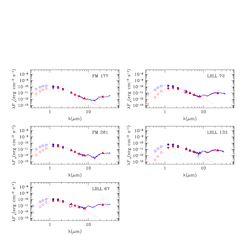
Figure 2.— SEDs of transitional disks in our sample. We show both the observed fluxes (red) and dereddened fluxes (blue; see Table 3 for A_V). In the NIR the emission is similar to that of the stellar photosphere (broken magenta line; Kenyon & Hartmann (1995)), but rises in the MIR and at longer wavelengths. This indicates that the dust in the inner disk has been removed and that there is a hole in the disk. Open circles correspond to ground-based U-, B-, V-, R-, I-, and L-band photometry; closed circles are 2MASS J-, H-, and K-band photometry; triangles are Spitzer IRAC and MIPS photometry. See Section 3.1 for data references. Solid lines are Spitzer IRS spectra from this work. (A color version of this figure is available in the online journal.)

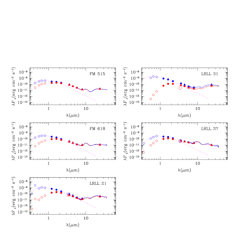
Figure 3.— SEDs of pre-transitional disks in our sample. For LRLL 31, FM 515, and FM 618, there is significant NIR emission above the stellar photosphere, but there is also a dip in the MIR emission and the flux increases at longer wavelengths. This indicates a gap at intermediate radii in the disk. In the case of LRLL 37, there is no clear “dip” in the emission; this object was classified as a pre-transitional disk based on its strong silicate emission which could not be reproduced with a full disk model (see Section 3.3). We classify LRLL 21 as a PTD here even though its NIR excess is weak in this epoch; Flaherty et al. (2012) find that LRLL 21 has significant NIR blackbody emission in more recent IRS observations. The color scheme, symbols, and lines are the same as in Figure 2. (A color version of this figure is available in the online journal.)

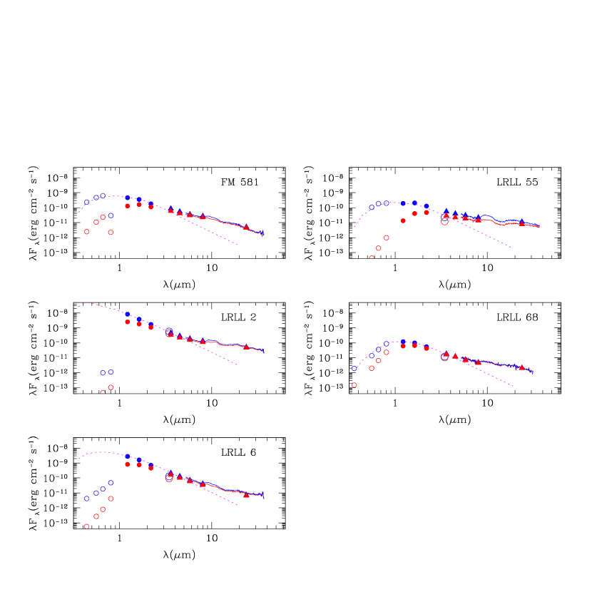
Figure 4.— SEDs of full disks in our sample. The emission decreases at all wavelengths. The color scheme, symbols, and lines are the same as those used in Figure 2. (A color version of this figure is available in the online journal.)

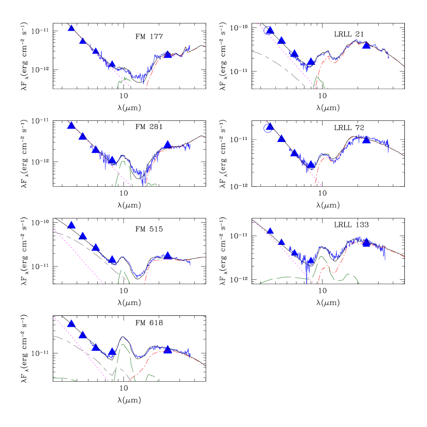
Figure 5.— IR SEDs and disk models (solid, black lines) of transitional and pre-transitional disks in our sample. Here we show only the dereddened data from Figures 2 and 3. Refer to Section 3.3 and Table 4 for model details. Separate model components are the stellar photosphere (magenta dotted line), the inner wall (gray short-long-dashed line), the outer wall (red dot-short-dashed line), and the optically thin small dust located within the inner disk (green long-dashed line). (A color version of this figure is available in the online journal.)

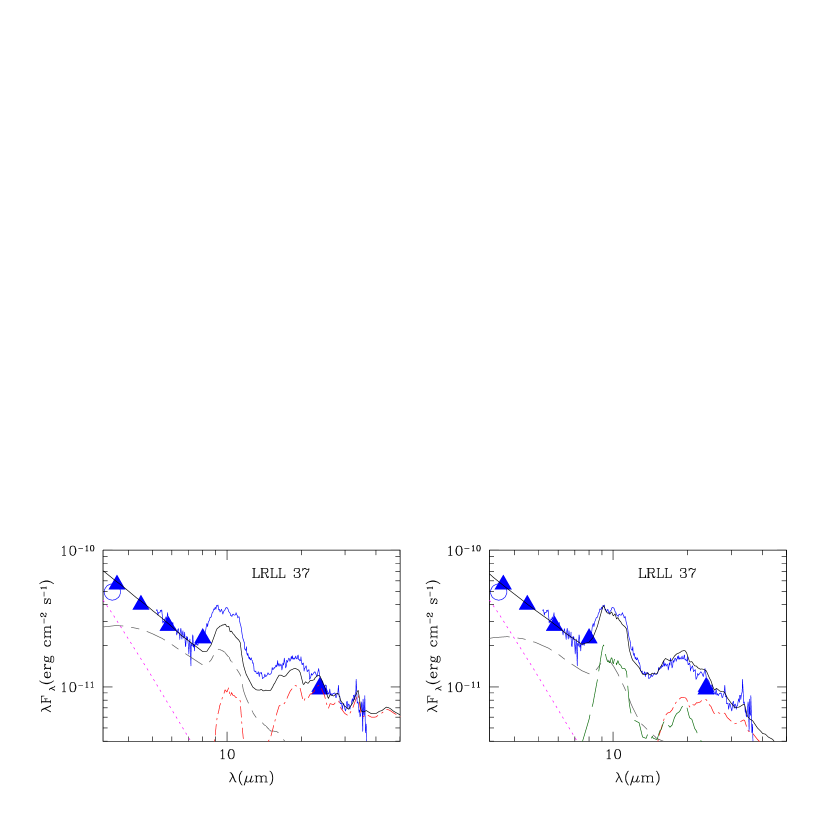
Figure 6.— Left: IR SED and full disk model fit of LRLL 37. We cannot successfully reproduce the 10 $\mu$m and 20 $\mu$m emission. This disk model has ${\epsilon}$=0.001, ${\alpha}$=0.0008, and a_max=0.25$\mu$m. Right: IR SED and pre-transitional disk model of LRLL 37. We can fit the strong silicate emission with a model that has a gap in the disk with most of the silicate emission arising from small, optically thin dust within the gap. The color scheme, symbols, and lines are the same as in Figure 2. (A color version of this figure is available in the online journal.)

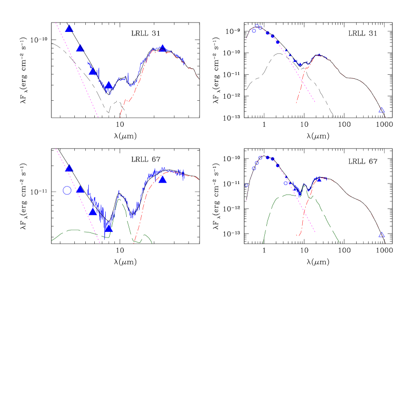
Figure 7.— Left: IR SEDs and disk models of the pre-transitional disk LRLL 31 and the transitional disk LRLL 67. Right: Broad-band SEDs and disk models of LRLL 31 and LRLL 67 which include SMA millimeter data (from this work). With millimeter data we can constrain the outer disk and so we include both the outer wall and the disk behind it in the model presented here (red dot-short-dash). We also show the contribution to the SED from the inner wall of LRLL 31 (gray short-long-dash) and the optically thin small dust located within the inner hole of LRLL 67 (green long-dash). Other symbols and lines are the same as used in Figure 2. (A color version of this figure is available in the online journal.)

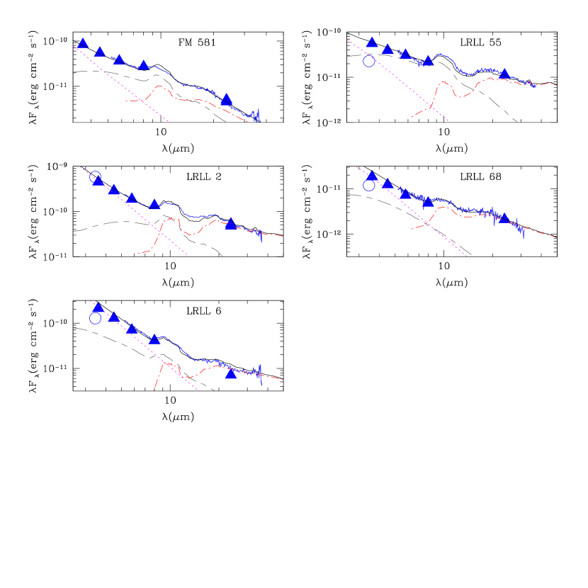
Figure 8.— IR SEDs and disk models of full disks in our sample. We can explain all of these disks with irradiated accretion disk models which incorporate dust settling. In the case of FM 581, we need to truncate the outer disk radius to $<$1 AU in order to reproduce its very steep slope. Refer to Section 3.3 and Table 4 for model details. Here we show the contribution to the SED from the stellar photosphere (magenta dotted line), the inner wall (gray short-long-dash), and the outer disk (red dot-short-dash). (A color version of this figure is available in the online journal.)

Figure 9.— Disk model fits to the SED of LRLL 68 with $\epsilon$$/$$\alpha$=6. Models with the same $\epsilon$-to-$\alpha$ ratio will have similar emission in the IR but substantially different emission in the millimeter. Here we show the following models from Table 5: Model 1 ($\epsilon$=0.0001; short-dashed line), Model 2 ($\epsilon$=0.001; dotted line), and Model 3 ($\epsilon$=0.01; long-dashed line). Note that each model falls below the millimeter upper limit presented in this work (open triangle). This reflects the need for millimeter detections to constrain disk models. (A color version of this figure is available in the online journal.)

Figure 10.— Disk models of LRLL 68 with different R_d, keeping $\epsilon$ and $\alpha$ fixed. Varying the outer radius of the disk will lead to changes in the disk mass, but small changes in the millimeter flux. Models shown are from Table 5: Model 4 (R_d=300 AU; short- long-dashed line), Model 2 (R_d=100 AU; dotted line), and Model 5 (R_d=20 AU; dot- long-dashed line). (A color version of this figure is available in the online journal.)

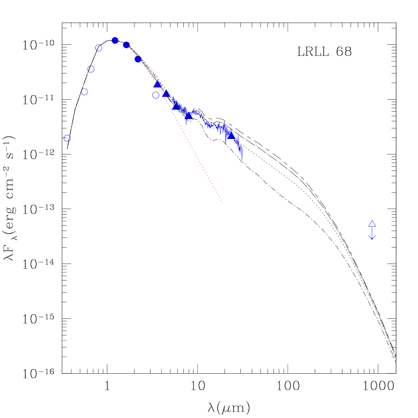
Figure 11.— Disk models of LRLL 68 with different $i$. We find that changing the inclination of the disk, while keeping all other parameters fixed, will lead to substantial differences in the IR emission, but will not significantly affect the millimeter flux. In order of increasing inclination (i.e. from nearly face-on to nearly edge-on) we show the following models from Table 5: Model 6 ($i$=20^∘; short-long-dashed line), Model 7 ($i$=40^∘; dot-long-dashed line), Model 4 ($i$=60^∘; dotted line), Model 8 ($i$=80^∘; dot- short-dashed line). (A color version of this figure is available in the online journal.)

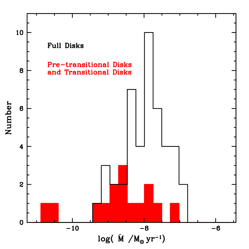
Figure 12.— Distribution of mass accretion rates for Taurus, Chamaeleon, and NGC 2068. We separate full disks (white area) and transitional and pre-transitional disks (shaded area); overall, transitional and pre-transitional disks have lower mass accretion rates than full disks. (A color version of this figure is available in the online journal.)

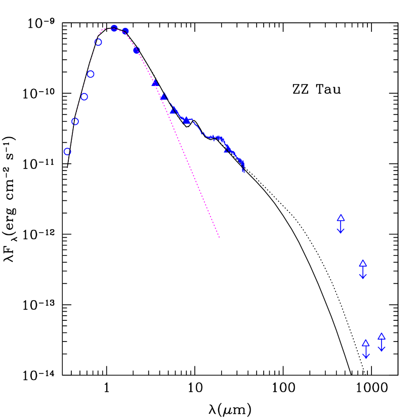
Figure 13.— Models of ZZ Tau using an irradiated accretion disk with dust settling. We show a disk with amorphous silicates and an outer radius of 3 AU (solid) and 100 AU (broken). The color scheme, symbols, and lines are the same as in Figures 2 and 8. U-,B-, V-, R-, and I- photometry are from Kenyon & Hartmann (1995); J-, H-, and K-band data are from Skrutskie et al. (2006); Spitzer IRAC and MIPS data are from Luhman et al. (2010) and the IRS spectrum is from Furlan et al. (2006). All millimeter upper limits are taken from Jensen et al. (1994) and Andrews & Williams (2005). (A color version of this figure is available in the online journal.)

Figure 14.— Rosseland mean optical depth of ZZ Tau for the model shown in Figure 13. ZZ Tau is optically thick to its own radiation ($\tau_{Ross}$$>$1) out to $\sim$1 AU in the disk. It is these innermost disk radii that dominate the emission seen in the IRS spectrum.

References

- Andrews & Williams (2005) Andrews, S. M., & Williams, J. P. 2005, ApJ, 631, 1134
- Andrews et al. (2011) Andrews, S. M., Wilner, D. J., Espaillat, C., Hughes, A. M., Dullemond, C. P., McClure, M. K., Qi, C., & Brown, J. M. 2011, ApJ, 732, 42
- Andrews et al. (2009) Andrews, S. M., Wilner, D. J., Hughes, A. M., Qi, C., & Dullemond, C. P. 2009, ApJ, 700, 1502
- Andrews et al. (2010) —. 2010, ApJ, 723, 1241
- Artymowicz & Lubow (1994) Artymowicz, P., & Lubow, S. H. 1994, ApJ, 421, 651
- Barrado y Navascués & Martín (2003) Barrado y Navascués, D., & Martín, E. L. 2003, AJ, 126, 2997
- Batalha & Basri (1993) Batalha, C. C., & Basri, G. 1993, ApJ, 412, 363
- Bernstein et al. (2003) Bernstein, R., Shectman, S. A., Gunnels, S. M., Mochnacki, S., & Athey, A. E. 2003, in Society of Photo-Optical Instrumentation Engineers (SPIE) Conference Series, Vol. 4841, Society of Photo-Optical Instrumentation Engineers (SPIE) Conference Series, ed. M. Iye & A. F. M. Moorwood, 1694–1704
- Birnstiel et al. (2011) Birnstiel, T., Ormel, C. W., & Dullemond, C. P. 2011, A&A, 525, A11+
- Calvet et al. (2005a) Calvet, N., Briceño, C., Hernández, J., Hoyer, S., Hartmann, L., Sicilia-Aguilar, A., Megeath, S. T., & D’Alessio, P. 2005a, AJ, 129, 935
- Calvet et al. (2002) Calvet, N., D’Alessio, P., Hartmann, L., Wilner, D., Walsh, A., & Sitko, M. 2002, ApJ, 568, 1008
- Calvet & Gullbring (1998) Calvet, N., & Gullbring, E. 1998, ApJ, 509, 802
- Calvet et al. (1991) Calvet, N., Patino, A., Magris, G. C., & D’Alessio, P. 1991, ApJ, 380, 617
- Calvet et al. (2005b) Calvet, N., et al. 2005b, ApJ, 630, L185
- Cieza et al. (2010) Cieza, L. A., et al. 2010, ApJ, 712, 925
- Cody & Hillenbrand (2010) Cody, A. M., & Hillenbrand, L. A. 2010, ApJS, 191, 389
- Cohen et al. (2003) Cohen, M., Megeath, S. T., Hammersley, P. L., Martín-Luis, F., & Stauffer, J. 2003, AJ, 125, 2645
- Currie & Sicilia-Aguilar (2011) Currie, T., & Sicilia-Aguilar, A. 2011, ApJ, 732, 24
- D’Alessio et al. (2001) D’Alessio, P., Calvet, N., & Hartmann, L. 2001, ApJ, 553, 321
- D’Alessio et al. (2006) D’Alessio, P., Calvet, N., Hartmann, L., Franco-Hernández, R., & Servín, H. 2006, ApJ, 638, 314
- D’Alessio et al. (1999) D’Alessio, P., Calvet, N., Hartmann, L., Lizano, S., & Cantó, J. 1999, ApJ, 527, 893
- D’Alessio et al. (1998) D’Alessio, P., Canto, J., Calvet, N., & Lizano, S. 1998, ApJ, 500, 411
- D’Alessio et al. (2005) D’Alessio, P., et al. 2005, ApJ, 621, 461
- Dodson-Robinson & Salyk (2011) Dodson-Robinson, S. E., & Salyk, C. 2011, ApJ, 738, 131
- Dullemond & Dominik (2004) Dullemond, C. P., & Dominik, C. 2004, A&A, 417, 159
- Dullemond & Dominik (2005) —. 2005, A&A, 434, 971
- Dullemond et al. (2001) Dullemond, C. P., Dominik, C., & Natta, A. 2001, ApJ, 560, 957
- Espaillat (2009) Espaillat, C. 2009, PhD thesis, University of Michigan
- Espaillat et al. (2007a) Espaillat, C., Calvet, N., D’Alessio, P., Hernández, J., Qi, C., Hartmann, L., Furlan, E., & Watson, D. M. 2007a, ApJ, 670, L135
- Espaillat et al. (2008a) Espaillat, C., Calvet, N., Luhman, K. L., Muzerolle, J., & D’Alessio, P. 2008a, ApJ, 682, L125
- Espaillat et al. (2011) Espaillat, C., Furlan, E., D’Alessio, P., Sargent, B., Nagel, E., Calvet, N., Watson, D. M., & Muzerolle, J. 2011, ApJ, 728, 49
- Espaillat et al. (2007b) Espaillat, C., et al. 2007b, ApJ, 664, L111
- Espaillat et al. (2008b) —. 2008b, ApJ, 689, L145
- Espaillat et al. (2010) —. 2010, ApJ, 717, 441
- Fischer et al. (2011) Fischer, W., Edwards, S., Hillenbrand, L., & Kwan, J. 2011, ApJ, 730, 73
- Flaherty & Muzerolle (2008) Flaherty, K. M., & Muzerolle, J. 2008, AJ, 135, 966
- Flaherty et al. (2011) Flaherty, K. M., Muzerolle, J., Rieke, G., Gutermuth, R., Balog, Z., Herbst, W., Megeath, S. T., & Kun, M. 2011, ApJ, 732, 83
- Flaherty et al. (2012) Flaherty, K. M., Muzerolle, J., Rieke, G., Gutermuth, R., Balog, Z., Herbst, W., Megeath, S. T., & Kun, M. 2012, ApJ, submitted
- Franchini et al. (1998) Franchini, M., Morossi, C., & Malagnini, M. L. 1998, ApJ, 508, 370
- Furlan et al. (2006) Furlan, E., et al. 2006, ApJS, 165, 568
- Furlan et al. (2009) —. 2009, ApJ, 703, 1964
- Furlan et al. (2011) —. 2011, ApJS, 195, 3
- Goldreich & Tremaine (1980) Goldreich, P., & Tremaine, S. 1980, ApJ, 241, 425
- Gullbring et al. (1998) Gullbring, E., Hartmann, L., Briceno, C., & Calvet, N. 1998, ApJ, 492, 323
- Haisch et al. (2001) Haisch, Jr., K. E., Lada, E. A., & Lada, C. J. 2001, AJ, 121, 2065
- Hartigan et al. (1989) Hartigan, P., Hartmann, L., Kenyon, S., Hewett, R., & Stauffer, J. 1989, ApJS, 70, 899
- Hartmann et al. (1998) Hartmann, L., Calvet, N., Gullbring, E., & D’Alessio, P. 1998, ApJ, 495, 385
- Herbig (1998) Herbig, G. H. 1998, ApJ, 497, 736
- Hernández et al. (2010) Hernández, J., Morales-Calderon, M., Calvet, N., Hartmann, L., Muzerolle, J., Gutermuth, R., Luhman, K. L., & Stauffer, J. 2010, ApJ, 722, 1226
- Hernández et al. (2007) Hernández, J., et al. 2007, ApJ, 671, 1784
- Higdon et al. (2004) Higdon, S. J. U., et al. 2004, PASP, 116, 975
- Houck et al. (2004) Houck, J. R., et al. 2004, ApJS, 154, 18
- Houdebine et al. (1996) Houdebine, E. R., Mathioudakis, M., Doyle, J. G., & Foing, B. H. 1996, A&A, 305, 209
- Huélamo et al. (2011) Huélamo, N., Lacour, S., Tuthill, P., et al. 2011, A&A, 528, L7
- Hughes et al. (2007) Hughes, A. M., Wilner, D. J., Calvet, N., D’Alessio, P., Claussen, M. J., & Hogerheijde, M. R. 2007, ApJ, 664, 536
- Hughes et al. (2009) Hughes, A. M., et al. 2009, ApJ, 698, 131
- Ingleby et al. (2011) Ingleby, L., Calvet, N., Hernández, J., Briceño, C., Espaillat, C., Miller, J., Bergin, E., & Hartmann, L. 2011, AJ, 141, 127
- Ingleby & et al. (2011) Ingleby, L., & et al. 2011, submitted to ApJ
- Isella et al. (2010) Isella, A., Carpenter, J. M., & Sargent, A. I. 2010, ApJ, 714, 1746
- Isella & Natta (2005) Isella, A., & Natta, A. 2005, A&A, 438, 899
- Jensen et al. (1994) Jensen, E. L. N., Mathieu, R. D., & Fuller, G. A. 1994, ApJ, 429, L29
- Jordi et al. (2006) Jordi, K., Grebel, E. K., & Ammon, K. 2006, A&A, 460, 339
- Kenyon & Hartmann (1995) Kenyon, S. J., & Hartmann, L. 1995, ApJS, 101, 117
- Kraus et al. (2011) Kraus, A. L., Ireland, M. J., Martinache, F., & Hillenbrand, L. A. 2011, ApJ, 731, 8
- Kraus et al. (2011) Kraus, A. L., & Ireland, M. J., ApJ, in press
- Lada et al. (2006) Lada, C. J., et al. 2006, AJ, 131, 1574
- Landolt (1992) Landolt, A. U. 1992, AJ, 104, 340
- Lebouteiller et al. (2010) Lebouteiller, V., Bernard-Salas, J., Sloan, G. C., & Barry, D. J. 2010, PASP, 122, 231
- Lima et al. (2010) Lima, G. H. R. A., Alencar, S. H. P., Calvet, N., Hartmann, L., & Muzerolle, J. 2010, A&A, 522, A104+
- Lubow & D’Angelo (2006) Lubow, S. H., & D’Angelo, G. 2006, ApJ, 641, 526
- Luhman et al. (2010) Luhman, K. L., Allen, P. R., Espaillat, C., Hartmann, L., & Calvet, N. 2010, ApJS, 186, 111
- Luhman et al. (2003) Luhman, K. L., Stauffer, J. R., Muench, A. A., Rieke, G. H., Lada, E. A., Bouvier, J., & Lada, C. J. 2003, ApJ, 593, 1093
- Mathis (1990) Mathis, J. S. 1990, ARA&A, 28, 37
- Mathis et al. (1977) Mathis, J. S., Rumpl, W., & Nordsieck, K. H. 1977, ApJ, 217, 425
- McClure (2009) McClure, M. 2009, ApJ, 693, L81
- McClure et al. (2008) McClure, M. K., et al. 2008, ApJ, 683, L187
- Merín et al. (2010) Merín, B., et al. 2010, ApJ, 718, 1200
- Miyake & Nakagawa (1995) Miyake, K., & Nakagawa, Y. 1995, ApJ, 441, 361
- Muzerolle et al. (2010) Muzerolle, J., Allen, L. E., Megeath, S. T., Hernández, J., & Gutermuth, R. A. 2010, ApJ, 708, 1107
- Muzerolle et al. (1998) Muzerolle, J., Calvet, N., & Hartmann, L. 1998, ApJ, 492, 743
- Muzerolle et al. (2003) Muzerolle, J., Calvet, N., Hartmann, L., & D’Alessio, P. 2003, ApJ, 597, L149
- Najita et al. (2007) Najita, J. R., Strom, S. E., & Muzerolle, J. 2007, MNRAS, 378, 369
- Natta et al. (2004) Natta, A., Testi, L., Muzerolle, J., Randich, S., Comerón, F., & Persi, P. 2004, A&A, 424, 603
- Olofsson et al. (2011) Olofsson, J., Benisty, M., Augereau, J.-C., et al. 2011, A&A, 528, L6
- Owen et al. (2011) Owen, J. E., Ercolano, B., & Clarke, C. J. 2011, MNRAS, 412, 13
- Paardekooper & Mellema (2004) Paardekooper, S.-J., & Mellema, G. 2004, A&A, 425, L9
- Pott et al. (2010) Pott, J.-U., Perrin, M. D., Furlan, E., et al. 2010, ApJ, 710, 265
- Quillen et al. (2004) Quillen, A. C., Blackman, E. G., Frank, A., & Varnière, P. 2004, ApJ, 612, L137
- Rice et al. (2003) Rice, W. K. M., Wood, K., Armitage, P. J., Whitney, B. A., & Bjorkman, J. E. 2003, MNRAS, 342, 79
- Rigliaco et al. (2011) Rigliaco, E., Natta, A., Randich, S., Testi, L., Covino, E., Herczeg, G., & Alcalá, J. M. 2011, A&A, 526, L6+
- Robitaille et al. (2007) Robitaille, T. P., Whitney, B. A., Indebetouw, R., & Wood, K. 2007, ApJS, 169, 328
- Sargent et al. (2009) Sargent, B. A., Forrest, W. J., Tayrien, C., et al. 2009, ApJ, 690, 1193
- Schaefer et al. (2006) Schaefer, G. H., Simon, M., Beck, T. L., Nelan, E., & Prato, L. 2006, AJ, 132, 2618