An Arbitrary Curvilinear Coordinate Method for Particle-In-Cell Modeling

Abstract

A new approach to the kinetic simulation of plasmas in complex geometries, based on the Particle-in- Cell (PIC) simulation method, is explored. In the two dimensional (2d) electrostatic version of our method, called the Arbitrary Curvilinear Coordinate PIC (ACC-PIC) method, all essential PIC operations are carried out in 2d on a uniform grid on the unit square logical domain, and mapped to a nonuniform boundary-fitted grid on the physical domain. As the resulting logical grid equations of motion are not separable, we have developed an extension of the semi-implicit Modified Leapfrog (ML) integration technique to preserve the symplectic nature of the logical grid particle mover. A generalized, curvilinear coordinate formulation of Poisson’s equations to solve for the electrostatic fields on the uniform logical grid is also developed. By our formulation, we compute the plasma charge density on the logical grid based on the particles’ positions on the logical domain. That is, the plasma particles are weighted to the uniform logical grid and the self-consistent mean electrostatic fields obtained from the solution of the logical grid Poisson equation are interpolated to the particle positions on the logical grid. This process eliminates the complexity associated with the weighting and interpolation processes on the nonuniform physical grid and allows us to run the PIC method on arbitrary boundary-fitted meshes.

1 INTRODUCTION

The standard Particle-in-Cell (PIC) method utilizes macroparticles to follow the phase space evolution of weakly coupled (collisionless) plasmas. In this regime, PIC can be thought of as an approximate method of integration for the Vlasov equation [1]:

$$\frac{\partial f_{s}}{\partial t}+\vec{v}\cdot\nabla_{\vec{x}}f_{s}+\frac{q_{s}}{m_{s}}(\vec{E}+\vec{v}\times\vec{B})\cdot\nabla_{\vec{v}}f_{s}=0,$$ (1)

where $f_{s}(\vec{x},\vec{v},t)$ is the time-dependent six-dimensional phase space distribution function of the plasma particles of species $s$. For simplicity, in this work we limit ourselves to the electrostatic case with no applied background magnetic field. Applying the method of characteristics [2] to (1), it can therefore be shown that the PIC macroparticle orbits evolve self-consistently in phase-space according to

$$\begin{array}[]{rcl}\dot{\vec{x}}&=&\vec{v}\\ \dot{\vec{v}}&=&-\frac{q_{M}}{m_{M}}\nabla\Phi(\vec{x}).\end{array}$$ (2)

In (2), an overdot denotes a time derivative and the macroparticle charge and mass satisfy $q_{M}/m_{M}=q_{s}/m_{s}$. The mean-field electrostatic potential $\Phi(\vec{x})$ is obtained on a computational mesh via Poisson’s equation

$$\nabla^{2}\Phi(\vec{x})=-4\pi\rho(\vec{x})=-4\pi\sum_{i=1}^{N_{M}}q_{M}S(\vec{x}-\vec{x_{i}}).$$ (3)

In our notation, $N_{M}$ is the number of macroparticles (assumed to be of the same species with equal charge for simplicity) and $\vec{x}_{i}$ are the particle positions. $\rho(\vec{x})$ is the charge density obtained at discrete locations on the mesh from the macroparticles at $\vec{x}_{i}$ using interpolation functions, $S(\vec{x}-\vec{x_{i}})$, typically chosen to be $B$-splines [3]. These interpolation functions effectively give the macroparticles a finite width based upon the grid spacing and lead to cutoff Coulombic interactions between macroparticles [4].

PIC codes are generally designed using rectangular meshes in Cartesian geometry, but have been extended to cylindrical and spherical coordinates. However, extension to arbitrary grids has proven much more difficult. Jones [5] was among the first to develop a curvilinear-coordinate PIC method capable of operating on boundary-conforming grids tailored to accelerator and pulsed-power applications. Other codes were soon developed in an effort to model ion diodes [6, 7] and microwave devices [8] more accurately. These early methods involved generating a nonuniform initial grid based upon the physical boundaries of the system and running the PIC components on this physical grid. There are many benefits to this type of system, such as having smoothly curved boundaries in contrast to the “stair-stepped” boundaries inherent to the rectangular-grid PIC approach, which occur when a part of the boundary is not aligned with either coordinate surface. Furthermore, higher grid density can be placed in areas of interest within the system either statically or by allowing the grid to adapt dynamically [9, 10] to the problem by following a pre-specified control function. Implemented wisely, such techniques should allow complex geometries to be simulated at a fraction of the cost associated with using a uniform grid code, in which the entire mesh must have the resolution required to resolve the smallest physical features of the system, and in which the grid does not conform to the boundary.

Arbitrary grid methods are not without their problems. Nonuniform grid cells make it computationally expensive to locate macroparticles on the grid for the charge accumulation and field interpolation steps of the PIC method, as well as for enforcing the particle boundary conditions. In a standard PIC code with a uniform structured grid, particle positions on the grid are easily determined. On a nonuniform grid, this location must be done iteratively [11], which increases the computational cost of the method. Furthermore, interpolation on a nonuniform grid is complicated by the variations of the grid, which change the shape of the interpolation functions, often in a non-trivial way [12]. Finally, as the ratio of the largest to the smallest cell size increases and the number of particles per cell in the smallest cells becomes small, the amount of noise near the small cells also increases (assuming the charge density is roughly constant). Thus, complex and often time-consuming gridding strategies [13] and/or particle splitting and merging algorithms [14] must be implemented to keep the noise within the system to a minimal threshold value while the structures of interest within the system are still resolved.

We consider the problems associated with these and other existing adaptive grid PIC approaches to be serious. As such, we have developed a new nonuniform grid PIC method, which incorporates some of the best features of several existing methods with a new idea for the implementation of the PIC method. Our goal is to design an arbitrary, curvilinear-coordinate PIC (ACC-PIC) code capable of operating efficiently and accurately on an arbitrary (but structured) moving mesh for a boundary of arbitrary geometry. We construct a logical (or computational) grid on the unit square and map it to the physical domain, as illustrated in Figure 1. We implement the main components of the PIC method–the charge accumulation, particle push, field solve, and interpolation–on this logical domain. This approach deals with all the problems listed in the previous paragraph except the last. The issue of having some cells with much fewer macroparticles than others is still a problem requiring attention, for example particle splitting and merging.

In this paper, we present results on the development of these methods into a 2D, electrostatic PIC code. By implementing the PIC components on the logical grid, we show that we can eliminate the particle location and interpolation problems that plagued the earlier boundary conforming non-uniform grid methods [5, 6, 7, 8]. Particle locations are easily found on the logical grid using the same techniques as standard uniform grid PIC codes. Since the charge accumulation and field interpolation are both done on the logical grid, we are again able to use the efficient algorithms that are utilized in a uniform grid code. This eliminates the need for calculating non-standard particle shapes on the physical grid [12]. Furthermore, we develop a Hamiltonian-based, semi-implicit second-order accurate symplectic logical grid mover and apply it to the time advance of the particles that includes the effects of inertial forces. This mover has the important property of requiring only a single field solve per timestep. Since we are moving particles on a square grid, particle boundary conditions, which may be difficult to implement on a nonuniform physical grid, are fairly simple with our approach. Finally, our method allows us to solve the electrostatic field equations on a simple square mesh in the logical domain rather than in the complex physical domain.

The remainder of this paper is structured as follows. In Section 2, we quickly review the Winslow method of generating a grid that conforms to a curved boundary, with finer grid near parts of the boundary with more curvature. We derive the particle equations of motion on the logical grid in Section 3, and discuss the semi-implicit modified leapfrog integration technique utilized for the integration of these equations in Section 4. Section 5 describes the solution of the electrostatic field equations on the logical grid, as well as details of the charge weighting/field interpolation schemes utilized. We perform several standard tests for the verification of our 2D, electrostatic, nonuniform grid PIC code in Section 7. Finally, we present our conclusions and suggestions for future work on the method in Section 8. A general overview of our differential geometry notation is given in A, and a derivation of the Poisson equation in logical space is given in B.

2 Logical to Physical Grid Mapping

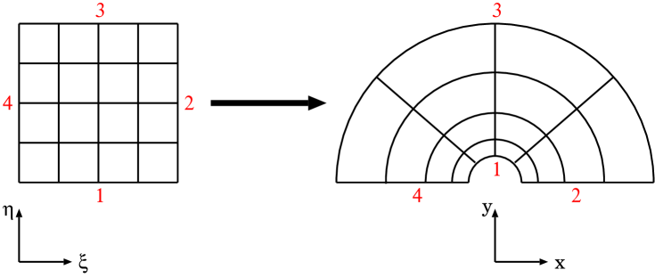
Figure 1: Schematic for mapping from the logical to the physical grid for an annulus. The numbers along the boundaries of the square logical domain are used to indicate which edge of the square maps to which boundary segment on the physical domain.

2.1 Grid Generation Technique

For completeness, we include here a discussion of Winslow’s Laplace method [15], a simple grid generation technique which illustrates the logical to physical grid mapping inherent to this work. In Winslow’s method, a set of uncoupled Laplace equations are solved on a uniform square 2D logical domain, $\xi,\eta\in[0:1]$. With Winslow’s method, the finest gridding is concentrated in the regions of highest boundary curvature, e.g. around an object at the center of the domain. (See Figure 1, in which the surface labeled “$1$” might represent a dust grain, “$3$” represents an artificial boundary far away, and symmetry is imposed on surfaces “$2$” and “$4$.” As discussed in Section 5, this figure can represent either azimuthal or axial symmetry.) While this gridding method is rather primitive in that we have no control over where the grid is concentrated away from the boundary, we have chosen this method for its simplicity and suitability for illustrating the feasibility of our ACC-PIC method. Winslow’s method provides a simple way of generating an initial boundary conforming grid, to be adapted to the solution at later timesteps, while still retaining conformation to the boundary using more sophisticated techniques.

The Laplace equation can be written in any coordinate system, but for simplicity we have chosen to implement Winslow’s method in the Cartesian coordinate system in physical space. In the physical domain, Laplace’s equation takes the form

$$\nabla_{x}^{2}\xi^{\alpha}=\frac{\partial}{\partial x^{\beta}}\frac{\partial\xi^{\alpha}}{\partial x^{\beta}}=0,\quad\alpha,\beta=1,\cdots,n.$$ (4)

In (4), the logical variables $\xi^{\alpha}$ are the dependent variables and the physical variables $x^{\beta}$ are the independent variables. Here and in the rest of this paper we assume summation over repeated indices. However, since we would prefer to solve the Laplace equation on the uniform logical space $(\xi,\eta)$ rather than directly gridding (4) on the physical domain, solving for $\xi(x,y),\eta(x,y)$ and inverting, we must transform the set of PDE’s such that $x^{\beta}$ are the dependent variables and $\xi^{\alpha}$ are the independent variables. This transformation has been outlined by Liseikin [16]; a detailed derivation can be found in [17]. After much manipulation, we write the final system of equations to be solved as

$$\begin{array}[]{rcl}g_{22}\frac{\partial^{2}x}{\partial\xi^{2}}-2g_{12}\frac{\partial^{2}x}{\partial\xi\partial\eta}+g_{11}\frac{\partial^{2}x}{\partial\eta^{2}}&=&0\\ g_{22}\frac{\partial^{2}y}{\partial\xi^{2}}-2g_{12}\frac{\partial^{2}y}{\partial\xi\partial\eta}+g_{11}\frac{\partial^{2}y}{\partial\eta^{2}}&=&0,\end{array}$$ (5)

where

$$g_{\mu\nu}(\vec{\xi}\,)\equiv\frac{\partial x^{\gamma}}{\partial\xi^{\mu}}\frac{\partial x^{\gamma}}{\partial\xi^{\nu}},\quad\mu,\nu,\gamma=1,\cdots,n$$ (6)

is the covariant metric tensor (see Appendix A). While (5)(a) and (b) appear to be the same equation for $x(\xi,\eta)$ and for $y(\xi,\eta)$, they actually possess opposite boundary conditions along each segment of the grid boundary: For any segment of the boundary, we have Neumann boundary conditions for $\xi$ and Dirichlet boundary conditions for $\eta$ or vice-versa, both expressed in terms of $x(\xi,\eta)$ and $y(\xi,\eta)$. Furthermore, from (4) and these boundary conditions, we know that $\xi(x,y)$ and $\eta(x,y)$ are conjugate harmonic functions. Thus, Winslow’s method forces the grid lines to be orthogonal (i.e. $g_{12}=0$) in the physical space.

Since the covariant terms $g_{\alpha\beta}$ depend on $\frac{\partial x_{\alpha}}{\partial\xi_{\beta}}$ and the solution we seek is $x(\xi,\eta),y(\xi,\eta)$, the system of equations is nonlinear. (5) are therefore discretized using a second-order accurate finite-difference method and, because of their non-linear form, are iteratively solved using an inexact Newton-Krylov solver with the Generalized Minimal Residual Method (GMRES) [18, 19].

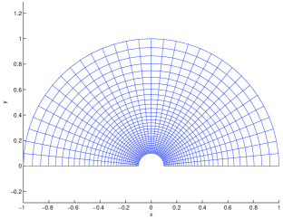
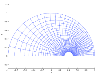
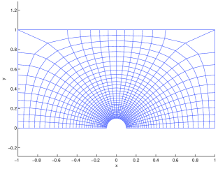
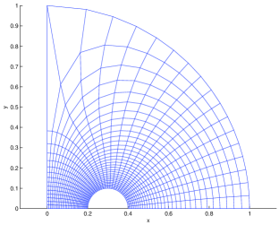
Figure 2: Grids generated using Winslow’s method with a circular object along the inner physical grid boundary, symmetry along the bottom segments (and on the left in (d)), and an artificial boundary far away at top. Here we have used a $32\times 32$ grid in order to show the mapping more clearly. The appearance of nonorthogonal grid lines is due to the straight lines used by the plotting tool.

Winslow grids can be specified for a wide array of physical domains by specifying boundary conditions on boundary segments, as illustrated in Figure 1. The grids presented in Figure 2 are of some of the physical grids with circular objects along the inner boundary which we have generated using Winslow’s method. As we discuss in Section 5, this circular segment can represent a cylindrical or spherical surface. We have also generated grids with elliptically shaped objects, and are capable of generating objects of fairly general shape and size on any boundary segment [17].

3 DEVELOPMENT OF LOGICAL GRID EQUATIONS OF MOTION

The most obvious method for implementing our mover in logical space would seem to be by simply converting the Newton-Lorentz equations of motion from the physical to the logical grid. Specializing to 1d for simplicity and defining $u=\dot{\xi}=v/J$, we recast (2) as

$$\begin{array}[]{rcl}\dot{\xi}&=&f(u)=u\\ \dot{u}&=&g(\xi,u)=-\frac{J^{\prime}u^{2}}{J}-\frac{q}{m}\frac{1}{J^{2}}\Phi^{\prime},\end{array}$$ (7)

where $J\equiv\frac{dx}{d\xi}$ in 1d and the prime symbol represents a derivative with respect to the logical coordinate $\xi$. For compactness we have dropped the subscripts designating macroparticle quantities here and in the rest of this paper. Taking the formal divergence of (7), we have

$$\frac{\partial f}{\partial\xi}\bigg{|}_{u}+\frac{\partial g}{\partial u}\bigg{|}_{\xi}=-\frac{2J^{\prime}u}{J}\neq 0.$$ (8)

The Newton-Lorentz equations of motion are therefore not divergence-free in these variables. As such, a time integration of these equations of motion with a standard “naive” leapfrog (LF) integrator,

$$\begin{array}[]{rcl}\xi^{\prime}&=&\xi+\Delta t\,f(u)\\ u^{\prime}&=&u+\Delta t\,g(\xi^{\prime},u),\end{array}$$ (9)

will not preserve phase space area, and the particle orbits will typically spiral inward or outward with time [17].

3.1 Hamiltonian Approach to Logical Grid Equations of Motion

Clearly, since the system of equations in (7) are not in a canonical Hamiltonian formulation, transformation of the Newton-Lorentz equations of motion into logical coordinates leads to a lack of $(\xi,u)$ phase space area conservation. We therefore construct logical grid particle equations of motion based on Hamilton’s equations by using a canonical transformation $(\vec{x},\vec{p})\rightarrow(\vec{\xi},\vec{P})$, where $p^{\alpha}=mv^{\alpha}$ is the physical space momentum and $P^{\alpha}$ is the logical space momentum. This transformation is constructed via an $F_{2}(\vec{x},\vec{P},t)$ generating function [20], thereby assuring Hamiltonian equations of motion on the logical grid. Under the canonical transformation we have

$$\begin{array}[]{rcl}p^{\alpha}&=&\frac{\partial}{\partial x^{\alpha}}F_{2}(\vec{x},\vec{P},t)\\ \xi^{\alpha}&=&\frac{\partial}{\partial P^{\alpha}}F_{2}(\vec{x},\vec{P},t).\end{array}$$ (10)

We have chosen the $F_{2}$ generating function such that $\vec{x}$ and $\vec{P}$ are considered independent variables. The transformed Hamiltonian $K$ is given by

$$K=H+\frac{\partial F_{2}}{\partial t}.$$ (11)

A time-adaptive grid is beyond the scope of this paper; we therefore drop the second term of (11). Specializing to the contact transformation $\vec{\xi}=\vec{\xi}(\vec{x})$, we write the $F_{2}(\vec{x},\vec{P})$ generating function as

$$F_{2}(\vec{x},\vec{P})=\xi^{\beta}(\vec{x})P^{\beta},$$ (12)

such that by (10), we have $p^{\alpha}=k^{\beta\alpha}P^{\beta}$ and $\xi^{\alpha}=\xi^{\alpha}(\vec{x})$. Here $k^{\beta\alpha}$ is the inverse Jacobi matrix as defined in Appendix A.

In the absence of a static background magnetic field $\vec{B}$, the physical grid Hamiltonian is given in general form by

$$H=\sum_{i}\frac{p_{i}p_{i}}{2m}+q\Phi(\vec{x}),$$ (13)

where the sum is over three rectangular components in physical space. Notice that (13) is fully separable, $H=T(\vec{p})+V(\vec{x})$. In this work, we consider two distinct 2D cases, with azimuthal ($z$) symmetry and axial ($\phi$) symmetry. In the former, the grid segment labeled “$1$” along the curved grid segment in Figure 1 represents, for example, a cylindrical probe. For the axisymmetric case, this segment would represent a spherical probe. We stress here that both cases lead to separable Hamiltonians in the physical domain.

(13) can then be used in conjunction with ( 11) to construct the logical grid Hamiltonian:

$$K=\frac{1}{2m}\left(g^{\beta\gamma}P^{\beta}P^{\gamma}\right)+V(\vec{\xi}),$$

where $g^{\beta\gamma}$ is the contravariant metric tensor as defined in (52). Again, since $g^{\beta\gamma}=g^{\beta\gamma}(\xi,\eta)$, we must represent $g^{\beta\gamma}$ in terms of the covariant metric tensor as in (54). Note that on the logical grid the transformed Hamiltonian can be written $K=T(\vec{\xi},\vec{P})+V(\vec{\xi})$, meaning that we have transformed the separable physical grid Hamitonian to an equivalent, but non-separable system. Applying Hamilton’s equations, $\dot{\xi}^{\alpha}\equiv\frac{\partial K}{\partial P^{\alpha}}$ and $\dot{P}^{\alpha}\equiv-\frac{\partial K}{\partial\xi^{\alpha}}$ to (3.1) gives the logical grid equations of motion:

$$\begin{array}[]{rcl}\dot{\xi}^{\mu}&=&\frac{g^{\gamma\mu}P^{\gamma}}{m}=U^{\mu}(\vec{\xi},\vec{P})\\ \dot{P}^{\mu}&=&-\frac{1}{2m}\frac{\partial g^{\beta\gamma}}{\partial\xi^{\mu}}P^{\beta}P^{\gamma}-\frac{\partial V}{\partial\xi^{\mu}}=W^{\mu}(\vec{\xi},\vec{P}).\end{array}$$ (14)

We note here that the term quadratic in $\vec{P}$ represents the inertial force in these coordinates, and that both $\dot{\xi}^{\mu}$ and $\dot{P}^{\mu}$ are functions of $\xi^{\alpha}$ and $P^{\alpha}$. Since these equations are obtained from a Hamiltonian in canonical variables, the divergence for each degree of freedom $\frac{\partial U^{\mu}}{\partial\xi^{\mu}}+\frac{\partial W^{\mu}}{\partial P^{\mu}}$ (no sum) is zero.

4 PARTICLE PUSH: MODIFIED LEAPFROG INTEGRATOR

Whereas the physical space Hamiltonian leads to separable equations of motion which can be integrated by standard LF integration techniques, in the logical space this is no longer true. Since (14) is not a separable system of equations, integration with the LF method will not conserve phase space area.

As such, we have chosen to implement an extension of the semi-implicit modified leapfrog (ML) integrator originally developed by Finn and Chacón [21] for integrating 2D solenoidal flows in fluid dynamics and magnetic field lines in MHD codes. (Because the dependence of the Hamiltonian on the canonical momentum is given analytically, the exactly divergence free interpolations used in [21] are not necessary.) Rewriting (14) as $\dot{\vec{P}}=\vec{W}$ and $\dot{\vec{\xi}}=\vec{U}$, respectively, and denoting explicit (implicit) updates with a superscript $e$ ($i$), the ML integrator can be written as $\vec{M}_{\Delta t}=\vec{P}^{e}_{\Delta t}\circ\vec{\xi}^{i}_{\Delta t}$, where

$$\vec{\xi}^{i}_{\Delta t}:\left\{\begin{array}[]{c}\vec{\xi}_{1}=\vec{\xi}+\Delta t\,\vec{U}(\vec{\xi}_{1},\vec{P})\\ \vec{P}_{1}=\vec{P}\end{array}\right.,\quad\vec{P}^{e}_{\Delta t}:\left\{\begin{array}[]{c}\vec{\xi}^{\prime}=\vec{\xi}_{1}\\ \vec{P}^{\prime}=\vec{P}_{1}+\Delta t\,\vec{V}(\vec{\xi}_{1},\vec{P}_{1})\end{array}\right..$$ (15)

Combining, we have

$$\begin{array}[]{rcl}\vec{\xi}^{\prime}&=&\vec{\xi}+\Delta t\,\vec{U}(\vec{\xi}^{\prime},\vec{P})\\ \vec{P}^{\prime}&=&\vec{P}+\Delta t\,\vec{V}(\vec{\xi}^{\prime},\vec{P}).\end{array}$$ (16)

The map $\xi^{i}_{\Delta t}$ is implicit and must be done by means of Newton or Picard iterations. The map $P^{e}_{\Delta t}$ is explicit, and can therefore be applied directly. It can be shown that, unlike the standard LF scheme commonly utilized in PIC codes, this non-time-centered formulation of the ML scheme results in only first-order accuracy in $\Delta t$. To achieve second-order accuracy in time, we simply symmetrize the ML scheme by composing $\vec{\xi}^{e}_{\Delta t/2}\circ\vec{P}^{i}_{\Delta t/2}\circ\vec{P}^{e}_{\Delta t/2}\circ\vec{\xi}^{i}_{\Delta t/2}$. As shown in [21], the implicit-followed-by-explicit ordering in each pair of mappings retains the area preserving nature of the integrator in a 2D phase space (one degree of freedom.) This integrator is seen to be symplectic for arbitrary degrees of freedom because it can be derived from a generating function [20]

$$F_{3}(\vec{\xi}^{\prime},\vec{P})=-\xi^{\prime\alpha}P^{\alpha}+\Delta tK(\vec{\xi}^{\prime},\vec{P}),$$ (17)

with

$$\begin{array}[]{rcl}P^{\prime\alpha}&=&-\frac{\partial}{\partial\xi^{\prime\alpha}}F_{3}(\vec{\xi}^{\prime},\vec{P})\\ \xi^{\alpha}&=&-\frac{\partial}{\partial P^{\alpha}}F_{3}(\vec{\xi}^{\prime},\vec{P}).\end{array}$$ (18)

The second half of the ML update ($\vec{P}^{e}_{\Delta t/2}\circ\vec{\xi}^{i}_{\Delta t/2}$) is described by an $F_{2}(\vec{\xi},\vec{P}^{\prime})$ generating function. The alternation of the steps in $\vec{\xi}$ and $\vec{P}$ gives second-order accuracy in $\Delta t$. The logical flow of the ML integrator as implemented on (14) is

$$\vec{\xi}^{i}_{\Delta t/2}\rightarrow\vec{P}^{e}_{\Delta t/2}\rightarrow\vec{P}^{i}_{\Delta t/2}\rightarrow\vec{\xi}^{e}_{\Delta t/2}.$$

We note here that the charge density is accumulated on the grid and the mean field solve is performed after the implicit position update step of the symmetrized ML mover. While this mover requires us to pass through the particle array twice per timestep, it allows us to accumulate the charge density and solve for the fields only once per timestep.

With the exception of the case in Sec. 7.4, the boundary conditions we use are periodic, and we therefore do not need to describe particle reflection in the logical space. Reflecting conditions on particles can be implemented with some care in logical coordinates.

5 FIELD SOLVER: GENERALIZED POISSON EQUATION

In order to solve the electrostatic field equation on the logical grid, we first write the Poisson equation on the physical grid

$$\frac{1}{f}\nabla\cdot f\nabla\Phi=\frac{1}{f}\frac{\partial}{\partial x^{\alpha}}\cdot f\frac{\partial\Phi}{\partial x^{\alpha}}=-4\pi\rho^{x},$$ (19)

where $\rho^{x}$ is the physical charge density. Here, $f$ is a geometry factor. For azimuthal symmetry, $f=1$ and the Poisson equation takes the usual form

$$\nabla^{2}\Phi=-4\pi\rho^{x}.$$ (20a)

For axisymmetry, we have $$f=r$$ and the Poisson equation takes the form

$$\nabla\cdot\left(r\nabla\Phi\right)=-4\pi r\rho^{x}.$$ (20b)

The generalized curvilinear coordinate formulation of Poisson’s equation on the logical grid takes the form

$$\frac{1}{fJ}\frac{\partial}{\partial\xi^{\alpha}}\left(fJg^{\alpha\beta}\frac{\partial\Phi}{\partial\xi^{\beta}}\right)=-4\pi\rho^{x},$$ (21)

as derived in Appendix B. The logical density $\rho^{\xi}$ is equal to $J\rho^{x}$, leading to

$$\frac{\partial}{\partial\xi^{\alpha}}\left(fJg^{\alpha\beta}\frac{\partial\Phi}{\partial\xi^{\beta}}\right)=-4\pi f\rho^{\xi}.$$ (22)

In this form, we accumulate the logical density $\rho^{\xi}$ and solve the Poisson equation by conservative differencing, as described in the next section. This logical grid solver removes the necessity of writing and maintaining multiple complex-geometry Poisson solvers for the various coordinate systems we wish to model.

6 NUMERICAL IMPLEMENTATION

For our 2D code, we have a wide range of grid choices on which to perform validation tests for our method in this and the next section. For the sake of brevity, we outline only two here, both of which have been designed such that analytical expressions for the metric tensors are easily obtained. In addition to the annulus grid generated numerically by the methods described in Section 2, we define a doubly periodic, nonuniform, orthogonal grid using:

$$\begin{array}[]{rcl}x&=&x_{\mathrm{min}}+(x_{\mathrm{max}}-x_{\mathrm{min}})(\xi+\epsilon_{g}\sin{2\pi\xi})\\ y&=&y_{\mathrm{min}}+(y_{\mathrm{max}}-y_{\mathrm{min}})(\eta+\epsilon_{g}\sin{2\pi\eta}).\end{array}$$ (23a)

Here $$x_{\mathrm{min}} x_{\mathrm{max}} y_{\mathrm{min}} y_{\mathrm{max}} \epsilon_{g}$$, , , and are constants to scale boundaries of the physical grid to form a rectangle of arbitrary size. Here, is the nonuniformity parameter which controls the amount of nonuniformity of the grids. A doubly-periodic grid has been chosen for the implementation of the periodic field and particle boundary conditions utilized for the tests in the Section 7. We have also designed a doubly-periodic, nonorthogonal grid given by

$$\begin{array}[]{rcl}x&=&x_{\mathrm{min}}+(x_{\mathrm{max}}-x_{\mathrm{min}})(\xi+\epsilon_{g}\sin{2\pi\xi}\sin{2\pi\eta})\\ y&=&y_{\mathrm{min}}+(y_{\mathrm{max}}-y_{\mathrm{min}})(\eta+\epsilon_{g}\sin{2\pi\xi}\sin{2\pi\eta})\end{array}$$ (23b)

to test the effects of non-zero cross terms ($g^{12}$) in our code, both in the field solver and the particle mover. For simplicity, we have constrained the grid nonuniformity parameter $\epsilon_{g}$ in (23a) and (23b) to be the same in each dimension. Notice that both (23a) and (23b) require that $\epsilon_{g}<\frac{1}{2\pi}$ so that the grid does not fold.

6.1 Discretization of Particle Equations

In two spatial dimensions, the logical grid particle equations of motion ((14)) can be written as

$$\begin{array}[]{rcl}\vphantom{\Biggl{(}}\dot{\xi}&=&\frac{1}{m}\left(g^{11}P_{\xi}+g^{12}P_{\eta}\right)\\ \vphantom{\Bigl{(}}\dot{\eta}&=&\frac{1}{m}\left(g^{12}P_{\xi}+g^{22}P_{\eta}\right),\end{array}$$ (24a)

and

$$\begin{array}[]{rcl}\vphantom{\Biggl{(}}\dot{P}_{\xi}&=&\frac{-1}{2m}\left(P_{\xi}^{2}\frac{\partial g^{11}}{\partial\xi}+2P_{\xi}P_{\eta}\frac{\partial g^{12}}{\partial\xi}+P_{\eta}^{2}\frac{\partial g^{22}}{\partial\xi}\right)-\frac{\partial V(\vec{\xi}\,)}{\partial\xi}\\ \vphantom{\Biggl{(}}\dot{P}_{\eta}&=&\frac{-1}{2m}\left(P_{\xi}^{2}\frac{\partial g^{11}}{\partial\eta}+2P_{\xi}P_{\eta}\frac{\partial g^{12}}{\partial\eta}+P_{\eta}^{2}\frac{\partial g^{22}}{\partial\eta}\right)-\frac{\partial V(\vec{\xi}\,)}{\partial\eta}.\end{array}$$ (24b)

Note that we have written (24) in terms of the contravariant metric tensor, $g^{\mu\nu}=g^{\mu\nu}(\vec{x}\,)$, which is easily obtained as the inverse of the covariant metric tensor, $g_{\mu\nu}(\vec{\xi}\,)$ as in (54).

The third momentum component is generated at $t=0$ and held as a constant as the simulation progresses. This term contributes to the simulation through its inclusion in the effective potential term, $V(\vec{\xi}\,)$. In azimuthal symmetry, $(x_{1},x_{2})=(x,y)$ and the effective potential is $V_{\mathrm{azi}}(\vec{\xi}\,)=\frac{p_{z}^{2}}{2m}+q\Phi(\vec{\xi}\,)$, such that the ignorable-direction momentum does not contribute to the momentum update equations. However, for an axisymmetric problem, $(x_{1},x_{2})=(r,z)$ and the effective potential is $V_{\mathrm{axi}}(\vec{\xi}\,)=\frac{p_{\phi}^{2}}{2mr(\vec{\xi}\,)^{2}}+q\Phi(\vec{\xi}\,)$, such that its derivative is

$$\begin{array}[]{rcl}\vphantom{\Bigl{(}}\frac{\partial V(\vec{\xi}\,)}{\partial\xi}&=&-\frac{j_{11}p_{\phi}^{2}}{mr^{3}}-qE_{\xi}\\ \vphantom{\Biggl{(}}\frac{\partial V(\vec{\xi}\,)}{\partial\eta}&=&-\frac{j_{12}p_{\phi}^{2}}{mr^{3}}-qE_{\eta},\end{array}$$ (25)

where $(x_{1},x_{2})=(r,z)$ implies $j_{11}=\partial r/\partial\xi$ and $j_{12}=\partial r/\partial\eta$. Thus, in the axisymmetric case we must also interpolate the $j_{11}$ and $j_{12}$ components of the Jacobi matrix and the $r$-coordinate of the particle’s physical space position to the particle position on the logical grid.

6.2 Conservative discretization of Poisson equation

In two dimensions the logical grid Poisson equation, (22), takes the form

$$\frac{\partial}{\partial\xi}\left(D^{11}\frac{\partial\Phi}{\partial\xi}+D^{12}\frac{\partial\Phi}{\partial\eta}\right)+\frac{\partial}{\partial\eta}\left(D^{12}\frac{\partial\Phi}{\partial\xi}+D^{22}\frac{\partial\Phi}{\partial\eta}\right)=-4\pi\mathit{f}\rho^{\xi},$$ (26)

where we have defined $D^{\mu\nu}\equiv\mathit{f}Jg^{\mu\nu}$, again written in terms of the contravariant metric tensor $g^{\mu\nu}(\vec{x})$. (26) is comprised of a set of co-directed derivatives proportional to the diagnonal metric tensor components ($D^{11}$ and $D^{22}$) and a set of cross-directed derivatives for the off-diagonal metric tensor components ($D^{12}$), i.e. $\nabla^{2}\Phi=(\nabla^{2}\Phi)^{\mathrm{co}}+(\nabla^{2}\Phi)^{\mathrm{cross}}$, the latter of which are nonzero for non-orthogonal coordinates ($g^{12}\neq 0$). We have defined the coordinates $\xi,\eta$ at vertices $i,j$, thus $\Phi$ and $\rho$ are naturally defined at cell centers $i+1/2,j+1/2$. The co- and cross-directed terms are discretized using appropriate centered-difference schemes, leading to the final discretized form of (26):

$$\begin{array}[]{c}-4\pi\mathit{f}\rho^{\xi}_{i+\frac{1}{2},j+\frac{1}{2}}=\\ \frac{D^{11}_{i+1,j+\frac{1}{2}}\left(\Phi_{i+\frac{3}{2},j+\frac{1}{2}}-\Phi_{i+\frac{1}{2},j+\frac{1}{2}}\right)-D^{11}_{i,j+\frac{1}{2}}\left(\Phi_{i+\frac{1}{2},j+\frac{1}{2}}-\Phi_{i-\frac{1}{2},j+\frac{1}{2}}\right)}{\Delta\xi^{2}}+\\ \par\frac{D^{22}_{i+\frac{1}{2},j+1}\left(\Phi_{i+\frac{1}{2},j+\frac{3}{2}}-\Phi_{i+\frac{1}{2},j+\frac{1}{2}}\right)-D^{22}_{i+\frac{1}{2},j}\left(\Phi_{i+\frac{1}{2},j+\frac{1}{2}}-\Phi_{i+\frac{1}{2},j-\frac{1}{2}}\right)}{\Delta\eta^{2}}+\\ \par\frac{1}{4\,\Delta\xi\,\Delta\eta}\left[D^{12}_{i+1,j+1}\left(\Phi_{i+\frac{3}{2},j+\frac{3}{2}}-\Phi_{i+\frac{1}{2},j+\frac{1}{2}}\right)-D^{12}_{i,j}\left(\Phi_{i+\frac{1}{2},j+\frac{1}{2}}-\Phi_{i-\frac{1}{2},j-\frac{1}{2}}\right)+\right.\\ \left.D^{12}_{i+1,j}\left(\Phi_{i+\frac{1}{2},j+\frac{1}{2}}-\Phi_{i+\frac{3}{2},j-\frac{1}{2}}\right)+D^{12}_{i,j+1}\left(\Phi_{i-\frac{1}{2},j+\frac{3}{2}}-\Phi_{i+\frac{1}{2},j+\frac{1}{2}}\right)\right].\end{array}$$

Note that, for a uniform grid with $x,y\in[0:1]$, the $D^{11}$ and $D^{22}$ terms become unity (assuming the geometry factor $\mathit{f}=1$) and $D^{12}=0$, thus (6.2) reduces to the standard $5$-point discretization commonly used in Cartesian PIC codes.

We note that this same discretization of (26) can also be obtained by the minimization of the variational principle [22]

$$W=\int\left[\frac{\left|\nabla\Phi\right|^{2}}{2}-\rho^{x}\Phi\right]dV,$$ (27)

discretized on the logical grid. The variational principle approach guarantees that, for properly applied boundary conditions, the matrix formed by the application of the discrete form of the $\nabla^{2}$ operator is symmetric (for appropriate boundary conditions) and negative definite. This property is important since it permits the use a fast conjugate gradient (CG) solver. Symmetry is important because CG requires a symmetric, positive (or negative) definite matrix to converge to the correct solution, but for a non-symmetric matrix it may converge to the wrong answer.

6.2.1 Validation of Poisson Solver using the Method of Manufactured Solutions

The Method of Manufactured Solutions (MMS) [23] technique is utilized to validate our Poisson solver. MMS is a simple, yet powerful tool to construct solutions to PDE problems. By obtaining analytic solutions to problems, we are able to check that the error in the numerical solution converges to the analytic solution with second-order accuracy in grid spacing. MMS is based upon choosing a potential $\Phi$ which satisfies a given set of boundary conditions a priori, then taking the required derivatives to find the source term, i.e. the density. To validate our solution of Poisson’s equation, we simply choose a potential that satisfies a chosen set of boundary conditions, calculate the charge density, and use that density in our solver. Upon convergence of the solver, the numerical solution and the exact solution are compared, and the error between the two is calculated using the $L_{2}$-norm:

$$||\Delta\Phi||_{2}=\sqrt{\frac{\sum_{i=1}^{N_{\xi}}\left(\Phi^{\mathrm{num}}_{i}-\Phi^{\mathrm{MMS}}_{i}\right)^{2}}{N_{\xi}}}.$$ (28)

To ensure the accuracy of our method, we have set up MMS tests appropriate for both the analytically given grids of (25) as well as for the case in which an annular grid is numerically generated using the techniques of Section 2.

$\boldsymbol{N_{\xi}}$	$\boldsymbol{\epsilon_{g}=0}$	$\boldsymbol{\epsilon_{g}=0.025}$	$\boldsymbol{\epsilon_{g}=0.05}$	$\boldsymbol{\epsilon_{g}=0.075}$	$\boldsymbol{\epsilon_{g}=0.15}$
16	1.72090E-3	8.29163E-4	6.88949E-4	2.42544E-3	9.06392E-3
32	4.14875E-4	1.97193E-4	1.69813E-4	5.95391E-4	2.21714E-3
64	1.02009E-4	4.83358E-5	4.20043E-5	1.47031E-4	5.47060E-4
128	2.52982E-5	1.19786E-5	1.04332E-5	3.65026E-5	1.35787E-4
256	6.29958E-6	2.98229E-6	2.59901E-6	9.09201E-6	3.38199E-5

Table 1: $L_{2}$-norm error between computational and analytic MMS potentials for different grid resolutions and grid nonuniformities ($\epsilon_{g}$) for the 2D orthogonal grid given by (23a). For these tests, we have chosen $N_{\xi}=N_{\eta}$.

For a unit square physical domain, we have chosen an MMS potential given by

$$\Phi_{\mathrm{MMS}}=\sin(2\pi x)\sin(2\pi y),$$ (29)

such that, assuming Cartesian geometry ($f=1$), the MMS charge density is

$$\rho^{x}_{\mathrm{MMS}}=2\pi\sin(2\pi x)\sin(2\pi y).$$ (30)

For this particular choice of $\Phi_{\mathrm{MMS}}$, we test our Poisson solver with periodic field boundary conditions on all boundary segments. Table 1 shows the $L_{2}$-norm of the error in ($\Phi-\Phi_{\mathrm{MMS}}$) as given by (28) for the orthogonal, nonuniform grid ((23a)) for various levels of nonuniformity, $\epsilon_{g}$. The results scale with second-order accuracy in grid spacing as expected, even for the $\epsilon_{g}=0.15$ case, in which the ratio of the area of the largest to the smallest cells is $J_{\mathrm{max}}/J_{\mathrm{min}}=\left(\frac{1+2\pi\epsilon_{g}}{1-2\pi\epsilon_{g}}\right)^{2}\approx 1140$!

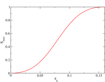
Figure 3: Graph of the maximum skewness parameter $S$ as defined in (32) as a function of $\epsilon_{g}$ for the grid given by (23b).

$\boldsymbol{N_{\xi}}$	$\boldsymbol{\epsilon_{g}=0.025}$	$\boldsymbol{\epsilon_{g}=0.05}$	$\boldsymbol{\epsilon_{g}=0.075}$	$\boldsymbol{\epsilon_{g}=0.15}$
16	2.08019E-3	3.27156E-3	5.57519E-3	8.99093E-3
32	5.07340E-4	8.20596E-4	1.44430E-3	2.34622E-3
64	1.25103E-4	2.03916E-4	3.62134E-4	5.90944E-4
128	3.10476E-5	5.07074E-5	9.02599E-5	1.47505E-4
256	7.73260E-6	1.26353E-5	2.25042E-5	3.67914E-5

Table 2: $L_{2}$-norm error between computational and analytic MMS potentials for different grid resolutions and grid nonuniformities ($\epsilon_{g}$) for the 2D nonorthogonal grid given by (23b). For these tests, we have again chosen $N_{\xi}=N_{\eta}$.

Turning our attention to the nonorthogonal grid (23b), we must now also consider the amount of “skewness” of the grid as a major factor in the difficulty associated with solving the curvilinear Poisson equation (26). In an effort to characterize the amount of nonorthogonality, or “skewness,” of our grids, we can use the Cauchy-Schwartz inequality [24], which states that any two points $\vec{p}$ and $\vec{q}$ in $n$-space must satisfy $\vec{p}\cdot\vec{q}\leq|\vec{p}||\vec{q}|$. Writing the contravariant metric tensor in the form $g^{\alpha\beta}(\vec{x}\,)=\nabla{\xi}^{\alpha}\cdot\nabla{\xi}^{\beta}$, the inequality can then be rewritten as

$$\nabla\xi\cdot\nabla\eta\leq|\nabla\xi||\nabla\eta|.$$ (31)

Squaring both sides and rearranging allows us to define the local grid skewness factor

$$S(\xi,\eta)=\frac{(\nabla\xi\cdot\nabla\eta)^{2}}{\left|\nabla\xi\right|^{2}\left|\nabla\eta\right|^{2}}=\frac{(g^{12})^{2}}{g^{11}g^{22}},$$ (32)

where $0\leq S\leq 1$. In the limit of $S(\xi,\eta)\rightarrow 0$, the grid is orthogonal at $(\xi,\eta)$, whereas for $S(\xi,\eta)\rightarrow 1$, the grid becomes singular, i.e. the grid cells become elongated and can fold. Furthermore, we can define the maximum grid skewness,

$$S_{\mathrm{max}}=\max\limits_{i,j}{\left[S(\xi_{i},\eta_{j})\right]},$$ (33)

as a single parameter to characterize the maximum nonorthogonality of the generated grid. Figure 3 shows $S_{\mathrm{max}}$ as a function of $\epsilon_{g}$ for the grid given by (23b). For $\epsilon_{g}\geq 0.125$, $S_{\mathrm{max}}$ is very nearly unity, and thus the grid is almost singular at some point on the grid. As noted above, this grid folds at $\epsilon_{g}=\frac{1}{2\pi}\approx 0.16$. As $S_{\mathrm{max}}\rightarrow 1$, the stiffness of the Laplacian matrix becomes quite large and the field solver will not easily converge, if at all.

The MMS tests performed on the nonorthogonal grid used the same MMS potential as was used for the orthogonal square grid (and again $f=1$). Table 2 shows that the $L_{2}$-norm of the error scales with second-order accuracy in $\Delta\xi=\Delta\eta$, as expected. We note here that the ratio of maximum cell area to minimum for the grid defined in (23b) scales according to $\frac{J_{max}}{J_{min}}=\frac{1+2\pi\epsilon_{g}}{1-2\pi\epsilon_{g}}$ ($\sim 34$ for $\epsilon_{g}=0.15$), meaning that the ratio of the largest cell area to the smallest is much smaller than that of the orthogonal, nonuniform grid case, but the skewness of the grid adds to the challenge and leads to errors comparable to those in Table 1.

We have also designed an MMS test to validate our Poisson solver for the annular grid generated in Section 2. We simulate half the annulus and apply symmetry conditions at the bottom. We apply either Dirichlet or Neumann boundary conditions along the inner and outer boundary segments, and symmetry requires homogenous Neumann boundary conditions along $\theta=0,\pi$. If the boundary conditions consist of only Neumann and periodic segments and no Dirichlet segments, the range of the Laplacian operator consists of densities that have total charge exactly equal to zero. Furthermore, this corresponds to a null space in the Laplacian operator $\Phi\rightarrow\Phi+\mathrm{const}.$ We have found that if we assure that the total charge is equal to zero, then the conjugate gradient algorithm converges quickly. The additional constant potential does not affect the electric field. We have therefore constructed the following potential:

$$\Phi\left(r,\theta\right)=1-r^{3}+\left(r-r_{1}\right)\left(r_{2}-r\right)\cos\theta,$$ (34)

where we have used polar coordinates to express (34) in the physical space, as it more naturally aligns with the annular grid case than the Cartesian notation we have been using until this point. At this point we should mention

As our Poisson solver is designed to solve general geometries in the physical space, we have applied the MMS test to both the azimuthally symmetric and axisymmetric cases ($f=1$ and $f=r$, respectively.) The physical Laplacian in this geometry with $f=1$, a cylindrical annulus, is given by (20a), leading to the physical charge density

$$\rho^{x}\left(r,\theta\right)=\frac{1}{4\pi}\left[9\,r+\left(3-\frac{r_{1}r_{2}}{r^{2}}\right)\cos\theta\right].$$ (35)

This density is then multiplied by the Jacobian and inserted into the Poisson solver with the proper boundary conditions.

$\boldsymbol{N_{\xi}}$	$\boldsymbol{R=5}$	$\boldsymbol{R=10}$	$\boldsymbol{R=20}$
16	4.86684E-3	8.78720E-3	1.35298E-2
32	1.18612E-3	2.15682E-3	3.35229E-3
64	2.92357E-4	5.32567E-4	8.29718E-4
128	7.25471E-5	1.32213E-4	2.06105E-4
256	1.80677E-5	3.29310E-5	5.13433E-5

(a) Cylindrical Laplacian

$\boldsymbol{N_{\xi}}$	$\boldsymbol{R=5}$	$\boldsymbol{R=10}$	$\boldsymbol{R=20}$
16	3.84324E-3	6.41377E-3	9.23903E-003
32	9.43887E-4	1.60080E-3	2.35531E-003
64	2.33099E-4	3.96923E-4	5.87121E-004
128	5.78702E-5	9.86410E-5	1.46102E-004
256	1.44142E-5	2.45755E-5	3.64121E-005

(b) Spherical Laplacian

Table 3: $L_{2}$-norm error between computational and analytic MMS potentials for different grid resolutions and ratios $R\equiv r_{2}/r_{1}$ for the annular grids generated in Section 2 for both Cartesian (a) and cylindrical (b) solvers. For these tests, we have again chosen $N_{\xi}=N_{\eta}$

In the axisymmetric system ($f=r$), the spherical radius satisfies $r_{s}^{2}=r^{2}+z^{2}$. The physical domain consists of an outer sphere of radius $r_{s2}$ is created in which an inner sphere of radius $r_{s1}$ has been removed. The corresponding physical charge density is obtained via (20b),

$$\rho^{x}\left(r_{s},\theta\right)=\frac{1}{4\pi}\left[12\,r_{s}+\left(4-\frac{2r_{s1}r_{s2}}{r_{s}^{2}}\right)\cos\theta\right].$$ (36)

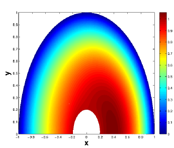
(a)

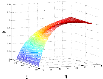
(b)

Figure 4: Two-dimensional MMS potential plots as obtained computationally using (35) and (36) in physical (a) and logical (b) space.

The $L_{2}$-norm of the error for both azimuthal and axisymmetric solvers is shown in Table 3. Here $R=r_{2}/r_{1}$ $\left(\mathrm{or}\,r_{s2}/r_{s1}\right)$ is the ratio of the radius of the outer boundary to that of the inner boundary and $N_{\xi,\eta}$ is the number of uniformly spaced grid points in each direction. Figure 4 displays the chosen MMS potential on both the physical and logical domains as obtained by the logical grid Poisson solver. Notice that the different values of $\rho^{\xi}$ inserted in the solver for the different coordinate systems should (and do) return the same potential on the grid. The results shown in Tables 2 and 3 show the expected second-order scaling with grid spacing, showing that our field solver is working correctly.

6.3 Self-Fields and Momentum Conservation

With a uniform grid, symmetrical particle shapes guarantee exact momentum conservation if the gridding is done correctly [3]. For a uniform rectangular grid, this is equivalent to having the self-electric forces exactly zero on each particle. (24b) dictates that we use the logical grid electric field at the particle’s position on the logical grid. The most obvious method to do this is by simply differencing $\Phi$ with respect to $\xi$, (where we have defined a staggered mesh such that $E^{\xi}$ exists on vertices and $\Phi$ and $\rho^{\xi}$ exist on cell centers). One then interpolates $E^{\xi}$ to the logical space particle position. Unfortunately, simple 1d tests on this method of obtaining the logical electric field with a single particle reveal a non-zero self-field at the particle.

We have therefore devised a second, less direct method of obtaining the logical electric fields at the particle position in which we solve for the electric field on the logical grid and interpolate this field to the particle position. As such, we calculate the electric field on the vertices, formulated on the logical grid as

$$E^{\xi}_{i,j}=-\frac{\Phi_{i+\frac{1}{2},j+\frac{1}{2}}-\Phi_{i-\frac{1}{2},j+\frac{1}{2}}+\Phi_{i+\frac{1}{2},j-\frac{1}{2}}-\Phi_{i-\frac{1}{2},j-\frac{1}{2}}}{2\Delta\xi}$$ (37a)

and

$$E^{\eta}_{i,j}=-\frac{\Phi_{i+\frac{1}{2},j+\frac{1}{2}}-\Phi_{i+\frac{1}{2},j-\frac{1}{2}}+\Phi_{i-\frac{1}{2},j+\frac{1}{2}}-\Phi_{i-\frac{1}{2},j-\frac{1}{2}}}{2\Delta\eta}.$$ (37b)

We then apply the proper extrapolation techniques such that the overall second-order accuracy of the system is upheld and calculate the physical electric fields on the vertices using

$$E^{x}_{i,j}=\frac{1}{J^{v}_{i,j}}\left(j^{v}_{22,i,j}E^{\xi}_{i,j}-j^{v}_{21,i,j}E^{\eta}_{i,j}\right)$$ (38a)

and

$$E^{y}_{i,j}=\frac{1}{J^{v}_{i,j}}\left(j^{v}_{11,i,j}E^{\eta}_{i,j}-j^{v}_{12,i,j}E^{\xi}_{i,j}\right),$$ (38b)

where we have transformed from the inverse Jacobian matrix, $k^{\mu\nu}$ to the Jacobian matrix $j_{\mu\nu}$. Here, the superscript $v$ on the components of the Jacobi matrix and its determinant signify that they are calculated on the vertices using a four-point average from their natural cell-centered locations. This technique for calculating the electric fields at the particles leads to exactly zero self-forces on a test particle in 1d, but in 2d the Jacobi matrix components do not exactly cancel, leading to non-zero self-forces on the particles. Reference [17] provides a detailed explanation as to why this method leads to non-zero self-forces at the particle and a detailed comparison of this method with the direct interpolation method detailed above. We stress that, with a non-uniform grid, zero self-forces do not guarantee exact momentum conservation because of the presence of the inertial terms in (14), which are often larger than the self-force terms [17].

6.3.1 Logical Electric Fields at a Particle

To test the self-forces on the particle in 2d, we have set up a system in which a single particle is at rest on a doubly-periodic grid with a neutralizing background such that we can interpolate both of the physical electric fields and required grid derivatives to the grid positions and retroactively multiply them to obtain the logical fields at the particle position. As mentioned above, we expect to have some small self-force in 2d by utilizing this method. Below we attempt to quantify these forces.

In 2d, the logical electric fields are obtained from the physical fields using

$$\frac{\partial\Phi}{\partial\xi^{\mu}}=\frac{\partial x^{\nu}}{\partial\xi^{\mu}}\frac{\partial\Phi}{\partial x^{\nu}}$$ (39)

such that

$$\begin{array}[]{rcl}E^{\xi}&=&j_{11}\,E^{x}+j_{21}\,E^{y}\\ E^{\eta}&=&j_{12}\,E^{x}+j_{22}\,E^{y}.\end{array}$$ (40)

For a uniform grid, the electric fields at the particle are zero to machine precision. However, as soon as we allow one of the grid dimensions to become nonuniform, the fields at the particle in the nonuniform dimension are no longer zero, even for $\epsilon_{g}=10^{-4}$. We find that the fields at the particle position scale with second-order accuracy in grid spacing, and the magnitude of the field at the particle in the nonuniform dimension is dependent upon the magnitude of the grid nonuniformity parameter, $\epsilon_{g}$. For example, using a grid with $N_{\xi}=N_{\eta}=32$ where $\epsilon_{g}=0.15$ in $x$ and holding $y$ to be uniform ($\epsilon_{g}=0$), $E^{\xi}(\xi_{p},\eta_{p})\approx 10^{-5}$, whereas $E^{\eta}(\xi_{p},\eta_{p})$ is zero to machine precision. For $\epsilon_{g}=0.1$, $E^{\xi}(\xi_{p},\eta_{p})\approx 10^{-7}$ for the same grid resolution.

We have also tried the direct interpolation method, i.e. directly interpolating the logical electric field $E^{\xi}$ on the logical grid to the particle position. This method also scales with second-order accuracy in grid spacing, but the indirect method detailed above consistently provides smaller fields at the particle position.

7 NUMERICAL RESULTS

We have performed several benchmarking tests to validate the full 2D curvilinear coordinate PIC code. For all tests presented below, we use a nonuniformity parameter of $\epsilon_{g}=0.1$ (for both orthogonal and nonorthogonal grids). This leads to a ratio of areas of the largest cell to smallest of $\sim 20$ for the nonuniform orthogonal grid (23a) and $\sim 4.4$ for the nonorthogonal grid (23b). The maximum skewness parameter $S_{\mathrm{max}}$ is $\sim 0.75$ for the nonorthogonal grid with this nonuniformity parameter. We have done only high frequency tests and have accordingly assumed that the ions are an immobile background, providing charge neutrality in the equilibrium. We have normalized the equations so that the electron plasma frequency $\omega_{pe}$ is equal to unity.

7.1 Cold Plasma Oscillations on a Square Physical Domain

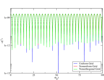
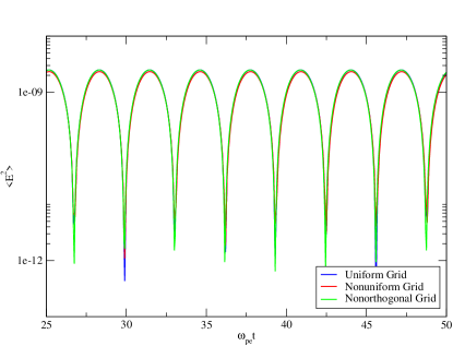
Figure 5: Comparison of cold plasma oscillation field energies using a uniform grid and the nonuniform grids given by (23a) and (23b) for (a) a long run and (b) a zoomed section of the run showing an oscillation period of $2\pi$ for all three grids. Here we have used quadratic $(S_{2})$ particle shape functions with $N_{\xi}=N_{\eta}=128$, $\bar{N}_{\mathrm{ppc}}=225$, $\Delta t=0.025$, and $\epsilon_{g}=0.1$ (for the nonuniform case).

Figure 5 shows a comparison of the evolution of the electrostatic field energy, defined in 2d as

$$<E^{2}>=\frac{1}{2}\int dx\,dy\left[(E^{x})^{2}+(E^{y})^{2}\right],$$ (41)

for a cold plasma oscillation on the uniform, nonuniform but orthogonal, and nonorthogonal grids. For these tests, we take a cold distribution of electrons with a uniform density stationary ion background and initialize a perturbation in the system by perturbing the particle positions with respect to the uniform neutralizing background. We define the quantity $\epsilon_{\mathrm{pert}}$ to be the size of this initial perturbation on the particle positions. The initial particle positions, whether assigned uniformly in the physical space or assigned according to the Jacobian in the logical space, lead to a perturbed charge density. This perturbation can dominate $\epsilon_{\mathrm{pert}}$ if the latter is small enough. For these tests, the initial particle perturbation is directed at a $45^{\circ}$ angle across the grid to check the effects of the interpolation in multiple dimensions on the data produced. In Figure 5, we show both a long-time evolution and a zoomed section of the field energy from these same runs. We have used a perturbation of $\vec{\epsilon}_{\mathrm{pert}}=(7.07e^{-5},7.07e^{-5})$, such that the magnitude of the perturbation is $|\vec{\epsilon}_{\mathrm{pert}}|=1\times 10^{-4}$, $N_{\xi}=N_{\eta}=128$, the average number of particles per cell is $\bar{N}_{\mathrm{ppc}}=225$, and $\omega_{pe}\Delta t=0.025$. No measurable growth in the electrostatic field energy was observed during the course of these runs. We note that the period of the plasma oscillations observed in Figure 5 is very nearly $2\pi$ (as is expected for $\omega_{pe}=1$) for all three grid choices. Further testing has revealed that the period of the plasma oscillations converges to the value of $2\pi$ with second-order accuracy in $\Delta t$, as expected, and the electric field energy does not begin to decay even in very long runs.

7.2 Cold Electron-Electron Two-Stream Instability

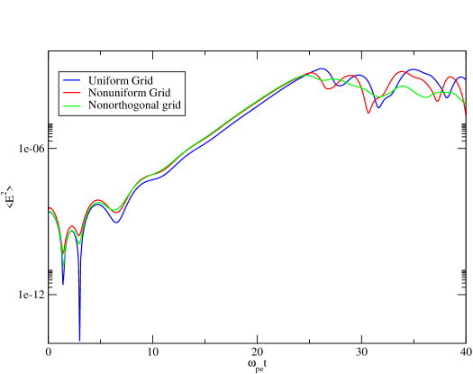
Figure 6: Comparison of cold electron-electron two-stream instability growth rates for uniform and non-uniform grids. Higher initial noise levels due in the nonuniform grid case provide a larger initial perturbation in the system, leading to the differences seen between the two curves. Here we have used quadratic particle shape functions with $N_{\xi}=N_{\eta}=128$, $\bar{N}_{\mathrm{ppc}}=225$, $\Delta t=0.025$ for all cases, with $\epsilon_{g}=0.1$ for the nonuniform orthogonal and nonorthogonal cases.

Having chosen a physical grid such that $x,y\in[-\pi:\pi]$, the wave vector $\vec{k}$ is given by $\vec{k}=[1,1]$, such that, to generate a two stream instability at a $45^{\circ}$ degree angle across the grid, we use the effective wave vector, $k^{45^{\circ}}=\sqrt{2}\approx 1.414$. In our normalized units, the maximum growth rate for the two stream instability of $\sim 0.35$ occurs at $|\vec{k}\cdot\vec{v}_{0}|\approx 0.63$. As such, we have chosen an initial velocity parallel to $\vec{k}$ (in the physical space) with $\vec{v}=[0.314,0.314]$.

Figure 6 shows the time evolution of the electrostatic field energy for a uniform grid compared with the nonuniform grids given by (23a) and (23b). The offset of the three curves is due to the larger initial perturbation due to the grid non-uniformity discussed above. Here we have used quadratic particle shape functions with $N_{\xi}=N_{\eta}=128$, $\bar{N}_{\mathrm{ppc}}=225$, $\omega_{pe}\Delta t=0.025$ for all cases, again with $\epsilon_{g}=0.1$ for the nonuniform orthogonal and nonorthogonal cases. The same cases have been performed using bilinear particle shape functions, revealing identical results. For all cases, the observed growth rate is $\sim 0.35$, which matches the theoretical prediction.

7.3 Landau Damping

In this section we study the effects of Landau damping with our 2D code, on a unit square physical grid. Since the our thermal distribution is taken to be Maxwellian, the particle velocities are isotropic in $x,y$, and as such we have set up a case in which the initial perturbation is only in $x$ for simplicity. Figure LABEL:Fig:2d_LD_GR_comp shows the time evolution of the Landau damping on our electrostatic field energy for the uniform, nonuniform orthogonal and nonorthogonal square grids. Here we have used $N_{\xi}=N_{\eta}=128$, $\bar{N}_{\mathrm{ppc}}=400$, $\Delta t=0.025$, and $v_{th}=0.07$ for all cases. Note that the nonorthogonal grid more closely follows the damping rate of the uniform grid than does the nonuniform, orthogonal grid. The real oscillation frequency agrees very well with the theoretical value of $0.58$ given by the Bohm-Gross dispersion relation [25] $\omega^{2}=\omega_{pe}^{2}+3k^{2}v_{th}^{2}$, where again we have taken $\omega_{pe}=1$ in accordance with our code normalizations. The average damping rate across the simulation time agrees to within $3\%$ of the theoretical value of $0.124$ as given by [25]

$$\omega_{i}=-\sqrt{\frac{\pi}{8}}\frac{\omega_{pe}}{|k^{3}\lambda_{De}^{3}|}\exp{\left[-\left(\frac{1}{2k^{2}\lambda_{De}^{2}}+\frac{3}{2}\right)\right]}$$ (42)

for these parameters for the uniform and nonorthogonal grids, whereas the damping rate on nonuniform, orthogonal grid agrees to within $5\%$. We hypothesize that the lower damping rate observed for the nonuniform orthogonal grid case (23b) is due to the strong nonuniformity of the grid; the ratio of the largest to the smallest cell areas for a nonuniformity parameter $\epsilon_{g}=0.1$ is $\sim 20$. To check this hypothesis, we have also run cases in which we have used $\epsilon_{g}=0.06$ such that the largest to smallest cell area ratio is $\sim 4.9$. These cases give the same damping rates as the uniform grid case shown above.

7.4 Cold Plasma Oscillations on a Concentric Annulus

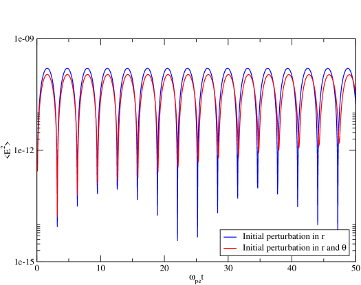
Figure 7: Comparison of cold plasma oscillation field energies on an annular physical grid using an initial perturbation in $r$ only and a combination of $r$ and $\theta$ initial perturbation showing an oscillation period very close to $2\pi$ for both cases. Here we have used quadratic spline particle shape functions with $N_{\xi}=N_{\eta}=64$, $\bar{N}_{\mathrm{ppc}}=400$, and $\Delta t=0.05$.

As a final test of our entire method, we have set up a cold plasma oscillation on the concentric annulus grid of Figure 2a (taking azimuthal symmetry). As an initial test, we perturbed the initial potential radially using

$$\tilde{\Phi}=\epsilon_{\mathrm{pert}}\cos{\left(\pi\left(\frac{r-r_{1}}{r_{2}-r_{1}}\right)\right)},$$ (43)

where we have used $\epsilon_{\mathrm{pert}}=10^{-4}$, $r_{1}=0.25$, and $r_{2}=1.0$. This initial perturbation satisfies homogeneous Neumann boundary conditions along the entire boundary of the system.

In general, for Neumann boundary conditions, there is a subtlety, namely that the unit normal to the physical dommain does not map to the unit normal in the logical domain. Thus, Neumann boundary conditions involve the normal and tangential derivatives on the logical boundary. For this case, however, the Winslow coordinates are orthogonal, and this issue does not arise. See Sec. 6.2 for a discussion of the associated null space issues.

With our input parameters, the ratio of the area of the largest grid cell to the smallest is $\sim 16.$ This is a very simple test of the system, and is analogous to perturbing our system only in $y$ on a rectangular grid. The time evolution of the electrostatic field energy for this test is shown in the blue curve of Figure 7 for a $64\times 64$ physical grid with $\omega_{pe}\Delta t=0.1$, $\bar{N}_{\mathrm{ppc}}=225$, and quadratic spline shape functions. The period of oscillation of the field energy for this set of initial conditions is observed to be $\sim 6.3$ for this case, meaning that the frequency is indeed unity with an error that scales as $\Delta\xi^{2}$, as per our code normalizations.

As a more challenging case, we then perturbed the initial potential using

$$\tilde{\Phi}=\epsilon_{\mathrm{pert}}\cos{\left(\pi\left(\frac{r-r_{1}}{r_{2}-r_{1}}\right)\right)}\cos\theta,$$ (44)

where we have again used $\epsilon_{\mathrm{pert}}=10^{-4}$, $r_{1}=0.25$, and $r_{2}=1.0$. The red curve in Figure 5 shows the time evolution of the electrostatic field energy for a $64\times 64$ physical grid with $\omega_{pe}\Delta t=0.05$, $\bar{N}_{\mathrm{ppc}}=400$, and quadratic spline shape functions. We have used more resolution in this particular case in order to resolve more fully the complicated features of our initial potential. Again, the measured period of oscillation is $\sim 6.3$ (the difference between the two curves is approximately $0.085\%$); giving frequency unity, with errors scaling as $\Delta\xi^{2}$.

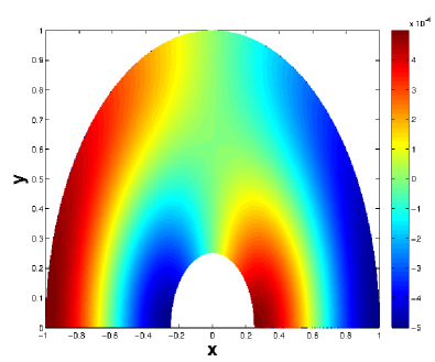
(a) $\omega_{pe}\,t=1.6$

(b) $\omega_{pe}\,t=2.8$

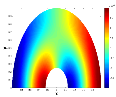
(c) $\omega_{pe}\,t=3.6$

(d) $\omega_{pe}\,t=4.8$

Figure 8: Snapshots of one period of the evolution the potential of a cold plasma oscillation on the annular physical grid. Here we have perturbed the inital potential using (44).

Figure 8 shows the time evolution of one period of the potential on the physical grid using the initial perturbation as given by (44) for the cold electrostatic plasma oscillation test described above. Figures 8(a) and (b) are from one half of the plasma period and Figures 8(c) and (d) are from the next. Notice the exact reversal of the potentials between the two halves of the plasma period. Reflecting boundary conditions for particles at the non-periodic parts of the boundary were not required for this case, because the particle excursions for a cold plasma oscillation are so small.

8 CONCLUSIONS

In this study, we have set out to develop a new approach to the PIC method, in which the key components, the mover, the field solve, charge accumulation, and field interpolation, are carried out on a uniform grid in the logical domain, the unit square, and mapped to an arbitrary boundary conforming grid on an arbitrary physical domain. We have focused on a 2d, electrostatic model as a proof of principle.

To demonstrate our method, we used analytically prescribed grids and grids obtained by Winslow’s grid generation technique [15] to generate a boundary-fitted grid, in the latter case by solving a set of coupled elliptic equations using a nonlinear Newton-Krylov solver. The generated grids are then mapped onto the logical grid through the use of the mapping $\vec{x}(\vec{\xi}\,)$ and its inverse, $\vec{\xi}(\vec{x})$, such that the PIC components can be run on the logical grid using these mappings.

We have derived the logical grid macroparticle equations of motion based on a canonical transformation of Hamilton’s equations from the physical domain to the logical. The resulting nonseparable system of equations using an extended form of the semi-implicit modified leapfrog integrator [21], which we have shown to be symplectic for a system of arbitrary dimension and second-order accurate in time if symmetrization leading to a time-centered discretization of the macroparticle update equations is utilized. If the field solve is performed just after the first step of this integrator, it needs to be done only once per time step.

In order to obtain the electrostatic fields on the logical grid, we have constructed a generalized curvilinear coordinate formulation of Poisson’s equation which is discretized conservatively on the logical grid using a staggered mesh. Field boundary conditions are applied in such a way as to produce a symmetric operator matrix which we then solve using a conjugate gradient solver.

Our formulation of the curvilinear coordinate Poisson equation requires the logical grid charge density, which allows us to accumulate the charge from the particles directly onto the uniform, square logical grid using standard particle shape functions rather than the more complicated, weighted shape functions which must be used if the charge is accumulated on a nonuniform physical grid. Furthermore, the particle equations of motion require that the derivative of the electrostatic potential on the logical grid be obtained at the particle positions for the update of the particle momentum. These logical electric fields are interpolated to the particle positions on the logical grid using the symmetric particle shape functions which have been slightly modified from the standard shape functions used in the charge accumulation process in order to account for our choice of a staggered mesh. All validation tests performed have shown that the code produces correctly the physics for complicated interior meshing, as well as for complicated domain shapes.

Albeit at a proof-of-principle level, our code has shown that an arbitrary coordinate PIC method is a an accurate and efficient alternative to current methods for simulating plasma systems with complex domains. Future work will focus on extending the method to 3d and extending to electromagnetic systems. Further, work is required on parallelization techniques to handle more efficiently the particle push and charge accumulation stages of our method. Finally, our method can be coupled to a moving mesh algorithm to more accurately follow the dynamic evolution of the plasma system.

Appendix A Differential Geometry Notation

This Appendix presents the reader with a coherent overview of the relations between Cartesian and curvilinear coordinates which form the basis of this paper.

Let the values $x^{\alpha},\alpha=1,\cdots,n$ be the Cartesian coordinates of the vector ${\vec{x}}$. The coordinate transformation ${\vec{x}}(\vec{\xi}\,)$ defines a set of curvilinear coordinates $\xi^{\alpha},\cdots,\xi^{n}$ in the domain $X^{n}$. We define the Jacobi matrix of this transformation

$$j_{\alpha\beta}(\vec{\xi}\,)\equiv\left(\frac{\partial x^{\alpha}}{\partial\xi^{\beta}}\right),\quad\alpha,\beta=1,\cdots,n,$$ (45)

and its Jacobian

$$J(\vec{\xi\,})\equiv\mbox{det}\left(\boldsymbol{j}\right).$$ (46)

Conversely, we can also think of this transformation as a mapping of $\vec{\xi}$ to $\vec{x}$, $\vec{\xi}(\vec{x}\,)$. Defining the inverse of the matrix $j_{\alpha\beta}$ as

$$k^{\alpha\beta}(\vec{x}\,)\equiv\left(\frac{\partial\xi^{\alpha}}{\partial x^{\beta}}\right),\quad\alpha,\beta=1,\cdots,n,$$ (47)

we can write its Jacobian

$$K(\vec{x})\equiv\mbox{det}\left(\boldsymbol{k}\right)=\frac{1}{J}.$$ (48)

Simple linear algebra tells us that

$$j_{\alpha\beta}k^{\beta\gamma}=\frac{\partial x^{\alpha}}{\partial\xi^{\beta}}\frac{\partial\xi^{\beta}}{\partial x^{\gamma}}\equiv\delta_{\alpha}^{\gamma},$$ (49)

therefore $\boldsymbol{j}\boldsymbol{k}=\boldsymbol{I}$.

Given a Euclidean metric on the physical space, we have

$$dx^{\gamma}dx^{\gamma}=\frac{\partial x^{\gamma}}{\partial\xi^{\alpha}}\frac{\partial x^{\gamma}}{\partial\xi^{\beta}}d\xi^{\alpha}d\xi^{\beta}=g_{\alpha\beta}d\xi^{\alpha}d\xi^{\beta},$$ (50)

and the covariant metric tensor is defined as

$$g_{\alpha\beta}(\vec{\xi}\,)\equiv\frac{\partial x^{\gamma}}{\partial\xi^{\alpha}}\frac{\partial x^{\gamma}}{\partial\xi^{\beta}},\quad\alpha,\beta,\gamma=1,\cdots,n.$$ (51)

From (45), we see $g_{\alpha\beta}=j_{\gamma\alpha}j_{\gamma\beta}$, which is simply $\boldsymbol{g}_{\mathrm{cov}}=\boldsymbol{j}^{T}\boldsymbol{j}$. Likewise, the contravariant metric tensor is based upon the inverse Jacobian matrix, $\boldsymbol{k}$:

$$g^{\alpha\beta}(\vec{x}\,)\equiv\frac{\partial\xi^{\alpha}}{\partial x^{\gamma}}\frac{\partial\xi^{\beta}}{\partial x^{\gamma}},\quad\alpha,\beta,\gamma=1,\cdots,n,$$ (52)

thus $\boldsymbol{g}^{\mathrm{con}}=\boldsymbol{k}\boldsymbol{k}^{T}$.

Finally, by multiplying the covariant and contravariant metric tensors and applying the identity $\boldsymbol{j}\boldsymbol{k}=\boldsymbol{I}$, we can prove that the covariant and contravariant metric tensors are in fact inverses of each other:

$$\boldsymbol{g}_{\mathrm{cov}}\boldsymbol{g}^{\mathrm{con}}=\boldsymbol{j}^{T}\boldsymbol{j}\boldsymbol{k}\boldsymbol{k}^{T}=\boldsymbol{j}^{T}\boldsymbol{k}^{T}=\left(\boldsymbol{k}\boldsymbol{j}\right)^{T}=\boldsymbol{I}^{T}=\boldsymbol{I}.$$ (53)

In two dimensions, we can easily convert from the covariant to the contravariant metric tensor using the following equation:

$$g^{\alpha\beta}=\left(-1\right)^{\alpha+\beta}\frac{g_{3-\alpha,3-\beta}}{g_{\mathrm{cov}}},\quad\alpha,\beta=1,2,$$ (54)

where $g_{\mathrm{cov}}=J^{2}$ is the determinant of the covariant metric tensor, and $g_{\mathrm{cov}}=\frac{1}{g^{\mathrm{con}}}$, where $g^{\mathrm{con}}=K^{2}$ is the determinant of the contravariant metric tensor. Likewise, we can shift from the contravariant to the covariant metric tensor using

$$g_{\alpha\beta}=\left(-1\right)^{\alpha+\beta}g_{\mathrm{cov}}g^{3-\alpha,3-\beta},\quad\alpha,\beta=1,2.$$ (55)

Appendix B Derivation of Curvilinear Coordinate Poisson Equation

We begin by rewriting (3) as the divergence of the gradient of the potential in generalized coordinates:

$$\frac{1}{f}\nabla\cdot f\nabla\Phi=\frac{1}{f}\frac{\partial}{\partial x^{\alpha}}\cdot f\frac{\partial\Phi}{\partial x^{\alpha}}=-4\pi\rho,$$ (56)

where $f$ is a geometry factor allowing us to switch between azimuthal and axially-symmetric systems. For instance, if we want the physical coordinate system to be $x,y$ with $\frac{\partial}{\partial z}=0$, we set $\mathit{f}=1$. For $r,z$ coordinates with $\frac{\partial}{\partial\phi}=0$, we set $\mathit{f}=r.$

In matrix notation we can write $\nabla\Phi$ as

$$\nabla\Phi = \frac{\partial{\Phi}}{\partial{\xi^{m}}}\nabla\xi^{m}$$ (57)

$$= A_{m}\nabla\xi^{m}$$

where $A_{m}$ are the covariant components of the 2D vector

$$\vec{A}=A_{m}\nabla\xi^{m}=A_{1}\nabla\xi+A_{2}\nabla\eta.$$ (58)

Likewise, we can represent $\vec{A}$ by its contravariant components, $A^{m}$:

$$\vec{A}=A^{1}\nabla\eta\times\hat{z}+A^{2}\hat{z}\times\nabla\xi,$$ (59)

such that we can write

$$A_{1}\nabla\xi+A_{2}\nabla\eta=A^{1}\nabla\eta\times\hat{z}+A^{2}\hat{z}\times\nabla\xi.$$ (60)

We can now find the direct relationship between the covariant and contravariant components of $\vec{A}$. For example, taking the inner product of (60) with $\nabla\eta\times\hat{z}$ we find:

$$A^{1}\left(\nabla\eta\times\hat{z}\right)\cdot\nabla\xi=A_{1}|\nabla\xi|^{2}+A_{2}\nabla\eta\cdot\nabla\xi.$$ (61)

By (52),

$$\nabla\xi^{\beta}\cdot\nabla\xi^{\gamma}=g^{\beta\gamma},$$ (62)

allowing us to rewrite (61) as

$$A_{1}g^{11}+A_{2}g^{12}=A^{1}\left(\nabla\eta\times\hat{z}\right)\cdot\nabla\xi=A^{1}\nabla\xi\cdot\nabla\eta\times\hat{z}.$$ (63)

We note that

$$\nabla\xi\cdot\nabla\eta\times\hat{z} = \frac{\partial\xi}{\partial x}\frac{\partial\eta}{\partial y}-\frac{\partial\xi}{\partial y}\frac{\partial\eta}{\partial x}$$ (64)

$$= \det{(\boldsymbol{k})}$$

$$= \frac{1}{J},$$

so we can write the left-hand side of (63) as

$$A_{1}g^{11}+A_{2}g^{12}=\frac{A^{1}}{J}.$$ (65a)

Similarly,

$$A_{1}g^{21}+A_{2}g^{22}=\frac{A^{2}}{J}.$$ (65b)

Returning now to (56) and using (57) and (59) and the identity

$$\nabla\cdot(c\vec{v})=\nabla c\cdot\vec{v}+c\nabla\cdot\vec{v},$$ (66)

we can write the Laplacian operator as

$$\frac{1}{f}\nabla\cdot f\nabla\Phi = \nabla\cdot\vec{A}$$

$$= \frac{1}{f}\nabla\cdot\left[fA^{1}(\nabla\eta\times\hat{z})+fA^{2}(\hat{z}\times\nabla\xi)\right]$$

$$= \frac{1}{f}\left[\nabla(fA^{1})\cdot(\nabla\eta\times\hat{z})+\nabla(fA^{2})\cdot(\hat{z}\times\nabla\xi)\right].$$

Using $\nabla\xi\cdot(\nabla\xi\times\hat{z})=0$, (B) can be written as

$$\frac{1}{f}\nabla\cdot f\nabla\Phi=\left[\frac{1}{f}\frac{\partial(fA^{1})}{\partial\xi}\nabla\xi\cdot(\nabla\eta\times\hat{z})+\frac{1}{f}\frac{\partial(fA^{2})}{\partial\eta}\nabla\eta\cdot(\hat{z}\times\nabla\xi)\right].$$ (67)

By (64), we can rewrite (67) as

$$\frac{1}{f}\nabla\cdot f\nabla\Phi=\frac{1}{fJ}\left(\frac{\partial(fA^{1})}{\partial\xi}+\frac{\partial(fA^{2})}{\partial\eta}\right)=-\frac{\rho}{\epsilon_{0}}.$$ (68)

Now converting the contravariant components of $\vec{A}$ to their covariant formulations using (57) and (63), we can write the final form of the Poisson equation in curvilinear coordinates:

$$\frac{1}{fJ}\frac{\partial}{\partial\xi^{\alpha}}\left(fJg^{\alpha\beta}\frac{\partial\Phi}{\partial\xi^{\beta}}\right)=-4\pi\rho,$$ (69)

where $\rho=\rho^{x}$ is the physical charge density.

References

References

- [1] D. R. Nicholson. Introduction to Plasma Theory. Kreiger Publishing Company, 1992.
- [2] G. F. Carrier and C. E. Pearson. Partial Differential Equations: Theory and Technique. Academic Press, Boston, 1988.
- [3] C. K. Birdsall and A. B. Langdon. Plasma Physics via Computer Simulation. Adam Hilger, New York, 1991.
- [4] J. M. Dawson. Particle simulation of plasmas. Reviews of Modern Physics, 55:403, 1983.
- [5] M. E. Jones. Electromagnetic PIC codes with body-fitted coordinates. International Conference on the Numerical Simulation of Plasmas, 1987. (San Francisco, CA), Talk IM3.
- [6] T. Westermann. Electromagnetic Particle-in-Cell simulations of the self-magnetically insulated -diode. Nuclear Instruments and Methods in Physics Research, A281:253, 1989.
- [7] C.-D. Munz, R. Schneider, E. Sonnendrücker, E. Stein, U. Voss, and T. Westermann. A finite-volume Particle-in-Cell method for the numerical treatment of Maxwell-Lorentz equations on boundary-fitted meshes. International Journal for Numerical Methods in Engineering, 44:461, 1999.
- [8] J. W. Eastwood, W. Arter, N. J. Brealey, and R. W. Hockney. Body fitted electromagnetic PIC software for use on parallel computers. Computer Physics Communications, 87:155, 1995.
- [9] T. Westermann. Particle-in-Cell simulations with moving boundaries – Adaptive mesh generation. Journal of Computational Physics, 114:161, 1994.
- [10] G. Lapenta. Automatic adaptive multi-dimensional Particle-in-Cell. Advanced Methods for Space Simulations, page 61, 2007.
- [11] D. Seldner and T. Westermann. Algorithms for interpolation and localization in irregular 2d meshes. Journal of Computational Physics, 79:1, 1988.
- [12] T. Westermann. Localization schemes in 2d boundary-fitted grids. Journal of Computational Physics, 101:307, 1992.
- [13] G. L. Delzanno, L. Chacón, J. M. Finn, Y. Chung, and G. Lapenta. An optimal robust equidistribution method for two-dimensional grid generation based on Monge-Kantorovich optimization. Journal of Computational Physics, 227:9841, 2008.
- [14] D. R. Welch, T. C. Genoni, R. E. Clark, and D. V. Rose. Adaptive particle management in a paricle-in-cell code. Journal of Computational Physics, 227:143, 2007.
- [15] A. M. Winslow. Numerical solution of the quasilinear Poisson equation in a nonuniform triangle mesh. Journal of Computational Physics, 2:149, 1967.
- [16] V. D. Liseikin. Grid Generation Methods. Springer-Verlag, Berlin, Heidelberg, New York, 1999.
- [17] C. A. Fichtl. An Arbitrary Curvilinear Coordinate Particle In Cell Method. PhD thesis, University of New Mexico, 2010.
- [18] C. T. Kelley. Iterative Methods of Linear and Nonlinear Equations. SIAM, Philadelphia, 1995.
- [19] R. Dembo, S. Eisenstat, and R. Steihaug. Inexact Newton methods. Journal of Numerical Analysis, 19:400, 1982.
- [20] H. Goldstein. Classical Mechanics. Addison-Wesley, Massachusetts, 1965. p. 239-245.
- [21] J. M. Finn and L. Chacón. Volume preserving integrators for solenoidal fields on a grid. Physics of Plasmas, 12:054503, 2005.
- [22] L. Chacon. Private communication, June 2010.
- [23] P. J. Roache. Code verification by the method of manufactured solutions. Journal of Fluids Engineering, 127:4, 2002.
- [24] R. C. Buck. Advanced Calculus. McGraw-Hill Book Company, New York, 1965.
- [25] N. A. Krall and A. W. Trivelpiece. Principles of Plasma Physics. San Francisco Press, San Francisco, 1986.