Ultracold atom research presents many avenues to study problems at the forefront of physics. Due to their unprecedented controllability, these systems are ideally suited to explore new exotic states of matter, which is one of the key driving elements of the condensed matter research. One such topic of considerable importance is topological insulators, materials that are insulating in the interior but conduct along the edges. Quantum Hall and its close cousin Quantum Spin Hall states belong to the family of these exotic states and are the subject of this chapter.

Contents

• Ultracold atoms, synthetic gauge fields, and topological states ……… 1

• Topological aspects: Chern numbers and edge states………………………3

• The Hofstadter model and the Chern number………………………………….4

• Chern-Dimer mapping for anisotropic lattices……………………………….6

• Chern numbers in time of flight measurements……………………………..8

• Incommensurate flux: Chern tree……………………………………………..11

• Quantum spin-Hall effects with ultracold atoms…………………………15

• Open questions and outlooks………………………………………………….18

Ultracold Atoms, synthetic gauge fields, and topological states

Quantum engineering, i.e., preparation, control and detection of quantum systems, at micro- to nano-Kelvin temperatures has turned ultracold atoms into a versatile tool for discovering new phenomena and exploring new horizons in diverse branches of physics. Following the seminal experimental observation of Bose Einstein condensation, simulating many-body quantum phenomena using cold atoms, which in a limited sense realizes Feynman’s dream of quantum simulation, has emerged as an active frontier at the cross section of AMO and condensed matter physics. There is hope and excitement that these highly tailored and well controlled systems may solve some of the mysteries regarding strongly correlated electrons, and pave ways for the development of quantum computers.

The subject of this chapter is motivated by recent breakthroughs in creating “artificial gauge fields” that couple to neural atoms in an analogous way that electromagnetic fields couple to charged particles [1]. This opens up the possibility of studying quantum Hall (QH) states and its close cousin quantum spin Hall (QSH) states, which belong to the family of exotic states of matter known as Topological Insulators.

QH and QSH effect usually requires magnetic field and spin-orbit coupling, respectively. In contrast to electrons in solids, cold atoms are charge neutral and interact with external electromagnetic field primarily via atom-light coupling. Artificial orbital magnetic field can be achieved by rotating the gas [9]. In the rotating frame, the dynamics of atoms becomes equivalent to charged particles in a magnetic field which is proportional to the rotation frequency. To enter the quantum Hall regime using this approach requires exceedingly fast rotation, a task up to now remains a technical challenge. In this regard, another approach to engineer artificial magnetic field offers advantages. This involves engineering the (Berry’s) geometric phase of atoms by properly arranging inhomogeneous laser fields that modify the eigenstates (the dressed states) via atom-light coupling [10]. Such geometric phase can mimic for example the Aharonov-Bohm phase of orbital magnetic field. Because the dressed states can be manipulated on scales of the wavelength of light, the artificial gauge fields can be made very strong. For example, the phase acquired by going around the lattice unit cell can approach the order of $\pi$. This gives hope to enter the quantum Hall regime. The strength of this approach also lies in its versatility. Artificial gauge fields in a multitude of forms, either Abelian (including both electric and magnetic field) or non-Abelian (including effective spin-orbit coupling), can be introduced for continuum gases or atoms in optical lattices [10]. Recent NIST experiments have successfully demonstrated artificial magnetic field [1] as well as spin-orbit coupling [2] for bosonic Rb atoms and experiments are underway to reach QH and QSH regimes.

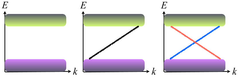
Figure 1: Figure illustrates distinction between ordinary band insulator (left), QH (middle) and QSH (right) insulators in the energy spectrum. Connecting the conduction and valence bands are the edge states.

Topological aspects: Chern numbers and edged states

Topological insulators (TI) are unconventional states of matter [3] that are insulating in the bulk but conduct along the boundaries. A more general working definition of TI, applicable to the case of neutral atoms, is that they are band insulators with a bulk gap but robust gapless boundary (edge or surface) modes ( Fig.  1 ). These boundary modes are protected against small deformations in the system parameters, as long as generic symmetries such as time-reversal or charge-conjugation are preserved and the bulk gap is not closed. Such states arise even in systems of non-interacting fermions and are considerably simpler than topological states of strongly interacting electrons, such as the fractional QH effect. Despite such deceiving simplicity, as we will show in this chapter, the subject is very rich and rather intricate, with plenty of open questions.

We will consider two prime examples of TIs in two dimension, the QH and QSH states. A topological insulator is not characterized by any local order parameter, but by a topological number that captures the global structures of the wave functions. For example, associated with each integer quantum Hall state is an integer number, the Chern number . The Chern number also coincides with the quantized Hall conductance (in unit of $e^{2}/\hbar$) of the integer QH state. The quantization of the Hall conductance is extremely robust, and has been measured to one part in $10^{9}$ [11]. Such precision is a manifestation of the topological nature of quantum Hall states. A quantum Hall state is accompanied by chiral edge modes, that propagate along the edge along one direction and their number equals the Chern number. Semi-classically, these edge states can be visualized as resulting from the skipping orbits of electrons bouncing off the edge while undergoing cyclotron motion in external magnetic field. The edge states are insensitive to disorder because there are no states available for backscattering, a fact that underlies the perfectly quantized electronic transport in the QHE. This well known example demonstrates the “bulk-boundary correspondence”, a common theme for all topological insulators.

The QSH state is time-reversal invariant [13]. It is characterized by a binary $Z_{2}$ topological invariant $\nu=1$. The edge modes in this case come in the form of Kramers pairs, with one set of modes being the time-reversal of the other set. In the simplest example, spin up electron and spin down electron travel in opposite direction along the edge. A topologically nontrivial state with $\nu=1$ has odd number of Kramers pairs at its edge. Topologically trivial states have $\nu=0$, and even number of Kramers pairs, the edge states in this case are not topological stable. This is another manifestation of the “bulk-boundary correspondence”. Recent theoretical research has achieved a fairly complete classification, or “periodic table”, for all possible topological band insulators and topological superconductors/superfluids in any spatial dimensions [4, 5, 6]. Several authoritative reviews of this rapidly evolving field now exist [7, 3, 8], which also cover the fascinating subject of how to describe TIs using low energy effective field theory with topological (e.g., Chern-Simons or $\theta$-) terms.

In cold atom systems, transport measurement such as Hall conductance is difficult. Also, the existence of an overall trap potential instead of a sharp edge for a solid state sample, as well as the lack of a precision local probe such as STM, makes it hard to probe the edge states. Therefore, identifying topological state such as a QH state and extract the Chern number remains a challenging task. Here we show that Chern numbers are “hiding” in time of flight images of the cold atom systems, a routine measurement in cold atom experiments.

The Hofstadter model and the Chern number

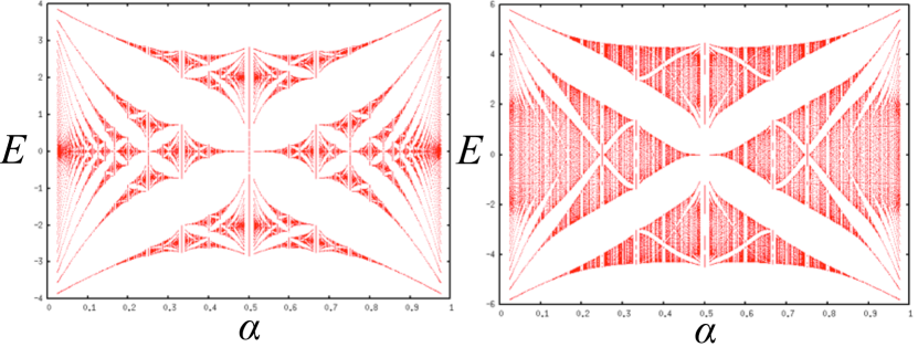
Figure 2: The energy spectrum as function of the magnetic flux $\alpha$ per plaquette, commonly referred as the butterfly spectrum, for the Hofstadter model with $\lambda=t_{y}/t_{x}=1,2$ respectively.

For a moderately deep square optical lattice, the dynamics of (spinless) fermionic atoms in the presence of an artificial magnetic field is described by the tight binding Hamiltonian known as the Hofstadter model [14],

$$H=-\sum_{nm}t_{x}c_{n+1,m}^{\dagger}e^{i\theta_{n+1,m:n,m}}c_{n,m}+t_{y}c_{n,m+1}^{\dagger}e^{i\theta_{n,m+1:n,m}}c_{n,m}+h.c.$$ (1)

where $c_{n,m}$ is the fermion annihilation operator at site $(n,m)$, with $n/m$ is the site index along the $x/y$ direction, $t_{x}$ and $t_{y}$ are the nearest-neighbor hopping along the $x$ and the $y$-direction respectively. The anisotropy in hopping is described by dimensionless parameter $\lambda=t_{y}/t_{x}$. The phase factor $\theta_{n,m:n^{\prime},m^{\prime}}$ is given the line integral of the vector potential ${\bf A}$ along the link from site $(n^{\prime},m^{\prime})$ to $(n,m)$, $(2\pi e/ch)\int{\bf A}\cdot d{\bf l}$. The magnetic flux per plaquete measured in flux quantum is labeled $\alpha$, and represents the strength of magnetic field perpendicular to the 2D plane. The energy spectra for $\lambda=1,2$ are shown in Fig. 2. At commensurate flux, i.e., $\alpha$ is a rational number $\alpha=p/q$ with $p$ and $q$ being integers, the original energy band splits into $q$ sub-bands by the presence of magnetic field, and the spectrum has $q-1$ gaps. For incommensurate flux, namely when $\alpha$ is an irrational number, the fractal spectrum contains a hierarchy of sub-bands with infinite fine structures. As shown in Fig. 2, varying anisotropy changes the size of the gaps without closing any gap.

In the Landau gauge, the vector potential $A_{x}=0$ and $A_{y}=-\alpha x$ and the unit cell is of size $q$ and the magnetic Brillouin zone is $-\pi/q\leq k_{x}\leq\pi/q$ and $-\pi\leq k_{y}\leq\pi$ (the lattice spacing is set to be 1). The eigenstates of the system can be written as $\Psi_{n,m}=e^{ik_{x}n+ik_{y}m}\psi_{n}$ where $\psi_{n}$ satisfies the Harper equation [14],

$$e^{ik_{x}}\psi^{r}_{n+1}+e^{-ik_{x}}\psi^{r}_{n-1}+2\lambda\cos(2\pi n\alpha+k_{y})\psi^{r}_{n}=-E\psi^{r}_{n}.$$ (2)

Here $\psi^{r}_{n+q}=\psi^{r}_{n}$, $r=1,2,...q$, labels linearly independent solutions. The properties of the two-dimensional system can be studied by studying one-dimensional equation (2). For chemical potentials inside each energy gap, the system is in an integer quantum Hall state characterized by its Chern number $c_{r}$ and the transverse conductivity $\sigma_{xy}=c_{r}{e^{2}}/{h}$, where the Chern number of $r$-filled bands is given by,

$$c_{r}=\mathrm{Im}\sum_{r=1}^{l}\int dk_{x}dk_{y}\sum_{n=1}^{q}\partial_{k_{x}}(\psi^{r}_{n})^{*}\partial_{k_{y}}\psi^{r}_{n}.$$ (3)

Here the integration over $k_{x},k_{y}$ is over the magnetic Brillouin zone.

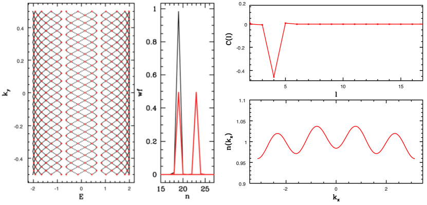
Figure 3: Left: energy spectrum for $\lambda=10$, $\alpha=13/21$ . The red dots indicate dimerized states at the band edges. Middle: the wave function of a state localized at a single site, with energy away from the band edge (black), and the dimerized wave function that localizes at two distinct sites at a distance of four-lattice spacing apart for state at band edge near a gap with Chern number $4$ (red). Figure on the right shows the two point correlation function $C(l)$ that vanishes unless $l=4$ resulting in almost sinusoidal momentum distribution with period $4$.

Chern-Dimer mapping for anisotropic lattices

As illustrated in Fig. (2), the hopping anisotropy changes the size of the gaps, without ever closing the gap. Hence the topological aspects of the underlying states are preserved, as $\lambda$ is continuously tuned. In the limit $\lambda\gg 1$, the problems becomes tractable using degenerate perturbation theory [15]. For $\lambda\rightarrow\infty$, the $q$ bands have dispersion $E_{r}(k_{y})=-2t_{y}\cos(2\pi\alpha r+k_{y})$, $r\in\left\{1,\ldots,q\right\}$. These eigenstates are extended along $y$ but localized to single sites as a function of $x$, with wave function $\psi^{r}_{n}=\delta_{n,r}$. These cosine bands shifted from each other intersect at numerous degeneracy points ${k^{*}_{y}}$. For finite $\lambda$, the hopping term proportional to $t_{x}$ hybridizes the two states at each crossing, resulting an avoided crossing as shown in Fig  (4). Near each degeneracy point the system is well described by a two-level effective Hamiltonian [15],

$${H}(\mathbf{k})=\Delta_{\ell}[\cos(k_{x}\ell){\sigma}_{x}+\sin(k_{x}\ell){\sigma}_{y}]+v_{\ell}(k_{y}-k^{*}_{y}){\sigma}_{z}.$$ (4)

Here ${\sigma}_{x,y,z}$ are the Pauli matrices in the space of localized states $\mathinner{|{r}\rangle}$ and $\mathinner{|{r^{\prime}}\rangle}$, and $\ell=r^{\prime}-r$ is the spatial separation between these two localized states. The expression for $\Delta_{\ell}$ and $v_{\ell}$ are given in Ref. [16]. The eigenstates are equal-weight superpositions of $\mathinner{|{r}\rangle}$ and $\mathinner{|{r^{\prime}}\rangle}$,

$$\psi^{\pm}_{n}=\frac{1}{\sqrt{2}}\left(\delta_{n,r}+e^{i\beta_{\pm}}\delta_{n,r^{\prime}}\right),$$ (5)

where $\beta_{+}=-\ell(k_{x}+\pi)+\pi$ and $\beta_{-}=-\ell(k_{x}+\pi)$ are relative phases for the upper and lower band edges, respectively. We call such dimerized state “Chern-dimers”. Starting from Eq. (5), it is straightforward to show [15] that the corresponding Chern number is related to the phase factor $e^{ik_{x}\ell}$, and simply given by $c_{r}=\ell$. Thus, for sufficiently anisotropic hopping, dimerized states form at the band edges with its spatial extent along $x$ equal to the Chern number of the corresponding gap. Such one-to-one correspondence between the Chern number and the size of the real space dimer (in the Landau gauge) will be referred to as “Chern-dimer mapping”. While calculation of Chern number in this limit is not new, this mapping has not been elucidated and emphasized until our work [16].

The formation of Chern-dimers of size $\ell=c_{r}$ at the edges of the $r$-th gap implies a “hidden spatial correlation”. The correlation function

$$C(l)=\sum_{n,m}\langle c^{\dagger}_{n,m}c_{n+l,m}\rangle$$ (6)

will peak at $l=\ell=c_{r}$. For chemical potential in the $r$-th gap, as $\lambda\rightarrow\infty$, ( Fig.  4) $C(l)$ asymptotes to a delta function $C(l)\rightarrow\delta(l-\ell)$, due to the contribution of Chern-dimers at the lower edge of the $r$-th gap. Note that the net contribution to $C(l)$ from all other dimerized states associated with gaps fully below the Fermi energy is zero, because $\beta_{+}-\beta_{-}=\pi$ for each of these crossings. Remarkably, $C(l)$, or more precisely its Fourier transform $n(k_{x})$, is directly accessible in the time-of-flight (TOF) image, an routine observable in cold atom experiments,

In the time-of-flight experiments, the artificial gauge field is first turned off abruptly. This introduces an impulse of effective electric field that converts the canonical momentum of atoms (when gauge field was on) into the mechanical momentum (these subtleties are discussed in [16]). Then the optical lattice and trap potential are turned off, the density of the atomic cloud $n(\mathbf{x})$ is imaged after a period of free expansion $t_{\rm TOF}$. The image is a direct measurement of the (mechanical) momentum distribution function with ${\bf k}=m{\bf x}/\hbar t_{\rm TOF}$,

$$n(\mathbf{k})=\sum_{\mathbf{r,r^{\prime}}}\langle c^{\dagger}_{\mathbf{r}}c_{\mathbf{r^{\prime}}}\rangle e^{i\mathbf{k}\cdot(\mathbf{r-r^{\prime}})},$$ (7)

where the site label $\mathbf{r}=m\hat{x}+n\hat{y}$, and for simplicity we neglect the overall prefactor and the Wannier function envelope. Thus, from TOF images, the 1D momentum distribution can be constructed by integrating $n({\bf k})$ over $k_{y}$, $n(k_{x})=\int_{-\pi}^{\pi}dk_{y}{n}({\bf k})$, which is nothing but the Fourier transform of $C(l)$. Thus, in the limit of large $\lambda$, $C(l)$ becomes a delta function, and the 1D momentum distribution function becomes

$$n(k_{x})=r\pm\frac{1}{2}\cos(c_{r}k_{x})+...$$ (8)

It assumes a sinusoidal form, with oscillation period given by the Chern number. Note the sign depends on which gap the chemical potential lies in [16], and the off-set $r$ comes from the contribution from the filled bands below the Fermi energy. In summary, we have arrived at the conclusion that Chern numbers can be simply read off from $n(k_{x})$ as measured in TOF, in the large anisotropy limit.

Chern number in time-of-flight images

We now address the question whether it is still possible to extract $c_{r}$ from TOF when away from the large $\lambda$ limit. Note that, while the Chern number does not change inside the same gap as $\lambda$ is tuned, $n(k_{x})$ is not topologically invariant. There is a prior no reason to expect Chern number continues to leave its fingerprints in $n(k_{x})$. Motivated by these considerations, we have carried out detailed numerical studies of momentum distribution in the entire $\alpha-\lambda$ parameter plane, going well beyond the “Chern-dimer regime”. Fig.  (4) highlights our results with various $\lambda$ but fixed $\alpha$ and Chern number. As $\lambda$ is reduced, $n(k_{x})$ gradually deviates from the sinusoidal distribution. Yet, the local maxima (peaks) persist. In the limit of isotropic lattice, $n(k_{x})$ shows pronounced local peaks. For a wide region of parameters, we can summarize our finding into an empirical rule: the number of local peaks in $n(k_{x})$ within the first Brillouin zone is equal to the Chern number. Note that this rule is not always precise, as seen in the Fig. (4) for the case of Chern number $3$ for intermediate values of $\lambda$ where local peaks become a broad shoulder-like structure. Despite this, it is valid in extended regions including both large $\lambda$ and $\lambda=1$. In fact, given the reasoning above, our empirical rule seems to work surprisingly well. But this is an encouraging result for cold atoms experiments. From these distinctive features in $n(k_{x})$, the Chern number can be determined rather easily by counting the peaks, especially for the major gaps with low Chern number.

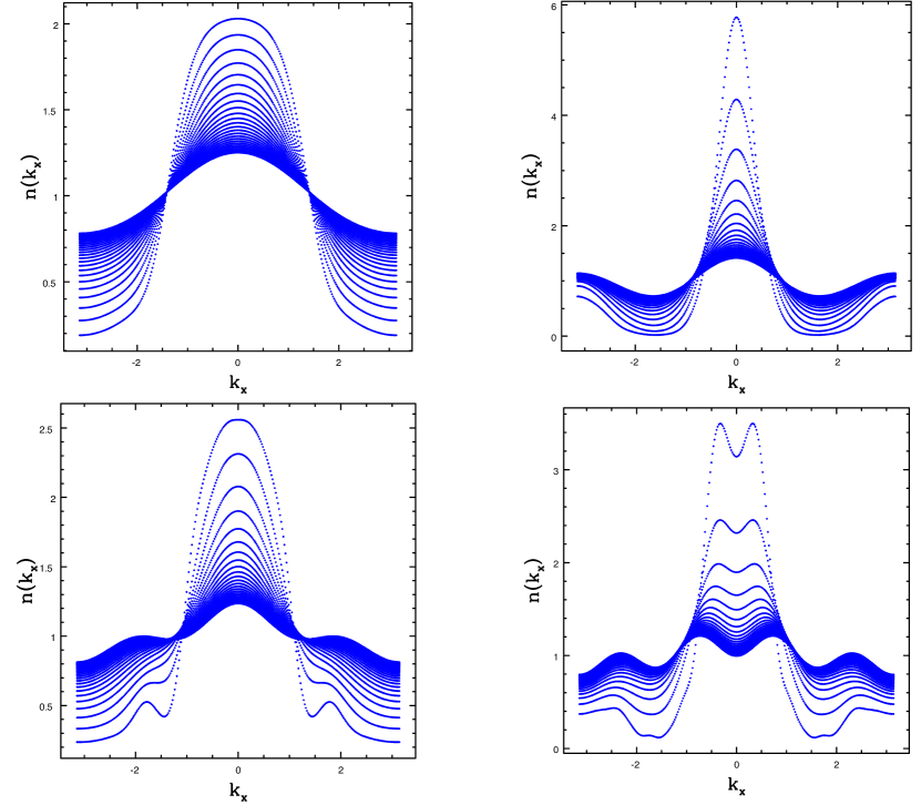
Figure 4: Momentum distribution as anisotropy parameter varies from $1-10$, for $\alpha=.45$ for chern numbers $1$ (top-left), $2$ (top-right), $3$ (bottom-left), and $4$ (bottom-right).

The Chern-dimer mapping provides a simple, intuitive understanding of $n(k_{x})$ in the limit of large $\lambda$. For the isotropic case, there is no dimerization, why are there pronounced peaks in $n(k_{x})$, and why is the peak number precisely equal to the Chern number? To obtain further insight, we considered the low flux limit, $\alpha\rightarrow 0$, where the size of the cyclotron orbit is large compared to the lattice spacing, and the system approaches the continuum limit. The spectrum then can be approximated by discrete Landau levels. For $r$ filled Landau levels, $n(k_{x})$ can be obtained rather easily,

$$n(k_{x})=\sum_{\nu=0}^{r-1}(2^{\nu}\nu!)^{-1}H^{2}_{\nu}({k_{x}})e^{-k^{2}_{x}},$$ (9)

where $H_{\nu}$ is the Hermite polynomial, and $k_{x}$ is measured in the inverse magnetic length $\sqrt{eB/\hbar c}$. $n(k_{x})$ is given by the weighted sum of consecutive positive-definite function, $H^{2}_{\nu}({k_{x}})$. The node structure of $H_{\nu}$ is such that $n(k_{x})$ has exactly $r$ local maxima (peaks) for $r$ filled Landau levels. This nicely explains the numerical results for the Hofstadter model at low (but finite) flux $\alpha=1/q$, where the Chern number $c_{r}=r$ in the $r$-th gap, and $n(k_{x})$ has precisely $r$ peaks (see Fig. 5). Note that this calculation does not directly explain the feature shown in Fig. 4 for $\alpha=0.45$ and $\lambda=1$. As $\alpha$ increases, for $\mu$ residing within the same energy gap, the distinctive features of $n(k_{x})$ are generally retained, so the counting rule is still valid. Compared to the low flux regime, however, the local peaks (except the one at $k_{x}=0$) move to higher momenta.

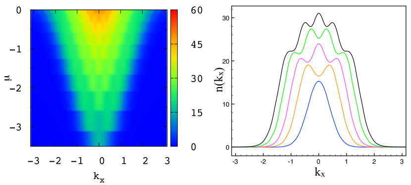
Figure 5: Left: $n(k_{x},\mu)$ in false color for a $50\times 50$ lattice with isotropic hopping and flux $\alpha=0.05$. Right: $n(k_{x})$ for chemical potential $\mu/t$=-3.4, -2.8, -2.4, -1.8, -1.5 respectively (bottom to top). The corresponding Chern number is 1, 2, 3, 4, and 5.

Incommensurate flux: Chern tree

While it is numerically straightforward to investigate the $n(k_{x})$ or $\sigma_{xy}$ for QHE at incommensurate flux $\alpha$, analytical analysis of the Chern number for this case represents a conceptual as well as a technical challenge. In fact, for irrational $\alpha$, the system no longer has translational symmetry, and the notion of magnetic Brillouin zone or Bloch wave function lose their meaning. The incommensurability acts like correlated disorder. The TKNN formula for a periodic system is not directly applicable. In addition, the energy spectrum becomes infinitely fragmented (a Cantor set). One expects then a dense distribution of Chern numbers even within a small window of energy. Then two questions arise. First, will these Chern numbers largely random or are there deterministic patterns governing their sequence as $\mu$ is continuously varied? Second, what is the experimental outcome of $n(k_{x})$ or $\sigma_{xy}$ when measured with a finite energy resolution?

We address some of these questions here for the isotropic lattice ($\lambda=1$) using the golden-mean flux, $\alpha=(\sqrt{5}-1)/2$, as an example. We will employ a well known trick, and approach the irrational limit by a series of rational approximation $\alpha_{n}=F_{n}/F_{n+1}$, where $F_{n}$ is the $n$-th Fibonacci numbers. Explicitly, the series $3/5,5/8,8/13,13/21,21/34,34/55,55/89...$ approaches the golden-mean with increasing accuracy. At each stage of the rational approximation, the energy spectrum and the corresponding sequence of Chern numbers can be determined. Higher Chern numbers are typically associated to smaller gaps in the asymptotically fractal spectrum. At first sight, the Chern number associated with the $r$-th gap seems an irregular function of $r$ as shown in Fig. (6) for $\alpha=34/55$. This is in sharp contrast with the case of $\alpha=1/q$, where $c_{r}=r$ for the $r$-th gap.

Now we show analytically that there actually exists a deterministic pattern underlying the sequence of Chern numbers. This pattern follows from the solutions of the Diophantine equation (DE)[12], $r=c_{r}p+s_{r}q$, where $r$ is the gap index, $c_{r}$ is the Chern number, at each level of the rational approximation, $p=F_{n},q=F_{n+1}$. We first classify all the Chern numbers into two classes, the Fibonacci Chern numbers and the non-Fibonacci Chern numbers. All the solutions to the DE, which determine the Chern number, can be exhausted by following two simple rules, labeled as I, II and explicitly stated below.

(I) Fibonacci Chern numbers occur at gaps labeled by a Fibonacci index $r=F_{m}$: for $\alpha=F_{n-1}/F_{n}$, $c_{r=F_{m}}=-(-1)^{n-m}F_{n-m}$ . Here $r=1$ corresponds to the first gap near the band edge with Chern number $F_{n-2}=(-1)^{n_{f}}(q-p)$, while the last Fibonacci gap near the band center has a Chern number $(-1)^{n_{f}}$ where $n_{f}$ counts the number of Fibonacci numbers less than $|{q}/{2}|$. The Fibonacci Chern numbers increases monotonically in magnitude as one moves from the center towards the edge of the band (see Fig. 6).

(II) The rest are the non-Fibonacci Chern numbers. The Chern number for the $r$-th gap and its neighboring gaps ($r\pm 1$) obey the recursion relation,

$$c_{r} = {(c_{r+1}+c_{r-1})}/{2},$$

$$c_{r+1} = c_{r}+(-1)^{n_{f}}(q-p),$$

$$c_{r-1} = c_{r}-(-1)^{n_{f}}(q-p),$$

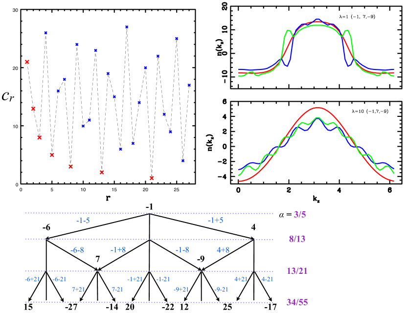
Figure 6: The Chern tree at golden-mean flux showing four consecutive rational approximations: $\alpha=3/5,8/13,13/21,34/55$ starting with Chern number $-1$. The horizontal axis is not to scale and only shows the correct order of Chern numbers. Top-left figure shows Fibonacci (red) and non-Fibonacci (blue) Chern numbers vs the gap index $r$ for $\alpha=34/55$. Top-right shows momentum distribution for three different topological states characterized by Chern numbers $1$ (red), $7$ (blue) and $-9$ (green). Figure illustrates self-averaging aspect of the momentum distribution: states $7$ and $-9$ that reside in close proximity to the state with Chern number unity have ripples that tend to cancel each other.

Following these rules, we can construct an exhaustive list of all Chern numbers at each level of rational approximation. We have numerically checked that the Chern numbers computed from the TKNN formula are consistent with the predictions from the DE above. This procedure yields a hierarchy of Chern numbers, which can be neatly organized into a tree structure, thanks to the recursion relation above. A subset of this tree hierarchy is shown in Fig. 6. Most notably, we find the average of the left and right neighboring Chern number is exactly the Chern number in the middle.

This property helps to understand the measurement outcomes of real experiments, which inevitably involves average of states with energy very close to each other. In the context of cold atoms, due to the overall trap potential, the local chemical potential slowly varies in space. These local contributions sum up in TOF images according to the local density approximation. The self-averaging property to some degree ensures that such average yields definite result, and the infinitely fine details in the energy spectrum are largely irrelevant. This aspect is illustrated in Fig. 6 for the Chern tree shown in Fig. 6. The momentum distribution $n(k_{x})$ in the average sense for $\alpha=3/5,8/13,13/21,34/55$ will be essentially the same.

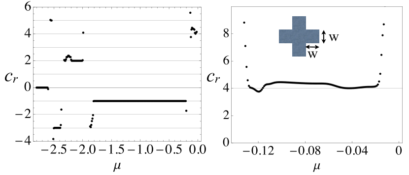
Figure 7: Left: the quantized conductance $c_{r}=\sigma_{xy}/(e^{2}/h)$ versus the chemical potential $\mu$ for $\lambda=1$ and $\alpha=(\sqrt{5}-1)/2$. Right: the blow up for $\mu$ close to zero showing an extended plateau at $c_{r}=4$. $c_{r}$ is computed for a four-terminal quantum Hall bar of width $W=20a$ (inset). The device is connected to four semi-infinite leads of the same material with inelastic scattering rate $0.005t$.

Similar consideration applies to $\sigma_{xy}$. One may see a robust plateau, which may not be perfectly quantized, in a region of chemical potential due to the self-averaging. We have numerically computed $\sigma_{xy}$ using the Landauer-Buttiker formalism [18] for a mesoscopic quantum Hall bar (inset of Fig. 7) at golden-mean flux and connected to four semi-infinite leads. The transmission coefficients $T_{ij}$ are obtained by solving for the Green’s function of the sample and the level width functions of each leads. The transverse conductivity at golden-mean flux is shown in Fig. 7. One clearly sees a conductance plateau with $c_{r}=4$, in addition to $c_{r}=1,2,3$.

Quantum spin Hall effect for ultracold atoms

In solid state, the QSH effect is closely related to spin-orbit coupling. In a recent study [17], it was shown that the effect of spin-orbit coupling can be achieved for cold atoms by creating $SU(2)$ artificial gauge fields.

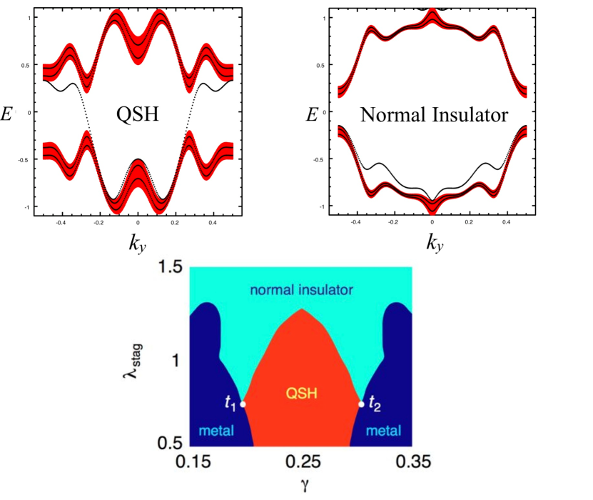
Figure 8: Shows the bulk (red) and surface spectrum (black) , near half-filling, for $\alpha=1/6$, $\gamma=.25$, $\lambda=1$ , and $\lambda_{stag}=.5$ ( left) and $\lambda_{stag}=1.5$ ( right). The presence of gapless edge modes for $\lambda_{stag}=.5$ and their absence for $\lambda_{stag}=1.5$ shows that these two respectively correspond to topologically non-trivial and trivial phases. The bottom caption shows the corresponding Phase diagram in $\gamma-\lambda_{stag}$ plane .

The theoretical model that captures the essential properties of this system is given by a Hamiltonian describing fermions hopping on a square lattice in the presence of a SU(2) gauge field

$$\mathcal{H}=-t\sum_{mn}\bf{c}_{m+1,n}^{\dagger}e^{i\theta_{x}}\bf{c}_{m,n}+\bf{c}_{m,n+1}^{\dagger}e^{i\theta_{y}}\bf{c}_{m,n}+h.c.+\lambda_{stag}(-1)^{m}\,\bf{c}^{\dagger}_{m,n}\bf{c}_{m,n}$$ (10)

where $\bf{c}_{m,n}$ is the 2-component field operator defined on a lattice site $(m,n)$, and $\lambda_{stag}$ is the onsite staggered potential along the $x$-axis. The phase factors $\theta_{m,n}$ corresponding to $SU(2)$ gauge fields are chosen to be,

$$\theta_{x} = 2\pi\gamma{\bf\sigma_{x}},$$

$$\theta_{y} = 2\pi x\alpha{\bf\sigma_{z}},$$ (11)

where ${\bf\sigma_{x,z}}$ are Pauli matrices. The control parameter $\gamma$ is a crossover parameter between QH and QSH states as $\gamma=0$ describes uncoupled double QH systems while $\gamma=\pi/2$ corresponds to the two maximally coupled QH states. It should be noted that the Hamiltonian (10) is invariant under time-reversal. The two components of the field operators correspond in general to a pseudo-spin 1/2, but could also refer to the spin components of atoms, such as ⁶Li, in a $F=1/2$ ground state hyperfine manifold. For $\gamma=0$ case, spin is a good quantum number and the system decouples into two subsystems which are respectively subjected to the magnetic fluxes $\alpha$ and $-\alpha$.

For isotropic lattices, this Multiband system has been found to exhibit[17] a series of quantum phase transitions between QSH, normal insulator and metallic phases in two-dimensional parameter space for various values of chemical potential. Figure  (9) shows the landscape of the phases near half-filling for $\alpha=1/6$. The transitions from topologically nontrivial quantum spin Hall (QSH) to topologically trivial normal band insulator is signaled by the disappearance of gapless Kramer-pair of chiral edge modes.

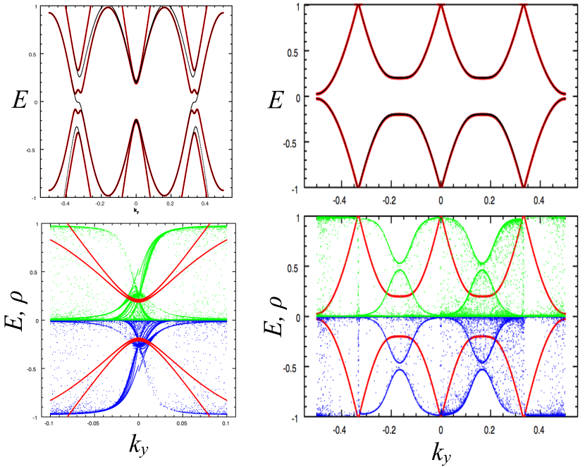
Figure 9: Figure illustrates quantum phase transition from topologically non-trivial state ( indicated by gapless edge modes ) to normal insulating state. for $\gamma=.25$, $\lambda=5$ , and $\lambda_{stag}=5$ ( top-left) and $\lambda_{stag}=10$ (right). In the bottom caption, Green and blue show the local density of the two-component state at all sites. For normalized spinor wave function, a density of $.25$ shows the existence of a dimerized state for each component of the spinor.

Motivated by the fact that anisotropic lattices, reveal a novel type of encoding of nontrivial topological states in the form of “Chern-Dimers”, for $U(1)$ gauge systems, we present our preliminary results of QSH states for anisotropic lattices. As shown in the Fig.  9, anisotropic lattices subjected to $SU(2)$ gauge fields exhibit quantum phase transitions from QSH to normal insulating state by tuning the staggered potential. In contrast to the QH system, the avoided crossings in QSH system need not be isolated as seen near $k_{y}=1/3$. However, there are states, such as those near $k_{y}=0$ where one sees an isolated avoided crossing.

Our preliminary investigation as summarized in figure  (9) shows that for anisotropic lattices, in QSH phase, both components of the spinor wave function are dimerized near an isolated avoided crossings. It is the existence of this double or spinor-dimer that distinguishes QSH state from a normal insulator. In other words, each component of the wave function of topologically non-trivial insulating phase localizes at two distinct sites, which is in contrast to the topologically trivial phase, where the-components of the wave functions localize at a single site. For normalized states, the existence of a double-dimer can be spotted by density approaching $.25$ as illustrated in the Fig. 9. The distinction between the QSH and normal insulator, characterized by spinor-dimer and its absence suggests that such topological phase transitions may be identified by time of flight images.

Open questions and outlook

Identifying topological states in time of flight images would be a dream measurement for cold atom experimentalists. Therefore, our result that the momentum distribution carries fingerprints of nontrivial topology is important.

Our studies raise several open questions regarding topological states and its manifestations. Firstly, our detailed investigation suggests that the features of topological invariant (Chern number) in momentum distribution are quite robust. Is there a rigorous theoretical framework that can establish this connection even for parameters beyond Chern-dimer regime? Secondly, the sign of the Chern number can not be directly determined from the momentum distribution. It remains an open question whether some other observable can detect its sign.

Another natural question is: how generic is the existence of dimerized states in topological states of matter? Somewhat analogous to edge states, the size of the dimerized states in our example is a robust (topologically protected) quantity. Furthermore, are edge states and dimerized states related to each other? Naively, one expects a dimer of size $N$ in bulk will result in $N$-possible types of defects at open boundaries. These “defects” quite possibly will manifest as edge states inside the gap. It is conceivable that the topological aspect of the dimers of size $N$ is intimately related to $N$-edge states in QH systems. Further work is required to test these speculations, even in special cases.

To investigate the generality of the dimer framework in topological states, we have studied QSH states for anisotropic lattices. Our preliminary studies suggest that the topological phase transition from QSH to normal insulating state is accompanied by the absence of dimerized states and hence may be traceable in time of flight images. Detailed characterization of $Z_{2}$ invariance within the framework of spatially extended objects, however remains appealing but open problem.

The subject of topological states of matter is an active frontier in physics. Lessons learned from their realizations in ultracold atoms will help to advance the fundamental understanding, and inspire new material design or technological applications. Ultracold topological superfluids, Mott insulators with nontrivial topology, and non-equilibrium topological states are most likely to bear fruit in reasonably near future.

We thank Noah Bray-Ali, Nathan Goldman, Ian Spielman, and Carl Williams for collaboration and their contributions during the course of this research. We acknowledge the funding support from ONR and NIST.

Index

Chern number….3,6,7
Chern-Dimer mapping….6
Chern tree…. 11, 12, 13
Fibonacci numbers….. 12
Harper equation…..5
Hofstadter model….4
Incommensurate flux….11
Landau-level……9

References

- [1] Y.-J. Lin, R. L. Compton, K. J. Garcia, J. V. Porto, and I. B. Spielman, Nature 462, 628 (2009)
- [2] Y.-J. Lin, K. Jimenez-Garcia, and I. B. Spielman, Nature 471, 83-86 (2011)
- [3] M. Z. Hasan and C. L. Kane, Rev. Mod. Phys. 82, 3045 (2010).
- [4] A. P. Schnyder, S. Ryu, A. Furusaki, and A. W. W. Ludwig, Phys. Rev. B 78, 195125 (2008).
- [5] A. Kitaev, American Institute of Physics Conference Series, vol. 1134, 22 (2009).
- [6] X.-L. Qi, T. L. Hughes, and S.-C. Zhang, Phys. Rev. B 78, 195424 (2008).
- [7] X.-L. Qi and S.-C. Zhang, Physics Today 63, 33 (2010).
- [8] X. Qi and S. Zhang, ArXiv:1008.2026 (2010).
- [9] N. Cooper, Advances in Physics 57, 539 (2008).
- [10] J. Dalibard, G. Juzeliuna, and P.Öhberg, arxiv:1008.5378 (2010).
- [11] K. v. Klitzing, G. Dorda, and M. Pepper, Phys. Rev. Lett. 45, 494 (1980).
- [12] D. J. Thouless, M. Kohmoto, M. P. Nightingale, and M. den Nijs, Phys. Rev. Lett. 49, 405 (1982).
- [13] C. L. Kane and E. J. Mele, Phys. Rev. Let. 95, 146802 (2005).
- [14] D. R. Hofstadter, Phys. Rev. B 14, 2239 (1976).
- [15] E. Fradkin, Field Theories of Condensed Matter Systems, Addison Wesley, page 287-292.
- [16] E. Zhao, N. Bray-Ali, C. Williams, I. Spielman, and I. Satija, Phys Rev A, 84, 063629 (2011).
- [17] N. Goldman, I. Satija, P. Nikolic, A. Bermudez, M. A. Martin-Delgado, M. Lewenstein, and I. B. Spielman, Phys. Rev. Lett. 105, 255302 (2010)
- [18] M. Buttiker, Phys. Rev. B 38, 9375 (1988).
Index