Adapting Predictive Feedback Chaos Control for Optimal Convergence Speed

Abstract

Stabilizing unstable periodic orbits in a chaotic invariant set not only reveals information about its structure but also leads to various interesting applications. For the successful application of a chaos control scheme, convergence speed is of crucial importance. Here we present a predictive feedback chaos control method that adapts a control parameter online to yield optimal asymptotic convergence speed. We study the adaptive control map both analytically and numerically and prove that it converges at least linearly to a value determined by the spectral radius of the control map at the periodic orbit to be stabilized. The method is easy to implement algorithmically and may find applications for adaptive online control of biological and engineering systems.

I Introduction

Some chaotic attractors contain infinitely many unstable periodic orbits. These can be seen as a “skeleton” for the chaotic attractor, therefore revealing important information about the dynamics of the system itself. By suitable perturbations the stability of these unstable periodic points can be changed; a control perturbation renders them stable. Such “chaos control” has applications in many fields Scholl2007 , including biological Rabinovich1998 and artificial neural networks Steingrube2010 ; Scholl2010 .

In the last twenty years, different methods for stabilizing unstable periodic orbits have been suggested. The seminal work by Ott, Grebogi, and Yorke (OGY) Ott1990 and its implementations employ arbitrary small perturbations of a parameter of the system to stabilize a known unstable periodic orbit of a discrete time dynamical system. A successful application of the OGY method, however, requires prior knowledge about or online analysis of the dynamics to determine fixed points and their stability properties.

A different approach is given by predictive feedback control (PFC) DeSousaVieira1996 ; Polyak2005 which overcomes this disadvantage. In this approach the future state of the dynamics calculated from the current state is fed back into the system to stabilize a periodic orbit. This feedback control is noninvasive, i.e., the control strength vanishes upon convergence, and is extremely easy to implement. It is a special case of a recent effort to stabilize all periodic points of a discrete time dynamical system Schmelcher1997 ; Schmelcher1998 which is also closely related to nonlinear successive over-relaxation methods Yang2010 ; Brewster1984 . It has been extensively studied Diakonos1998 ; Pingel2000 ; Pingel2004 ; Crofts2006 ; Crofts2009 and extended Doyon2002 ; Davidchack1999 with respect to its original purpose as a tool for examining the structure of chaotic attractors.

In any real world application, speed of convergence is of crucial importance. For example, if a robot is controlled by stabilizing periodic orbits in a chaotic attractor Steingrube2010 , the time it needs to react to a changing environment is bounded by the time the system needs to converge to a periodic point of a given period. Hence, in praxis, one desires to tune the control parameter such that the spectral radius of the unknown periodic point which the system converges to is minimized. To the best of our knowledge, previous works on chaos control have not considered convergence speed while maintaining its simplicity in terms of implementation. Adaptation of the control parameter has an impact on convergence speed. However, existing adaptation mechanisms Steingrube2010 ; Lehnert2011 have two major shortcomings; they do not optimize for speed and, for adaptation of heuristic nature, may adapt the parameter to regimes where stabilization fails.

Here we introduce an adaptation method that overcomes these shortcomings. It adaptively tunes the control parameter online to achieve optimal asymptotic convergence speed. This work is organized as follows. In the second section we review the PFC method and introduce the notation that will be used throughout the paper. In the third section, we present the adaptation method and prove its convergence properties. As an example, the well-known logistic map is studied both analytically and numerically in Sections 4 and 5 before giving some concluding remarks.

II Preliminaries

A differentiable map $f:\mathbb{R}^{n}\to\mathbb{R}^{n}$ gives rise to a dynamical system through the evolution equation

$$x_{k+1}=f(x_{k})$$ (1)

with $x_{k}\in\mathbb{R}^{n}$ for all $k\in\mathbb{Z}$. The sequence $(x_{k}),k\in\mathbb{N}$ is called an orbit of the dynamical system with initial condition $x_{0}$ and if $f^{\circ p}(x_{k})=x_{k+p}$ for all $k\geq 0$ we say that the orbit is periodic with period $p$. Here,

$$f^{\circ p}=\underbrace{f\circ f\circ\cdots\circ f}_{p\text{ times}}$$

denotes the $p$-fold composition of $f$. Let $\operatorname{Fix}(f):=\left\{x\in\mathbb{R}^{n}\ \left|\ f(x)=x\right.\right\}$ be the set of fixed points, i.e., periodic points of period one. Note that any periodic orbit is a fixed point of the $p$-th iterate of the map $f$ so we will use the expressions fixed point and periodic orbit interchangeably.

Let $A\subset\mathbb{R}^{n}$ be a forward invariant subset of $\mathbb{R}^{n}$ with respect to $f$, i.e., $f(A)\subset A$. If periodic points are dense in $A$ and $f$ maps transitively, then we call $A$ a chaotic set. Julia sets Milnor2006 , as described below, are examples of such chaotic sets. Let $\mathrm{d}f|_{x}$ denote the derivative of $f$ at $x\in\mathbb{R}^{n}$ and $\operatorname{id}:\mathbb{R}^{n}\to\mathbb{R}^{n}$ the identity map.

The results of Schmelcher1998 are now summarized as follows:

Proposition II.1.

Suppose ${x^{*}}\in\operatorname{Fix}(f)$ and the derivative $\mathrm{d}f|_{{x^{*}}}$ and $\mathrm{d}f|_{{x^{*}}}-\operatorname{id}$ are real, nonsingular and diagonalizable. Then there exist parameters $\mu>0$ and an orthogonal matrix $C_{k}\in O(n)$ such that ${x^{*}}$ is an attractive fixed point of the map $g_{\mu}$ obtained from $f$ through the transformation

$$S(\mu,C_{k}):f\mapsto\operatorname{id}+\mu C_{k}(f-\operatorname{id})=:g_{\mu}.$$

In particular, $S(\mu,C_{k})$ preserves the set of fixed points, that is $\operatorname{Fix}(f)=\operatorname{Fix}(g_{\mu}).$

In fact, it can be shown that the number of matrices $C_{k}$ needed to stabilize all fixed points of a given map $f$ is quite limited. They depend on the local stability properties of fixed points and there are types of fixed points that can be stabilized for $C_{k}\in\left\{\pm\operatorname{id}\right\}$. For a given ${x^{*}}\in\operatorname{Fix}(f)$ with $\chi_{j}\in\mathbb{C}$, $j\in\left\{1,\ldots,n\right\}$, being the eigenvalues of $\mathrm{d}g_{\mu}|_{{x^{*}}}$ we want to denote by

$$\rho_{{x^{*}}}(\mu):=\max_{j\in\left\{1,\ldots,n\right\}}\left\{\left|\chi_{j}\right|\right\}$$

the spectral radius, i.e., the maximum of the absolute values of the eigenvalues of the derivative of $g_{\mu}$ at ${x^{*}}$. We have

$$\mathrm{d}g_{\mu}|_{x}=\operatorname{id}+\mu C_{k}(\mathrm{d}f|_{x}-\operatorname{id}).$$ (2)

for all $x\in\mathbb{R}^{n}$. In other words, the proposition above ensures the existence of $\mu$ and $C_{k}({x^{*}})$ for a given ${x^{*}}\in\operatorname{Fix}(f)$ such that the transformation $S(\mu,C_{k})$ gives $\rho_{{x^{*}}}(\mu)<1$, cf. Figure 1. Therefore, with these parameters, the fixed point ${x^{*}}$ of $f$ is an attracting fixed point for $g_{\mu}$.

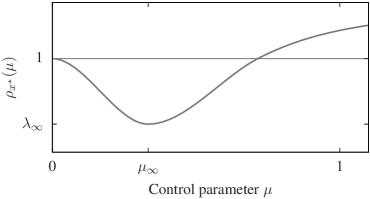
Figure 1: Sketch of the dependence of the spectral radius $\rho_{{x^{*}}}(\mu)$ on $\mu$ for some fixed point ${x^{*}}$ according to Proposition II.1.

The results above are directly related to predictive feedback chaos control methods. A transformation $T_{\eta}:f\mapsto g$ is called a chaos control transformation if $g$ can be written as $g=f+\eta c$ with control perturbation $c:\mathbb{R}^{n}\to\mathbb{R}^{n}$ and $\eta\in\mathbb{R}$. Note that in case $C_{k}\in\left\{\pm\operatorname{id}\right\}$ the transformations $S(C_{k},\mu)$ are chaos control transformations since

$$g_{\mu}=f+(1\mp\mu)(\operatorname{id}-f)$$

with $\eta=1-\mu$. Therefore, we will refer to these transformations $S(\mu,C_{k})$ as PFC transformations. Without loss of generality we restrict ourselves to the case $C_{k}=\operatorname{id}$.

The results of Proposition II.1, however, give little information about the speed of convergence, except for the fact that when decreasing $\mu$ towards zero convergence takes longer and longer as the spectral radius approaches one. In the vicinity of a stabilized fixed point, convergence is at least linear and the rate of convergence is bounded from above by the quantity $\rho_{{x^{*}}}(\mu)$. In order to obtain an adaptation method that increases the speed of convergence we therefore have to minimize $\rho_{{x^{*}}}(\mu)$ using the control parameter $\mu$. For a random initial condition, we do not know to what fixed point ${x^{*}}$ (if any) the trajectory will converge to. We only have a converging sequence $x_{k}\to{x^{*}}$. In other words, we are looking for a way to obtain a sequence $\mu_{k}\to\mu_{\infty}$ where

$$\mu_{\infty}=\sup\left\{\mu>0\ \left|\ \forall\tilde{\mu}>0:\rho_{{x^{*}}}(\mu)\leq\rho_{{x^{*}}}(\tilde{\mu})\begin{array}[]{l}\text{and assumptions of}\\ \text{Prop.\leavevmode\nobreak\ \ref{prop:SD} are satisfied}\end{array}\right.\right\}$$ (3)

the optimal $\mu$ to minimize $\rho_{{x^{*}}}(\mu)$. Define $\lambda_{\infty}:=\rho_{{x^{*}}}(\mu_{\infty})$.

In applications, the control parameter $\mu$ plays a double role; on the one hand, it can be used to turn chaos control on and off, $\mu=1$, on the other hand it is the crucial parameter to stabilize the periodic orbits and to determine the speed of convergence.

Define the class of functions

$$\mathcal{F}(\mu_{0},p):=\left\{f\ \left|\ \operatorname{card}\left(\left\{x\in\operatorname{Fix}(f^{\circ p})\ \left|\ \rho_{x}(\mu_{0})<1\text{ for }C_{k}=\operatorname{id}\right.\right\}\right)>0\right.\right\},$$

with parameters $p\in\mathbb{N}$, and $\mu_{0}>0$ and where $\operatorname{card}$ denotes the cardinality of a set. The sets $\mathcal{F}(\mu_{0},p)$ are the functions $f$ with a chaotic set that have at least one periodic orbit of period $p$ which can be stabilized for the given parameters.

III An Adaptation Method to Accelerate Chaos Control

In this section, suppose $f\in\mathcal{F}(\mu_{0},p)$ for some $\mu_{0}>0$ and without loss of generality, $p=1$, since we can replace $f$ with the $p$-th iterate. Suppose $g_{\mu}$ is the transformed map after applying $S(\mu,\operatorname{id})$. Furthermore we assume that for all times $k<0$ the system evolves according to Equation (1), i.e., with $\eta=1-\mu=0$, along a trajectory of points in the chaotic set $A$. At time $k=0$ the control parameter $\mu$ is set to $\mu_{0}$. Therefore, because of the assumptions on $f$, there is at least one periodic orbit of period $p$ on the chaotic attractor which is now an attracting periodic orbit. Let $\operatorname{sFix}(f)$ denote the set of these stabilized fixed points.

III.1 Close to a fixed point

Recall two facts: any differentiable map $h\in\mathcal{C}^{1}(U)$ on an open set $U\subset\mathbb{R}^{n}$ is Lipschitz-continuous on any compact $K\subset U$, that is

$$\left\|h(x)-h(y)\right\|\leq\|\mathrm{d}h\|_{K}\cdot\left\|x-y\right\|,$$

for all $x,y\in K$ where $\|\,\cdot\,\|_{K}$ is the supremum of the operator norms induced by a norm $\|\,\cdot\,\|$ on $K$ and $\mathrm{d}h$ is the total derivative. Furthermore, for any contraction $h$ on a Banach space $(X,\|\,\cdot\,\|)$, i.e., a map that satisfies

$$\left\|h(x)-h(y)\right\|\leq L\left\|x-y\right\|$$

with a Lipschitz constant $L<1$, the Banach Fixed Point Theorem gives the existence of a unique fixed point ${x^{*}}$ together with the error estimates $\left\|{x^{*}}-x_{k}\right\|\leq\frac{L^{k}}{1-L}\left\|x_{0}-x_{1}\right\|$ and $\left\|x_{k+1}-x_{k}\right\|\leq L\left\|x_{k}-x_{k-1}\right\|$. Here, $x_{k}=h^{\circ k}(x_{0})$ for an initial condition $x_{0}\in X$.

Let ${x^{*}}\in\operatorname{sFix}(f)$ be fixed. According to Proposition II.1 there exists a $\lambda_{0}<1$ for $\mu=\mu_{0}$ sufficiently small such that $\rho_{{x^{*}}}(\mu_{0})<\lambda_{0}$. Therefore, there exists a vector norm $\|\ \cdot\ \|$ such that we have $\|\mathrm{d}g_{\mu}|_{{x^{*}}}\|_{\textrm{op}}\leq\lambda_{0}$ for the induced operator norm cf. Figure 2(a). We will omit the index indicating the operator norm when it is clear from the context. Henceforth all norms denote this vector norm and the induced operator norm respectively.

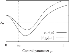
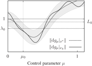
Figure 2: (a) An appropriately chosen norm approximates the spectral radius from above with $\rho_{{x^{*}}}(\mu_{0})\leq\|\mathrm{d}g_{\mu_{0}}|_{{x^{*}}}\|\leq\lambda_{0}$. (b) According to Condition (4), $\|\mathrm{d}g_{\mu}|_{x_{k}}\|$ lies in a $K\left\|{x^{*}}-x_{k}\right\|$-tube around $\|\mathrm{d}g_{\mu}|_{{x^{*}}}\|$. While iterating, this tube becomes smaller and smaller. As another consequence of (4), we have $\|\mathrm{d}g_{\mu}|_{x}\|_{\overline{B(\varepsilon,{x^{*}})}}$ in a $K\varepsilon$-tube around $\|\mathrm{d}g_{\mu}|_{{x^{*}}}\|$. Therefore, for $\varepsilon$ small enough, there is $L_{0}<1$ such that $\|\mathrm{d}g_{\mu_{0}}|_{x}\|_{\overline{B(\varepsilon,{x^{*}})}}\leq L_{0}$.

Let $B(\varepsilon,x)$ denote a ball of radius $\varepsilon$ centered at $x$ and by $\overline{B(\varepsilon,x)}$ its closure. Assume that for $\tilde{\varepsilon}$ small enough there is a constant $K\geq 0$ such that

$$\left|\|\mathrm{d}g_{\mu}|_{x^{*}}\|-\|\mathrm{d}g_{\mu}|_{{x}}\|\right|\leq K\left\|{x^{*}}-{x}\right\|$$ (4)

for all $x$ with $\left\|{x^{*}}-x\right\|<\tilde{\varepsilon}$ independent of $\mu$. This condition is depicted in Figure 2(b). Now we can choose $\varepsilon\leq\tilde{\varepsilon}$ such that $\|\mathrm{d}g_{\mu_{0}}|_{x}\|_{\overline{B(\varepsilon,{x^{*}})}}<1$. Put differently, for sufficiently small $\delta_{0}>0$ there exists an $\varepsilon\in(0,\tilde{\varepsilon})$ such that $\|\mathrm{d}g_{\mu_{0}}|_{x}\|_{\overline{B(\varepsilon,{x^{*}})}}\leq\lambda_{0}+\delta_{0}=:L_{0}<1$. The choice of $\varepsilon$ (corresponding to the size of the ball around ${x^{*}}$) depends on $\lambda_{0}$, $\mu_{0}$, and $\delta_{0}$.

Remark III.1.

Condition (4) is satisfied in case $f$ has a bounded second derivative on $\operatorname{sFix}(f)$ due to the functional dependence of the derivative of $g_{\mu}$ on $\mu$ as given by (2).

Algorithm III.2.

For given $f\in\mathcal{F}(\mu_{0},p),\mu_{0},\lambda_{0},$ and $K$ let $x_{0}\in B(\varepsilon,{x^{*}})$. The convergence acceleration algorithm consists of the following steps:

Step 1

(Iterate): Calculate $x_{1}=g_{\mu_{0}}(x_{0})$.

Step 2

(Optimize $\mu$): Minimize the “cost function” $\|\mathrm{d}g_{\mu}|_{x_{1}}\|$ with respect to $\mu\in(0,1)$ under the conditions

$$l(\mu):=\|\mathrm{d}g_{\mu}|_{x_{1}}\|+\left(\frac{2KL_{0}}{1-L_{0}}\right)\left\|x_{0}-x_{1}\right\|<L_{0}$$ (5a)

$$\mu\text{ maximal}$$ (5b)

where $L_{0}=\lambda_{0}+\delta_{0}$ as above, cf. Figure 3.

Step 3

(Set quantities): If the minimization under constraints of Step 2 returned a result $\mu_{\mathrm{opt}}$ then set $\mu_{1}:=\mu_{\mathrm{opt}},\lambda_{1}:=\|\mathrm{d}g_{\mu}|_{x_{1}}\|+\left(\frac{KL_{0}}{1-L_{0}}\right)\left\|x_{0}-x_{1}\right\|$, $\delta_{1}:=\left(\frac{KL_{0}}{1-L_{0}}\right)\left\|x_{0}-x_{1}\right\|$ and $L_{1}:=\lambda_{1}+\delta_{1}$. Otherwise set $\mu_{1}:=\mu_{0},\lambda_{1}:=\lambda_{0},\delta_{1}:=\delta_{0}$ and $L_{1}:=L_{0}$.

Repeat the steps with all indices increased by one.

For this method we obtain the following results.

Lemma III.3.

With the assumptions of Algorithm III.2 above we have that for any initial condition $x_{0}\in B(\varepsilon,{x^{*}})$ Algorithm III.2 yields a trajectory $x_{k}\to{x^{*}}$.

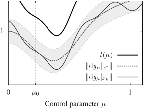
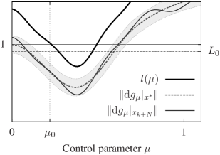
Figure 3: (a) Inequality (5a) does not always have to be satisfied. (b) Since $x_{k}\to{x^{*}}$ we have that after a finite time $N$ the function $l(\mu)$ is below $L_{0}$ for some $\mu$.

Proof.

If the optimization process does not give a result, convergence is ensured by Proposition II.1 and the Banach Fixed Point Theorem. Without loss of generality, suppose that optimization yields a result for $k=1$. Then because of (4) and (5a) we have

$$\|\mathrm{d}g_{\mu_{1}}|_{{x^{*}}}\|_{\overline{B(\left\|x_{1}-{x^{*}}\right\|,{x^{*}})}} \leq\|\mathrm{d}g_{\mu_{1}}|_{{x^{*}}}\|+K\left\|x_{1}-{x^{*}}\right\|$$

$$\leq\|\mathrm{d}g_{\mu_{1}}|_{x_{1}}\|+2K\left\|x_{1}-{x^{*}}\right\|$$

$$\leq\|\mathrm{d}g_{\mu_{1}}|_{x_{1}}\|+\left(\frac{2KL_{0}}{1-L_{0}}\right)\left\|x_{1}-x_{0}\right\|$$

$$=L_{1}\leq L_{0}<1.$$

Therefore, $x_{1}$ is contained in a ball around the fixed point ${x^{*}}$ on which the map $g_{\mu_{1}}$ is a contraction with contraction coefficient $L_{1}$. The same calculation is valid for subsequent optimization steps for $k>1$.   ∎

The lemma above ensures that the adaptation does not compromise convergence against the stabilized fixed point. But will optimization actually take place? For a map with $K=0$, adaptation is not necessary since $\|\mathrm{d}g_{\mu}|_{{x^{*}}}\|=\|\mathrm{d}g_{\mu}|_{x_{k}}\|$ and therefore we can set $\mu$ straight to the optimal value.

Lemma III.4.

With the assumptions of Algorithm III.2 Inequality (5a) is satisfied every finitely many steps.

Proof.

By definition we have $\|\mathrm{d}g_{\mu_{0}}|_{{x^{*}}}\|\leq L_{0}=\lambda_{0}+\delta_{0}$ with $\delta_{0}>0$. Hence we have $\|\mathrm{d}g_{\mu_{0}}|_{{x^{*}}}\|<L_{0}$. Let $\zeta>0$ be such that $\zeta<L_{0}-\|\mathrm{d}g_{\mu_{0}}|_{{x^{*}}}\|$. Since $\left\|x_{k}-x_{k+1}\right\|$ is a Cauchy sequence and $\|\mathrm{d}g_{\mu_{0}}|_{x_{k}}\|\to\|\mathrm{d}g_{\mu_{0}}|_{{x^{*}}}\|$ there is an $N\in\mathbb{N}$ such that $\left(\frac{2KL_{0}}{1-L_{0}}\right)\left\|x_{N}-x_{N-1}\right\|<\frac{\zeta}{2}$ and $\left|\|\mathrm{d}g_{\mu_{0}}|_{{x^{*}}}\|-\|\mathrm{d}g_{\mu_{0}}|_{x_{N}}\|\right|<\frac{\zeta}{2}$. Thus, we have

$$\|\mathrm{d}g_{\mu_{0}}|_{x_{N}}\|+\left(\frac{2KL_{0}}{1-L_{0}}\right)\left\|x_{N}-x_{N-1}\right\|<\|\mathrm{d}g_{\mu_{0}}|_{{x^{*}}}\|+\frac{\zeta}{2}+\frac{\zeta}{2}<\|\mathrm{d}g_{\mu_{0}}|_{{x^{*}}}\|+\zeta<L_{0}.$$

Therefore, Inequality (5a) will be satisfied after maximally $N=N_{0}$ steps.

Inductively, by increasing all indices above by $N$, the same argument gives a sequence $N_{l}$, $l\in\mathbb{N}$, of indices for which Inequality (5a) is satisfied. This completes the proof of the assertion.   ∎

Remark III.5.

Although the adaptation method gives a sequence $\mu_{k}$ that minimizes the norm while ensuring convergence, it is not clear how often optimization yields a result. Additional conditions on the map $f$, such as requiring monotonicity of $\|\mathrm{d}g_{\mu}|_{x_{k}}\|$ in $x_{k}$, influence how often the parameter $\mu$ will be adapted. On the other hand, additional constraints make the theory less broadly applicable.

If Inequality (5a) is satisfied for some $k>0$, then, because of continuity, it holds for a whole closed neighborhood of $\mu_{k}$. This gives $\mu_{k+1}$ with $\|\mathrm{d}g_{\mu_{k+1}}|_{{x^{*}}}\|<\|\mathrm{d}g_{\mu_{k+1}}|_{{x^{*}}}\|$ unless $\|\mathrm{d}g_{\mu}|_{{x^{*}}}\|$ is constant on that interval.

Definition III.6 (Householder1959 ).

A matrix norm $\|\,\cdot\,\|$ on $\mathbb{R}^{n\times n}$ is called minimal for $M\in\mathbb{R}^{n\times n}$ if $\rho(M)=\|M\|$.

The main results of this section can now be summarized in the following theorem.

Theorem III.7.

Suppose $f\in\mathcal{F}(\mu_{0},p)$ for $\mu_{0}>0$ such that $f$ satisfies (4) with $K\geq 0$ in a neighborhood of ${x^{*}}\in\operatorname{sFix}(f)$. Furthermore, let $\varepsilon,\lambda_{0}$, and $\delta_{0}$ be chosen as described above. Then for any initial condition $x_{0}\in B(\varepsilon,{x^{*}})$ Algorithm III.2 minimizes an upper bound for the spectral radius $\rho_{{x^{*}}}(\mu)$.

In particular, if the induced operator norm $\|\ \cdot\ \|_{\textrm{op}}$ is minimal for $\mathrm{d}g_{\mu_{\infty}}|_{{x^{*}}}$, it converges at least linearly with asymptotic convergence speed $\lambda_{\infty}$.

Remark III.8.

For dimension $n=1$, the Euclidean norm is minimal.

Proof.

(of Theorem III.7) Lemmas III.3 and III.4 ensure convergence against the fixed point ${x^{*}}$ and adaptation of the control parameter $\mu$ after a maximum of some finite number of steps.

By construction, $\mu_{k}$ tends to a value which minimizes the norm of the derivative of $g_{\mu}$ at ${x^{*}}$. For arbitrary dimension $n$ we have $\rho_{{x^{*}}}(\mu_{k})\leq\|\mathrm{d}g_{\mu_{k}}|_{{x^{*}}}\|$. If in addition the norm is minimal, in the limit the spectral radius is minimized yielding optimal asymptotic convergence speed, i.e., $\mu_{k}\to\mu_{\infty}$.   ∎

Remark III.9.

One could also use convergence acceleration transformations Smith1987 in order to get a better approximation to $\rho_{{x^{*}}}(\mu)$. However, to exploit the acceleration within the framework of this theory, one would have to have suitable error estimates for the transformed sequence.

The choice of the size neighborhood $B(\varepsilon,{x^{*}})$ depends on the desired estimate of the contraction constant. It is clearly bounded from above since we have to make sure that there is a contraction. On the other hand, it is desirable to take a neighborhood as large as possible to make the method applicable to as many initial conditions as possible.

III.2 From local to global

We want to consider the situation where the control is turned on at a random point in time. We choose indices such that this time is $k=0$. In general, the initial condition $x_{0}$ for the adaptation method is unknown and it is likely to be outside of a neighborhood $B(\varepsilon,{x^{*}})$ as defined in the section above. One possible scenario is the existence of a chaotic attractor that makes up part of the old chaotic attractor and ending up in its basin of attraction when the control parameter is turned up. Another likely scenario is to have $x_{0}$ close to the boundary of the basin of attraction of one of the stabilized fixed points. An initial condition close to the basin boundary implies a long transient iteration before the adaptation method becomes applicable.

We want to quantify the latter scenario. Since we assumed the system to follow the evolution equation $x_{k}=f(x_{k-1})$ for all $k\leq 0$, $x_{0}$ is distributed on the attractor according to some $f$-invariant measure $m$ on $A$. Suppose $m$ is an ergodic probability measure on $A$. So $m(U)$ is the probability that $x_{0}\in U$ at time $k=0$ for any measurable subset $U\subset A$.

Let $B(\varepsilon({x^{*}}),{x^{*}})$ denote the neighborhoods of ${x^{*}}\in\operatorname{sFix}(f)$ for which the acceleration method described in the previous section is applicable for all initial conditions within that neighborhood. Because of $f\in\mathcal{F}(\mu_{0},p)$ at least one of these balls is not empty. Define

$$V_{0}=V=\left(\bigcup_{x\in\operatorname{sFix}(f)}B(\varepsilon(x),x)\right)\cap A$$

to be the part of the union of all these neighborhoods on the attractor. Thus, if $V$ is measurable, $m(V)$ is a lower bound for the probability that the adaptation method described above converges if the parameter $\mu$ is set to $\mu_{0}$ at a random point in time and dynamics evolved on the chaotic set before. Furthermore, we define $V_{k}:=\bigcup_{l\leq k}g_{\mu_{0}}^{\circ(-l)}(V)$. Now $P_{k}=m(V_{k})$ is a lower bound on the probability that the algorithm will converge after letting the transformed system evolve for $k$ time steps after being initialized with $\mu=\mu_{0}$ at time $k=0$.

As $k\to\infty$ tends to infinity the set $V_{k}$ will converge to the union of the basins of attraction of the stabilized fixed points. Hence, we obtain a function

$$\varphi(\mu_{0}):=\lim_{k\to\infty}m(V_{k})$$

depending on the initial parameter $\mu_{0}$. The value $\liminf_{\mu_{0}\to 0}\varphi(\mu_{0})=\tilde{\varphi}$ for some $\tilde{\varphi}\in[0,1]$ determines the size of the basin of attraction of the stabilized fixed point.

IV Adaptive PFC for the Logistic Map

As an example, we apply the PFC transformation to the logistic map given by the quadratic polynomial $\ell_{r}(x)=rx(1-x)$ with the real parameter $1<r\leq 4$. It is well known that there are parameter values for which the dynamics is chaotic on some subset $A$ of the unit interval $I=[0,1]$. In particular, for $r=4$ the whole unit interval is a chaotic set. Here, we study the period one orbits; higher periods can be treated similarly.

IV.1 Calculating the Adaptation Parameters

First, we want to calculate the quantities for the adaptation method described in §III.1. The second derivative of $\ell_{r}$ exists everywhere on $\mathbb{R}$ and is bounded on compact subsets. Within this section let $h^{\prime}$ denote the derivative of a differentiable function $h$. Here, we treat the cases $C_{k}\in\left\{\pm\operatorname{id}\right\}$ simultaneously by allowing the control parameter $\mu$ for the transformed function

$$g_{\mu,r}(x)=S(\mu,C_{k})(\ell_{r})(x)=x+\mu(\ell_{r}(x)-x)$$

to range within the interval $[-1,1]$. For $\mu=1$ we obtain the original system and around $\mu=0$ either, where $C_{k}=\operatorname{id}$ when $\mu$ is positive and $C_{k}=-\operatorname{id}$ when $\mu$ is negative.

Since $\left|g_{\mu,r}^{\prime\prime}(x)\right|=\left|\mu\right|\left|\ell_{r}^{\prime\prime}(x)\right|=2r\left|\mu\right|$ for all $x\in I$, the maximum in $\mu$ is taken for $\left|\mu\right|=1$. Therefore, if we set $K=8$, we obtain a constant independent also of the parameter $r$ and the sign of $C_{k}$.

The two fixed points of $f_{r}$ are ${x^{*}}=0$ and ${x^{*}}=\frac{r-1}{r}$. The derivatives at the fixed points are $g_{\mu,r}^{\prime}(0)=1+\mu(r-1)$ and $g_{\mu,r}^{\prime}(\frac{r-1}{r})=1-\mu(r-1)$. Hence, ${x^{*}}=0$ is stable for $\mu$ negative ($C_{k}=-\operatorname{id}$) and ${x^{*}}=\frac{r-1}{r}$ for $\mu$ positive ($C_{k}=\operatorname{id}$). To apply the adaptive method, the initial parameters need to be determined as in §III.1: for a given $\mu_{0}$ the bound $\lambda_{0}$ can be calculated directly from the derivative. Furthermore, we have to find $\varepsilon$ that defines a neighborhood of ${x^{*}}$ for the initial condition $x_{0}$ and a given initial $\mu_{0}$. From the local stability and (4) we obtain that convergence is ensured if

$$\lambda_{0}=1+\left|\mu_{0}\right|(r-1) >-1,$$ (6a)

$$K\varepsilon-\left|\mu_{0}\right|(r-1) <0,$$ (6b)

$$K\varepsilon+\left|\mu_{0}\right|(r-1) <2$$ (6c)

For either ${x^{*}}$ this gives $\left|\mu_{0}\right|<\frac{2}{r-1}$. This results in a bound for the size of the neighborhood of ${x^{*}}$ in which the map is a contraction,

$$\varepsilon<\min\left\{\frac{2-\mu_{0}(r-1)}{K},\frac{\mu_{0}(r-1)}{K}\right\}.$$

The optimal bound $\varepsilon<\frac{1}{K}$ is achieved for $\mu_{0}(r-1)=1$.

It is desirable to choose $\varepsilon$ as large as possible (to cover as many initial conditions as possible) while keeping the whole expression on the left hand side of (6a) inequality as small as possible (a smaller contraction constant $L_{0}$ leads to stronger contraction). This choice depends on the initial guess $\mu_{0}$.

Remark IV.1.

The chaotic set $A$ depends on the choice of the parameter $r$, so we obtain a family of chaotic sets $A_{r}$. Note that we do not necessarily have $0\in A_{r}$ or $\frac{r-1}{r}\in A_{r}$. We have $A_{4}=I$ so that the two fixed points are contained in $A_{4}$. Otherwise, for a given fixed point ${x^{*}}$, $\varepsilon$ has to be chosen large enough such that $A_{r}\cap B(\varepsilon,{x^{*}})\neq\emptyset$.

The constant parameters $K=8$ and $\mu_{0},\lambda_{0}$, and $\varepsilon$ as given by (6) together with an approximation of the measure on $A$ are the basis of the calculations of lower bounds for the probability of convergence in the following section.

IV.2 PFC on the complex plane

The quadratic polynomial defining the logistic map can also be seen as a polynomial over the complex numbers. Iteration of complex polynomials is a classical example in complex analytic dynamics and the theory developed there can tell us something about the effect of the PFC transformation $S(\mu,C_{k})$ for $C_{k}\in\left\{\pm\operatorname{id}\right\}$. Here, this geometric point of view allows us to calculate the full basin of attraction of the stabilized fixed points. In particular, we also obtain convergence for general, complex valued initial conditions in a neighborhood of the periodic orbits in the complex plane.

Recall some notions from one-dimensional complex dynamics Milnor2006 . Suppose $f:\mathbb{C}\to\mathbb{C}$ is holomorphic. A point $z\in{\hat{\mathbb{C}}}=\mathbb{C}\cup\{\infty\}$ is said to be in the Fatou set $F(f)$ if there is an open neighborhood of $z$ on which the family of iterates $\left\{f^{\circ k}\ \left|\ k\in\mathbb{N}\right.\right\}$ is normal. Its complement is called the Julia set $J(f)$ and constitutes the boundary of all Fatou components that contain any stable periodic orbits. Both of these sets are forward and backward invariant with respect to the map $f$. The Julia set is a chaotic set in our sense. Henceforth, we denote the complex variable by $z$.

Let $f\in\mathbb{C}[z]$ be a complex polynomial. Note that the result of the PFC transformation $g_{\mu,r}$ again is a polynomial of the same degree in the complex variable $z$ unless $f$ is constant or $\mu=0$. The logistic map is defined as a polynomial of degree two. The dynamics of quadratic polynomials are conjugate to the dynamics of a polynomial $z^{2}+c$ where $c$ is a complex parameter. The parameter $c$ can be characterized in terms of the orbit of the only finite critical point $z=0$ (since $(z^{2}+c)^{\prime}(0)=0$), where the points for which that orbit is bounded constitute the Mandelbrot set $\mathcal{M}$. For $c\in\mathcal{M}$ there can be bounded Fatou components corresponding to the basin of attraction of a stable periodic orbit.

The logistic family described above is conjugate to the subset $\left[-2,\frac{1}{4}\right]$ of the intersection of $\mathcal{M}$ with the real axis. Since $g_{\mu,r}$ again is a real quadratic polynomial of degree two for $\ell_{r}$ and these polynomials only keep the real axis invariant if $c\in\mathbb{R}$, every $g_{\mu,r}$ is conjugated to a quadratic polynomial $z^{2}+c$ with real $c$. For given $r$, the relationship between this complex parameter $c$ and the control parameter $\mu$ is given by

$$c_{r}(\mu)=\frac{1}{4}\left(1-\mu^{2}(r-1)^{2}\right)$$

for $\mu\neq 0$. Hence, varying the parameter $\mu$ results in a “shift” of the dynamics up the real axis until it approaches $c=\frac{1}{4}$ as $\mu\to 0$. From the equation above, one can also see that the dynamics of $g_{\mu,r}$ are conjugated for $\mu=1$ and $\mu=-1$, the former case corresponding to the unperturbed system.

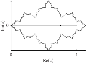
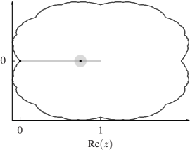
Figure 4: Julia sets for parameters $\mu=-0.65$ (left) and $\mu=-0.2$ (right) for $C_{k}=-\operatorname{id}$. The Julia set of $g_{\mu,4}$ is depicted in dark gray whereas the Julia set of the original map, i.e., the unit interval, is depicted in medium gray. The fixed points ${z^{*}}=0$ and ${z^{*}}=\frac{3}{4}$ are marked by black dots. Shaded circles indicate $B(\varepsilon,{z^{*}})$ for $\mu_{0}=\mu$.

What does stabilization of fixed points mean in terms of complex analytic dynamics? An unstable fixed point is contained in the Julia set. The goal of stabilization is to turn this fixed point into a stable one, i.e., that it now belongs to a bounded Fatou component. That is, the transformation should deform the Julia set in a way that it does not contain the targeted periodic point anymore.

Let us consider the case $r=4$ in more detail. The Julia set $J(\ell_{r=4})=I$ is equal to the whole unit interval. The probability distribution $m$ is given by a beta distribution with parameters both equal to $\frac{1}{2}$ (cf. for example Diakonos1996 ), i.e., with probability density function

$$p(x)=\left(\pi x^{\frac{1}{2}}(1-x)^{\frac{1}{2}}\right)^{-1}.$$

Suppose $C_{k}=\operatorname{id}$ and $\mu$ small enough. In this case ${z^{*}}=\frac{3}{4}$ is the stabilized fixed point. In the previous section we calculated the maximum size of the ball around the fixed point for which the adaptation method works straight away. This radius is given by $\varepsilon<\frac{1}{8}$ and

$$P_{0}=m(V_{0}) \leq m(B(\varepsilon,{z^{*}})\cap I)=m\left(\left[\frac{5}{8},\frac{7}{8}\right]\right)=\int_{\frac{5}{8}}^{\frac{7}{8}}\frac{\mathrm{d}x}{\pi x^{\frac{1}{2}}(1-x)^{\frac{1}{2}}}$$

$$=\frac{2}{\pi}\left(\arctan\left(\sqrt{\frac{3}{5}}\right)-\operatorname{arccot}\left(\sqrt{7}\right)\right)\approx 0.1895.$$

In Figure 4, one can see that the whole unit interval is contained in the bounded Fatou component. Backward iteration takes this set closer to the boundary of this Fatou component. This means that, for $\mu_{0}$ small,

$$\varphi(\mu_{0})=1,$$

$P_{0}\leq P_{k}=m(V_{k})\leq 1$ and $\tilde{\varphi}=1$. Therefore, trajectories will converge to the stabilized periodic point with probability one.

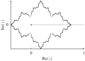
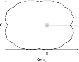
Figure 5: Julia sets for parameters $\mu=-0.65$ (left) and $\mu=-0.2$ (right) for $C_{k}=\operatorname{id}$. The Julia set of $g_{\mu,4}$ is depicted in dark gray whereas the Julia set of the original map, i.e., the unit interval, is depicted in medium gray. The fixed points ${z^{*}}=0$ and ${z^{*}}=\frac{3}{4}$ are marked by black dots. Shaded circles indicate $B(\varepsilon,{z^{*}})$ for $\mu_{0}=\mu$.

The picture is slightly different for $C_{k}=-\operatorname{id}$ and $\mu$ small enough. Now, ${z^{*}}=0$ is the stabilized fixed point. Again we have $\varepsilon<\frac{1}{8}$ and therefore

$$P_{0}=m(V_{0}) \leq m(B(\varepsilon,{z^{*}})\cap I)=m\left(\left[0,\frac{1}{8}\right]\right)=\int_{0}^{\frac{1}{8}}\frac{\mathrm{d}x}{\pi x^{\frac{1}{2}}(1-x)^{\frac{1}{2}}}$$

$$=\frac{2}{\pi}\operatorname{arccot}\left(\sqrt{7}\right)\approx 0.2301.$$

In this case backward iteration yields a different result as can be seen in Figure 5. Part of the set of initial conditions $A$ is in the basin of attraction of infinity and the intersection with the Julia set is exactly the fixed point ${z^{*}}=\frac{3}{4}$. Therefore, the probability to converge with a random initial condition is less than one. Integrating the probability density function gives

$$\varphi(\mu_{0})=\int_{0}^{\frac{3}{4}}\frac{\mathrm{d}x}{\pi x^{\frac{1}{2}}(1-x)^{\frac{1}{2}}}=\frac{2}{3}.$$

Therefore, we have $\tilde{\varphi}=\frac{2}{3}$ and $P_{0}\leq m(V_{k})\leq\frac{2}{3}$. In contrast to the case $C_{k}=\operatorname{id}$ this means that for $C_{k}=\operatorname{id}$ and ${z^{*}}=0$ a trajectory with an initial condition on $I$ distributed according to $m$ will diverge with a probability of one third.

When considering higher periods of such a polynomial map, the Julia sets are more complicated as the degree of the iterated polynomial rises exponentially. The situation changes qualitatively when considering the predictive feedback control dynamics of higher dimensional maps by interpreting them as functions $\mathbb{C}^{n}\to\mathbb{C}^{n}$. In general, the dynamics of holomorphic, higher-dimensional maps is more diverse since even low-dimensional invertible maps give rise to complicated dynamics Hubbard1994 .

V Numerical Results

To compare the speed of the adaptive method (ACC) with the original PFC chaos control in a real world application, we performed numerical simulations for the logistic map $\ell_{4}$. The results for $C_{k}=+\operatorname{id}$, $\mu_{0}\in[0,1]$ and periods one and two are summarized in Figure 6. One can clearly see that for most initial values of the control parameter, the adaptive method yields an increase in convergence speed. The results for $C_{k}=-\operatorname{id}$ and period one are similar but the convergence probability is lower (not shown) in accordance with the results of the previous section, cf. Figure 5. In the case of period $p=2$, the orbits stabilized by negative $\mu$ are the period one orbits, which is reflected in our numerical results (not shown). A non-optimized, ad hoc choice of parameters for the adaptive method of $K=8$ and $L_{0}=0.99$ (independent of the initial condition) were employed in the simulations. The criterion for convergence time $T$ was given by $\left|x_{T}-x_{T-1}\right|\leq 10^{-10}$ but reliability was determined after checking for the correct period.

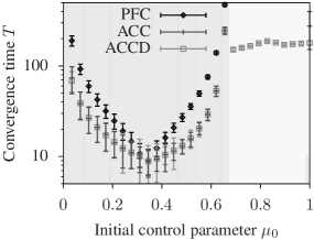
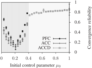
Figure 6: Speed and reliability comparison of the original PFC chaos control ($\mu=\mu_{0}$ fixed) and both ACC and ACCD for the logistic map $\ell_{4}$ with $p=1$ (left) and $p=2$ (right). Times are only plotted if more than $1\%$ of initial values that lead to convergence to the correct period. Gray shading indicate the convergence reliability; dark gray corresponds to all methods converging, light gray to the reliability of ACCD. Convergence time $T$ is given by $\left|x_{T}-x_{T-1}\right|\leq 10^{-10}$ calculated for $1000$ random initial conditions after a transient of random length.

The convergence reliability, i.e., the fraction of trials where the above criterion is fulfilled after some time $T$, is not improved by the adaptive method. However, it is possible to amend the adaptation method to lead to convergence for most initial conditions $x_{0}$ within the convergent regime, independent of the initial value of the control parameter $\mu_{0}$ (the modified method is denoted by ACCD). When adapting, the ACC method has to check whether Criterion (5a) is fulfilled. If this is not the case after $M$ iterations, the modified method simply reduces $\mu$ to a certain fraction $v$. To prevent $\mu$ of becoming too small, we imply a threshold $\theta$ below which $\mu$ cannot decay. Put in other words, the modified method ACCD will automatically decrease $\mu$ towards zero to reach the convergence regime if Inequality (5a) is not satisfied within a given number of steps.

The modified method ACCD behaves like the original ACC method for initial values of $\mu_{0}$ in the convergent regime while leading to convergence outside of it, cf. Figure 6 (here $M=50$, $v=0.7$, $\theta=0.1$ for period $p=1$, and $\theta=0.05$ for period $p=2$). Failure of convergence that is due to the existence of a range of diverging initial conditions, however, will persist, even with the decay. The results are similar for a broad parameter range (e.g., decay rate $v\in[0.65,0.99]$ and decay kick-in time $M\in[10,100]$). For a decay rate too close to $100\%$ or a too large decay kick-in time, it will take many iterations to reach the convergent interval. On the other hand, if the decay kick-in time is too small or does not exist at all, $\mu_{k}$ decreases even if it is in the convergent interval as Criterion (5a) is not fulfilled all the time, unnecessarily increasing convergence time.

VI Discussion

Here we presented a method which adapts the control parameter $\mu$ of the PFC method in order to accelerate the systems convergence to a periodic orbit. In contrast to heuristically chosen methods, our adaptation does not compromise convergence. The algorithm converges in a neighborhood of every periodic orbit that was stabilized by the stabilizing transformation. Assuming the existence of an invariant, ergodic probability measure on the chaotic attractor, we obtain an analytic bound for the probability $P_{k}$ that the system converges to a periodic orbit if the chaos control is switched on at an arbitrary point in time. Although these results are stated in the framework of discrete time dynamical systems, they can also be applied to stabilize continuous time systems after discretization such as taking Poincaré sections. The logistic map provides an example for which we can calculate the parameters for the method. We estimated the probability of convergence and highlighted its dependence on the fixed point to be stabilized and the associated matrix $C_{k}$.

Our method was stated in the general context of “chaotic sets.” In general, such sets do not need to be local or even global attractors of the dynamical system. In fact, the Julia sets considered in the example are repelling rather than attracting. In applications, however, an attractor would be desirable such that the process of stabilization becomes repeatable. That is, after the control perturbation is turned off by choosing the appropriate value for the control parameter, the dynamics would return to the attractor and the process can be started over again.

Apart from its role as a chaos control method, the estimates described in §III.2 give information on the PFC method itself. It allowed us to calculate the size of the basin of attraction for varying $\mu$ in our example. Decreasing $\mu$ always leads to slower convergence since the eigenvalues converge to one as $\mu\to 0$. So is it possible to find an optimal $\mu_{0}$ for a given map? Since any adaptation method increases the computational cost of the chaos control method, a priori estimates of such crucial quantities are of importance. Furthermore, the choice of the stabilization matrix $C_{k}$ depends on the type of fixed points in the chaotic attractor. Hence, global statistics for a given map $f$ of the periodic orbits and their stability properties might yield some a priori estimates.

Our numerical studies suggest that it is possible to get reliable convergence without a priori knowledge of the exact values for the parameters. A slight modification of the method yields a hybrid method that finds the regime of control parameter in which the dynamics converge online and then adapt it to the optimal value. This simplification, however, comes at a cost in convergence speed. By definition, PFC cannot distinguish between a periodic orbit of period $p$ and any $q|p$, a divisor of $p$. Our numerical calculations, however, indicate that this does not influence reliability of the chaos control method. This is most likely caused by the exponential growth of the number of periodic orbits. In the future, it would be desirable to add a mechanism that rigorously distinguishes between the target period and its divisors to prove optimal convergence.

An adaptation method for chaos control is a step towards solving the intuitively contradictory problem of optimizing speed while maintaining simplicity in implementation. However, as discussed above, it leads to further challenging research questions that have to be addressed in the future.

References

- [1] E. Schöll and H. G. Schuster. Handbook of Chaos Control. Wiley-VCH Verlag, Weinheim, Germany, 1999.
- [2] M. I. Rabinovich and H. D. I. Abarbanel. The role of chaos in neural systems. Neuroscience, 87(1):5–14, 1998.
- [3] S. Steingrube, M. Timme, F. Wörgötter, and P. Manoonpong. Self-organized adaptation of a simple neural circuit enables complex robot behaviour. Nat. Phys., 6(3):224–230, 2010.
- [4] E. Schöll. Neural control: Chaos control sets the pace. Nat. Phys., 6(3):161–162, 2010.
- [5] E. Ott, C. Grebogi, and J. A. Yorke. Controlling Chaos. Phys. Rev. Lett., 64(11):1196–1199, 1990.
- [6] M. de Sousa Vieira and A. Lichtenberg. Controlling chaos using nonlinear feedback with delay. Phys. Rev. E, 54(2):1200–1207, 1996.
- [7] B. T. Polyak. Stabilizing Chaos with Predictive Control. Autom. Remote Control, 66(11):1791–1804, 2005.
- [8] P. Schmelcher and F. K. Diakonos. Detecting Unstable Periodic Orbits of Chaotic Dynamical Systems. Phys. Rev. Lett., 78(25):4733–4736, 1997.
- [9] P. Schmelcher and F. K. Diakonos. General approach to the localization of unstable periodic orbits in chaotic dynamical systems. Phys. Rev. E, 57(3):2739–2746, 1998.
- [10] D. Yang and P. Yang. Numerical instabilities and convergence control for convex approximation methods. Nonlinear Dynam., 61(4):605–622, 2010.
- [11] M. E. Brewster and R. Kannan. Nonlinear Successive Over-Relaxation. Numer. Math., 44(2):309–315, 1984.
- [12] F. K. Diakonos, P. Schmelcher, and O. Biham. Systematic Computation of the Least Unstable Periodic Orbits in Chaotic Attractors. Phys. Rev. Lett., 81(20):4349–4352, 1998.
- [13] D. Pingel, P. Schmelcher, F. K. Diakonos, and O. Biham. Theory and applications of the systematic detection of unstable periodic orbits in dynamical systems. Phys. Rev. E, 62(2):2119–34, 2000.
- [14] D. Pingel, P. Schmelcher, and F. K. Diakonos. Stability transformation: a tool to solve nonlinear problems. Phys. Rep., 400(2):67–148, 2004.
- [15] J. J. Crofts and R. L. Davidchack. Efficient Detection of Periodic Orbits in Chaotic Systems by Stabilizing Transformations. SIAM J. Sci. Comput., 28(4):1275, 2006.
- [16] J. J. Crofts and R. L. Davidchack. On the use of stabilizing transformations for detecting unstable periodic orbits in high-dimensional flows. Chaos, 19(3):033138, 2009.
- [17] B. Doyon and L. Dubé. Targeting unknown and unstable periodic orbits. Phys. Rev. E, 65(3):1–4, 2002.
- [18] R. L. Davidchack and Y.-C. Lai. Efficient algorithm for detecting unstable periodic orbits in chaotic systems. Phys. Rev. E, 60(5):6172–6175, 1999.
- [19] J. Lehnert, P. Hövel, V. Flunkert, P. Yu. Guzenko, A. L. Fradkov, and E. Schöll. Adaptive tuning of feedback gain in time-delayed feedback control. Chaos, 21(4):043111, 2011.
- [20] J. Milnor. Dynamics in one complex variable, volume 160 of Annals of Mathematics Studies. Princeton University Press, Princeton, NJ, third edition, 2006.
- [21] A. S. Householder. Minimal Matrix Norms. Monatsh. Math., 63(4):344–350, 1959.
- [22] D. A. Smith, W. F. Ford, and A. Sidi. Extrapolation Methods for Vector Sequences. SIAM Rev., 29(2):199–233, 1987.
- [23] F. K. Diakonos and P. Schmelcher. On the construction of one-dimensional iterative maps from the invariant density: the dynamical route to the beta-distribution. Phys. Lett. A, 211(1):199–203, 1996.
- [24] J. H. Hubbard and R. W. Oberste-Vorth. Hénon mappings in the complex domain I: The global topology of dynamical space. Publ. Math. Inst. Hautes Études Sci., 79(1):5–46, 1994.