Translation representations and scattering by two intervals

Abstract.

Studying unitary one-parameter groups in Hilbert space $(U(t),\mathscr{H})$, we show that a model for obstacle scattering can be built, up to unitary equivalence, with the use of translation representations for $L^{2}$-functions in the complement of two finite and disjoint intervals.

The model encompasses a family of systems $(U(t),\mathscr{H})$. For each, we obtain a detailed spectral representation, and we compute the scattering operator, and scattering matrix. We illustrate our results in the Lax-Phillips model where $(U(t),\mathscr{H})$ represents an acoustic wave equation in an exterior domain; and in quantum tunneling for dynamics of quantum states.

To the memory of William B. Arveson.

1. Introduction

For a number of problems in analysis, one is faced with a unitary one-parameter group acting on a Hilbert space. In such a problem, if an energy form is preserved, this allows one to create a Hilbert space $\mathscr{H}$, and then to study how states change, as a function of time, via a one-parameter group of unitary operators $U(t)$ acting in $\mathscr{H}$. Here $t$ is representing time.

For the study of scattering theory, Lax and Phillips suggested in [LP68] that one looks for two unitarily equivalent versions of $U(t)$. For the acoustic wave equation, for example, with scattering around a finite obstacle, Lax and Phillips proved that, in each of these two representations, the equivalent unitary one-parameter group may be taken to be a “copy of” the group of translations of $L^{2}$-functions on the real line $\mathbb{R}$, but functions taking values in a fixed Hilbert space $\mathscr{M}$. By “a copy” we mean a one-parameter group which in unitarily equivalent to $U(t)$. As a result, one gets two isometric transforms from $\mathscr{H}$ into $L^{2}(\mathbb{R},\mathscr{M})$.

The two representations are called “translation representations;” one incoming, and the other outgoing. It is known that the same idea is applicable to certain instances of dynamics of quantum states governed by a Schrödinger equation. In the Lax-Phillips model, given, as above, a pair $(\mathscr{H},U(t))$, Hilbert space, and unitary one-parameter group, one looks for two closed subspaces $D_{in}$ (incoming states) and $D_{out}$ (outgoing states) in $\mathscr{H}$. Incoming refers to “before the obstacle;” and outgoing, after. On the incoming states $f_{in}$, $U(t)$ acts by translation to the left, so acting before the “obstacle,” while the outgoing states $f_{out}$, $U(t)$ acts by translation to the right. A scattering operator $S$ will act between the two subspaces, $Sf_{in}=f_{out}$, sending $f_{in}$ into $f_{out}$.

A second source of motivation for our analysis of exterior problems derives from recent work on exterior dynamical systems; now extensively studied under the heading “outer billiard,” or dual billiard, or anti-billiard; see e.g., [Sch11, Sch09]. Unlike billiard [Mos08], the “outer” game is played outside of the table (a convex domain). The role of unitary operators in Hilbert space is supported by a theorem of Moser which asserts that the outer billiard map is area-preserving.

Now, in realistic models, detailed properties of an obstacle are often difficult to come by, and it is therefore useful to work through some idealized models for obstacle. In the simplest such models, for example the complement of two bounded disjoint intervals in $\mathbb{R}$, one can rephrase the problem in the language of von Neumann’s deficiency indices, and deficiency subspaces, see [vN32, DS88] and Section 2 below.

This is the focus of our present analysis, and it covers such examples from quantum mechanics as quantum tunneling. Now, as above, fix two bounded intervals $I_{1}$ and $I_{2}$, and let $\Omega$ denote the complement, i.e., $\Omega=\mathbb{R}\backslash(I_{1}\cup I_{2})$. So $\Omega$ has one bounded component, and two unbounded. Since translation of $L^{2}$-functions is generated by the derivative operator $D$, it is natural to study $D$ as a skew-symmetric operator with domain dense in $L^{2}(\Omega)$ consisting of functions $f$ such that $f,Df\in L^{2}(\Omega)$, and $f$ vanishes on the four boundary points. This is called the minimal operator. The corresponding adjoint operator is the maximal one; see Remark 2.4 and [JPT11, DS88].

A degenerate instance of this is when $\Omega$ is instead the complement of 2 points. In both cases, the minimal operator $D$ will have deficiency indices $(2,2)$. Using our analysis from [JPT11], one sees that we then get all the skew-selfadjoint extensions of $D=\frac{d}{dx}$ indexed by the group $U(2)$ of all unitary $2\times 2$ matrices. This can be done such that, for every $B$ in $U(2)$, we realize a corresponding skew-selfadjoint boundary conditions (bc-B), and therefore a unitary one-parameter group $U_{B}(t)$ acting on $L^{2}(\Omega)$. In our paper we find the scattering theory, as well as the spectral theory, of each of these unitary one-parameter groups.

For each $U_{B}(t)$ we find a system of generalized eigenfunctions. They are determined by three functions $a_{B}$, $b_{B}$, and $c_{B}$, one for each of the three connected components of $\Omega$.

1.1. Overview

We undertake a systematic study of interconnections between geometry and spectrum for a family of selfadjoint operator extensions indexed by two things: by (i) the prescribed configuration of the two intervals, and by (ii) the von Neumann parameters (see (1.2)). This turns out to be subtle, and we show in detail how variations in both (i) and (ii) translate into explicit spectral properties for the extension operators. Indeed, for each choice in (i) , i.e., relative length of the two intervals, we have a Hermitian operator with deficiency indices $(2,2).$ Our main theme is spectral theory of the corresponding family of $(2,2)$-selfadjoint extension operators.

In section 2, we introduce some tools, reproducing kernels and von Neumann deficiency indices, for dealing with the main setting: A direct integral representation of the boundary value problem. The selfadjoint realizations correspond to a family of unitary one-parameter groups, each one generated by skew-selfadjoint extension of a minimal first order differential operator in open and unbounded subset $\Omega$ of $\mathbb{R}$.

A key point here is that the unitary one-parameter groups are parametrized by one of the unitary matrix groups $U(n)$. Here, the number $n$ is related to $\Omega$ as follows: $\Omega$ has two unbounded components, and $n-1$ bounded components.

Section 3 contains detailed computations of spectral data for unitary one parameter groups $U_{B}(t)$ acting in $L^{2}(\Omega)$, indexed by $B$ in $U(n)$: An explicit presentation of the generalized eigenfunction direct-integral presentation. The essential points in our analysis are revealed in the case $n=2$, and we therefore present the details for $U(2)$. We show that the measure in the direct integral decomposition of $U_{B}(t)$ is of the form $\sigma_{B}(d\lambda)=P_{B}(\lambda)d\lambda$ with periodic density, and where, in each period-interval, $P_{B}$ is a Poisson kernel depending on $B$ in $U(2)$. We further find that the cases of embedded point-spectrum (Dirac combs) arise as a limit taking place in the group $U(2)$.

Within each section, the results are illustrated with applications from physics and from harmonic analysis.

Sections 4 - 7 deal with scattering theory for the unitary one-parameter groups $U_{B}(t)$. This is presented in terms of time-delay operators, translation representations, and Lax-Phillips scattering operators. Closely connected to the scattering operator is the Lax-Phillips contraction semigroup; it is computed in section 6.

1.2. Unbounded Operators

We recall the following fundamental result of von Neumann on extensions of Hermitian operators.

In order to make precise the boundary form for the cases (2.6) - (2.7) we need a:

Lemma 1.1.

Let $\Omega\subset\mathbb{R}$ be as above. Suppose $f$ and $f^{\prime}=\frac{d}{dx}f$ (distribution derivative) are both in $L^{2}(\Omega)$; then there is a continuous function $\tilde{f}$ on $\overline{\Omega}$ (closure) such that $f=\tilde{f}$ a.e. on $\Omega$, and $\lim_{\left|x\right|\rightarrow\infty}\tilde{f}(x)=0$.

Proof.

Let $p\in\mathbb{R}$ be a boundary point. Then for all $x\in\Omega$, we have:

$$f(x)-f(p)=\int_{p}^{x}f^{\prime}(y)dy.$$ (1.1)

Indeed, $f^{\prime}\in L_{loc}^{1}$ on account of the following Schwarz estimate

$$\left|f(x)-f(p)\right|\leq\sqrt{\left|x-p\right|}\left\|f^{\prime}\right\|_{L^{2}(\Omega)}.$$

Since the RHS in (1.1) is well-defined, this serves to make the LHS also meaningful. Now set

$$\tilde{f}(x):=f(p)+\int_{p}^{x}f^{\prime}(y)dy,$$

and it can readily be checked that $\tilde{f}$ satisfies the conclusions in the Lemma.∎

Lemma 1.2 (see e.g. [DS88]).

Let $L$ be a closed Hermitian operator with dense domain $\mathscr{D}_{0}$ in a Hilbert space. Set

$$\mathscr{D}_{\pm} = \{\psi_{\pm}\in dom(L^{*})\left.\right|L^{*}\psi_{\pm}=\pm i\psi_{\pm}\}$$

$$\mathscr{C}(L) = \{U:\mathscr{D}_{+}\rightarrow\mathscr{D}_{-}\left.\right|U^{*}U=P_{\mathscr{D}_{+}},UU^{*}=P_{\mathscr{D}_{-}}\}$$ (1.2)

where $P_{\mathscr{D}_{\pm}}$ denote the respective projections. Set

$$\mathscr{E}(L)=\{S\left.\right|L\subseteq S,S^{*}=S\}.$$

Then there is a bijective correspondence between $\mathscr{C}(L)$ and $\mathscr{E}(L)$, given as follows:

If $U\in\mathscr{C}(L)$, and let $L_{U}$ be the restriction of $L^{*}$ to

$$\{\varphi_{0}+f_{+}+Uf_{+}\left.\right|\varphi_{0}\in\mathscr{D}_{0},f_{+}\in\mathscr{D}_{+}\}.$$ (1.3)

Then $L_{U}\in\mathscr{E}(L)$, and conversely every $S\in\mathscr{E}(L)$ has the form $L_{U}$ for some $U\in\mathscr{C}(L)$. With $S\in\mathscr{E}(L)$, take

$$U:=(S-iI)(S+iI)^{-1}\left.\right|_{\mathscr{D}_{+}}$$ (1.4)

and note that

1. $U\in\mathscr{C}(L)$, and

2. $S=L_{U}$.

Vectors $f$ in $dom(L^{*})$ admit a unique decomposition $f=\varphi_{0}+f_{+}+f_{-}$ where $\varphi_{0}\in dom(L)$, and $f_{\pm}\in\mathscr{D}_{\pm}$. For the boundary-form $\mathbf{B}(\cdot,\cdot)$, we have

$$i\mathbf{B}(f,f) = \left\langle L^{*}f,f\right\rangle-\left\langle f,L^{*}f\right\rangle$$

$$= \left\|f_{+}\right\|^{2}-\left\|f_{-}\right\|^{2}.$$

1.3. Prior Literature

There are related investigations in the literature on spectrum and deficiency indices. For the case of indices $(1,1)$, see for example [ST10, Mar11]. For a study of odd-order operators, see [BH08]. Operators of even order in a single interval are studied in [Oro05]. The paper [BV05] studies matching interface conditions in connection with deficiency indices $(m,m)$. Dirac operators are studied in [Sak97]. For the theory of selfadjoint extensions operators, and their spectra, see [Šmu74, Gil72], for the theory; and [Naz08, VGT08, Vas07, Sad06, Mik04, Min04] for recent papers with applications. For applications to other problems in physics, see e.g., [AHM11, PR76, Bar49, MK08]. For related problems regarding spectral resolutions, but for fractal measures, see e.g., [DJ07, DHJ09, DJ11].

2. Momentum Operators

By momentum operator $P$ we mean the generator for the group of translations in $L^{2}(-\infty,\infty)$, see (2.4) below. There are several reasons for taking a closer look at restrictions of the operator $P.$ In our analysis, we study spectral theory determined by the complement of two bounded disjoint intervals, i.e., the union of one bounded component and two unbounded components (details below.) Our motivation derives from quantum theory (see section 5), and from the study of spectral pairs in geometric analysis; see e.g., [DJ07], [Fug74], [JP99], [Łab01], and [PW01]. In our model, we examine how the spectral theory depends on both variations in the choice of the two intervals, as well as on variations in the von Neumann parameters.

Granted that in many applications, one is faced with vastly more complicated data and operators; nonetheless, it is often the case that the more subtle situations will be unitarily equivalent to a suitable model involving $P$. This is reflected for example in the conclusion of the Stone-von Neumann uniqueness theorem: The Weyl relations for quantum systems with a finite number of degree of freedom are unitarily equivalent to the standard model with momentum and position operators $P$ and $Q$. For details, see e.g., [Jør81].

2.1. The boundary form, spectrum, and the group $U(2)$

Since the problem is essentially invariant under affine transformations we may assume the two intervals are $I_{1}=[0,1]$ and $I_{2}=[\alpha,\beta]$, $\alpha>1$; and the exterior domain

$$\Omega:=I_{-}\cup I_{0}\cup I_{+}$$ (2.1)

consists of three components

$$I_{-}:=(-\infty,0),\>I_{0}:=(1,\alpha),\>I_{+}:=(\beta,\infty).$$ (2.2)

Let $L^{2}(\Omega)$ be the Hilbert space with respect to the inner product

$$\langle f\mid g\rangle:=\int_{I_{-}}f\overline{g}+\int_{I_{0}}f\overline{g}+\int_{I_{+}}f\overline{g}$$ (2.3)

The maximal momentum operator is

$$P:=\frac{1}{i2\pi}\frac{d}{dt}$$ (2.4)

with domain $\mathscr{D}(P)$ equal to the set of absolutely continuous functions on $\Omega$ where both $f$ and $Pf$ are square-integrable.

The boundary form associated with $P$ is defined as the form

$$\mathbf{B}(f,g):=\langle Pf\mid g\rangle-\langle f\mid Pg\rangle$$ (2.5)

on $\mathscr{D}(P).$ Clearly,

$$\mathbf{B}(f,g)=f(1)\overline{g(1)}-f(0)\overline{g(0)}+f(\beta)\overline{g(\beta)}-f(\alpha)\overline{g(\alpha)}.$$ (2.6)

For $f\in\mathscr{D}\left(P\right),$ let $\rho_{1}(f):=\left(f(1),f(\beta)\right)$ and $\rho_{2}(f):=\left(f(0),f(\alpha)\right).$ Then

$$\mathbf{B}(f,g)=\left\langle\rho_{1}(f)\mid\rho_{1}(g)\right\rangle-\left\langle\rho_{2}(f)\mid\rho_{2}(g)\right\rangle.$$ (2.7)

Hence $\left(\mathbb{C}^{2},\rho_{1},\rho_{2}\right)$ is a boundary triple for $P.$ The set of selfadjoint restrictions of $P$ is parametrized by the group $U(2)$ of all unitary $2\times 2$ matrices, see e.g., [dO09]. Explicitly, any unitary $2\times 2$ matrix $B$ determines a selfadjoint restriction $P_{B}$ of $P$ by setting

$$\mathscr{D}\left(P_{B}\right):=\left\{f\in\mathscr{D}\left(P\right)\mid B\rho_{1}(f)=\rho_{2}(f)\right\}.$$ (2.8)

Conversely, every selfadjoint restriction of $P$ is obtained in this manner.

When $B\in U(2)$ is fixed, we will denote the corresponding selfadjoint extension operator $P_{B}$. (For our parametrization of $U(2)$ see (2.21).)

In sections 2 and 3 below we prove the following theorem.

Theorem 2.1.

If $B\in U(2)$ has its parameter $w$ satisfying $0<w\leq 1$, then there is a system of bounded generalized eigenfunctions $\{\psi_{\lambda}^{(B)};\lambda\in\mathbb{R}\}$, and a positive Borel function $F_{B}(\cdot)$ on $\mathbb{R}$ such that the unitary one-parameter group $U_{B}(t)$ in $L^{2}(\Omega)$ generated by $P_{B}$ has the form

$$\left(U_{B}(t)f\right)(x)=\int_{\mathbb{R}}e_{\lambda}(-t)\left\langle\psi_{\lambda}^{(B)},f\right\rangle_{\Omega}\psi_{\lambda}^{(B)}(x)F_{B}(\lambda)d\lambda$$ (2.9)

for all $f\in L^{2}(\Omega)$, $x\in\Omega$, and $t\in\mathbb{R}$; where

$$\left\langle\psi_{\lambda}^{(B)},f\right\rangle_{\Omega}:=\int_{\Omega}\overline{\psi_{\lambda}^{(B)}(y)}f(y)dy.$$

We further show that (when $w(B)>0$) the density function $F_{B}(\cdot)$ in (2.9) is periodic in $\lambda$, and that, in each period, $F_{B}(\cdot)$ is a Poisson kernel, determined from a specific action of the group $U(2)$.

In section 2, we prepare with some technical lemmas; and in section 3 we compute explicit formulas for the expansion (2.9) above, and we discuss their physical significance.

In particular, we note that when $w>0$, there are no bound-state contributions to the expansion (2.9). By contrast if $w=0$, there are bound-states. This entails embedded point-spectrum. In all cases the point-spectrum has the form $\frac{1}{l}\mathbb{Z}$ where $l=\alpha-1$ is the length of the interval $I_{0}$.

2.2. Reproducing Kernel Hilbert Space

In this section we introduce a certain reproducing kernel Hilbert space $\mathscr{H}_{1}(\Omega)$; a first order Sobolev space, hence the subscript 1. Its reproducing kernel is found (Lemma 2.2), and it serves two purposes: First, we show that each of the unbounded selfadjoint extension operators $P_{B}$, defined from (2.8) in sect 2.1, have their graphs naturally embedded in $\mathscr{H}_{1}(\Omega)$. Secondly, for each $P_{B}$, the reproducing kernel for $\mathscr{H}_{1}(\Omega)$ helps us pin down the generalized eigenfunctions for $P_{B}$. The arguments for this are based in turn on Lemma 1.2 and the boundary form $\boldsymbol{B}$ from (2.5) and (2.6).

Lemma 2.2.

Let

$$\Omega=I_{-}\cup I_{0}\cup I_{+}$$ (2.10)

be as above, and $L^{2}(\Omega)$ be the Hilbert space of all $L^{2}$-functions on $\Omega$ with inner product $\left\langle\cdot,\cdot\right\rangle_{\Omega}$ and norm $\left\|\cdot\right\|_{\Omega}$. Set

$$\mathscr{H}_{1}(\Omega)=\{f\in L^{2}(\Omega)\left|\right.Df=f^{\prime}\in L^{2}(\Omega)\};$$

then $\mathscr{H}_{1}(\Omega)$ is a reproducing kernel Hilbert space of functions on $\overline{\Omega}$ (closure).

Proof.

For the special case where $\Omega=\mathbb{R}$, the details are in [Jør81]. For the case where $\Omega$ is the exterior domain from (2.10), we already noted (Lemma 1.1) that each $f\in\mathscr{H}_{1}(\Omega)$ has a continuous representation $\tilde{f}$, and that $\tilde{f}$ vanishes at $\pm\infty$. The inner product in $\mathscr{H}_{1}(\Omega)$ is

$$\left\langle f,g\right\rangle_{\mathscr{H}_{1}(\Omega)}=\left\langle f,g\right\rangle_{\Omega}+\left\langle f^{\prime},g^{\prime}\right\rangle_{\Omega}.$$ (2.11)

Let $x\in\overline{\Omega}=\overline{I}_{-}\cup\overline{I}_{0}\cup\overline{I}_{+}$, and denote by $J$ the interval containing $x;$ and let $p$ be a boundary point in $J$. Then an application of Cauchy-Schwarz yields

$$\left|\tilde{f}(x)\right|^{2}-\left|\tilde{f}(p)\right|^{2} =2\Re\int_{p}^{x}\overline{f(y)}f^{\prime}(y)dy$$

$$\leq\left\|f\right\|_{J}^{2}+\left\|f^{\prime}\right\|_{J}^{2}\leq\left\|f\right\|_{\mathscr{H}_{1}(\Omega)}^{2}.$$

We conclude that the linear functional

$$\mathscr{H}_{1}(\Omega)\ni f\rightsquigarrow\tilde{f}(x)\in\mathbb{C}$$

is continuous on $\mathscr{H}_{1}(\Omega)$ with respect to the norm from (2.11). By Riesz, applied to $\mathscr{H}_{1}(\Omega)$, we conclude that there is a unique $k_{x}\in\mathscr{H}_{1}(\Omega)$ such that

$$\tilde{f}(x)=\left\langle k_{x},f\right\rangle_{\mathscr{H}_{1}(\Omega)}$$ (2.12)

for all $f\in\mathscr{H}_{1}(\Omega)$.

If $x$ in (2.12) is a boundary point, then the formula must be modified using instead $\tilde{f}(x_{+})=$ limit from the right if $x$ is a left-hand side end-point in $J$. If $x$ is instead a right-hand side end-point in $J$, then use $\tilde{f}(x_{-})$ in formula (2.12). This concludes the proof of the Lemma. ∎

We are using here standard tools on reproducing kernel Hilbert spaces (RKHS). For the essential properties of RKHSs, and their use in scattering theory, see [ASV06, ADR02].

Lemma 2.3.

Let $\Omega\subset\mathbb{R}$ be an open subset, and let $J=(a,b)$ be a bounded connected component in $\Omega$. Then the reproducing kernels for evaluation in $\mathscr{H}_{1}(\Omega)$ at the two endpoints $a$ and $b$ depend only on $\mathscr{H}_{1}(J)$. The two kernels $k_{a}$ and $k_{b}$ can be taken to be zero in $\Omega\backslash J$. Let

$$k_{a}(x)=\frac{\mbox{coh}(b-x)}{\mbox{sih}(b-a)}$$ (2.13)

and

$$k_{b}(x)=\frac{\mbox{coh}(x-a)}{\mbox{sih}(b-a)}$$ (2.14)

defined for all $x\in J$, and $0$ in $\Omega\backslash J$. Here, coh, and sih denote the usual hyperbolic trigonometric functions. Then

$$\tilde{f}(a_{+})=\left\langle k_{a},f\right\rangle_{\mathscr{H}_{1}(\Omega)},\>\mbox{and }\tilde{f}(b_{-})=\left\langle k_{b},f\right\rangle_{\mathscr{H}_{1}(\Omega)}$$ (2.15)

hold for all $f\in\mathscr{H}_{1}(\Omega)$.

For $a<x<b$, the reproducing kernel function $k_{x}(\cdot)$ of

$$f(x)=\left\langle k_{x},f\right\rangle_{\mathscr{H}_{1}(\Omega)},\>f\in\mathscr{H}_{1}(\Omega)$$ (2.16)

is

$$k_{x}(y)=\frac{\mbox{sih}(b-x)\mbox{coh}(b-y)+\mbox{sih}(x-a)\mbox{coh}(y-a)}{\left(\mbox{sih}(b-a)\right)^{2}}.$$ (2.17)

Proof.

Since the two kernels are zero in the complement $\Omega\backslash J$, we only need to determine them in the interval $J=(a,b)$. A direct analysis shows that they must have the form

$$Ae^{a-x}+Be^{x-b}$$ (2.18)

where $A$ and $B$ are constants to be determined from the two conditions (2.15). When this is done we find the values of $A$ and $B$ in (2.18), and a computation yields the desired formulas (2.13) and (2.14). The formula (2.17) for the kernel function $k_{x}$, when $x$ is an interior point, may be obtained from the endpoint formulas (2.13) and (2.14), and an interpolation argument.∎

Remark 2.4.

Consider the operator $P_{min}$ in $L^{2}(\Omega)$ with domain

$$\mathscr{D}(P_{min})=\{f\in\mathscr{H}_{1}(\Omega);\tilde{f}\equiv 0\mbox{ on }\partial\Omega\},$$ (2.19)

and $P_{min}=\frac{1}{i2\pi}\frac{d}{dx}$. Then $P_{min}$ is Hermitian (symmetric) on its domain in $L^{2}(\Omega)$, and for its adjoint operator $P_{min}^{*}$ we have $\mathscr{D}(P_{min}^{*})=\mathscr{H}_{1}(\Omega)$. Moreover, for every $B\in U(2)$, we have two strict inclusions of graphs:

$$P_{min}\subsetneqq P_{B}\subsetneqq P_{min}^{*}(=P_{max}).$$ (2.20)

Remark 2.5.

The connection between the boundary form formulation and the von Neumann deficiency space approach is further explored in [JPT11].

The family of unitary $2\times 2$ matrices is parameterized by

$$B=\left(\begin{array}[]{cc}w\>e(\phi)&-\sqrt{1-w^{2}}\>e(\theta-\psi)\\ \sqrt{1-w^{2}}\>e(\psi)&w\>e(\theta-\phi)\end{array}\right)$$ (2.21)

where $0\leq w\leq 1$, $\theta,\phi,\psi\in\mathbb{R}$, and

$$e(x):=e^{i2\pi x}.$$ (2.22)

From (2.21), note $\det B=e(\theta)$; and (2.21) is consistent with the parametrization of $SU_{2}$ as follows:

$$\left(\begin{array}[]{cc}\overline{a}&-b\\ \overline{b}&a\end{array}\right)$$ (2.23)

where $a,b\in\mathbb{C}$ satisfy $\left|a\right|^{2}+\left|b\right|^{2}=1$. We have $a=w\>e(-\phi)$, and so $w=\left|a\right|\in[0,1]$.

Proposition 2.6.

Let $\alpha,\beta\in\mathbb{R}$, $1<\alpha<\beta<\infty$, and set

$$\Omega=(-\infty,0)\cup(1,\alpha)\cup(\beta,\infty)$$ (2.24)

be as in (2.28)-(2.2). Let $B\in U(2)$, and let $P_{B}$ be the corresponding selfadjoint operator (see Lemma 1.2). Let $k_{0}$, $k_{1}$, $k_{\alpha}$, and $k_{\beta}$ be the reproducing kernels of the four boundary points in (2.24), see Lemma 2.2. Set

$$k_{R}=\left(\begin{array}[]{c}k_{0}\\ k_{\alpha}\end{array}\right)\mbox{ and \,\ }k_{L}=\left(\begin{array}[]{c}k_{1}\\ k_{\beta}\end{array}\right)$$ (2.25)

as elements in $\mathscr{H}_{1}(\Omega)\oplus\mathscr{H}_{1}(\Omega)$, $L$ for points on the left, and $R$ for right-hand side boundary points. Then $P_{B}$ is characterized by its dense domain in $L^{2}(\Omega)$ as follows:

$$\mathscr{D}(P_{B})=\left\{f\in\mathscr{H}_{1}(\Omega);f\oplus f\perp\left(k_{R}-Bk_{L}\right)\mbox{ in }\mathscr{H}_{1}(\Omega)\oplus\mathscr{H}_{1}(\Omega)\right\}.$$ (2.26)

Proof.

The graph of $P_{B}$ is

$$G(P_{B})=\left\{\left(\begin{array}[]{c}f\\ P_{B}f\end{array}\right);f\in\mathscr{D}(P_{B})\right\},$$

see (2.8), and

$$\left\|f\right\|_{L^{2}(\Omega)}^{2}+\left\|P_{B}f\right\|_{L^{2}(\Omega)}^{2}=\left\|f\right\|_{\mathscr{H}_{1}(\Omega)}^{2},\>f\in\mathscr{D}(P_{B}).$$

Hence the characterization of $\mathscr{D}(P_{B})$ in (2.8) reads:

$$B\left(\begin{array}[]{c}\left\langle k_{1},f\right\rangle_{\mathscr{H}_{1}(\Omega)}\\ \left\langle k_{\beta},f\right\rangle_{\mathscr{H}_{1}(\Omega)}\end{array}\right)=\left(\begin{array}[]{c}\left\langle k_{0},f\right\rangle_{\mathscr{H}_{1}(\Omega)}\\ \left\langle k_{\alpha},f\right\rangle_{\mathscr{H}_{1}(\Omega)}\end{array}\right),\>f\in\mathscr{D}(P_{B}),$$ (2.27)

where we have used Lemma 2.2. Introducing $k_{L}$ and $k_{R}$ as in (2.25), we see that (2.27) is indeed equivalent to the characterization in (2.26).∎

Remark 2.7.

The characterization (2.26) in Proposition 2.6 extends to more general open subsets $\Omega$ in $\mathbb{R}$: It holds mutatis mutandis, that if $\Omega$ is the union of a finite number of bounded components, and two unbounded, i.e.,

$$\Omega=(-\infty,\beta_{1})\cup\bigcup_{i=1}^{n-1}(\alpha_{i},\beta_{i+1})\cup(\alpha_{n},\infty)$$ (2.28)

where

$$-\infty<\beta_{1}<\alpha_{1}<\beta_{2}<\alpha_{2}<\cdots<\alpha_{n-1}<\beta_{n}<\alpha_{n}<\infty.$$

Set

$$k_{R}=\left(\begin{array}[]{c}k_{\beta_{1}}\\ k_{\beta_{2}}\\ \vdots\\ k_{\beta_{n}}\end{array}\right)\;\mbox{and }\>k_{L}=\left(\begin{array}[]{c}k_{\alpha_{1}}\\ k_{\alpha_{2}}\\ \vdots\\ k_{\alpha_{n}}\end{array}\right)$$

in $\bigoplus_{i=1}^{n}\mathscr{H}_{1}(\Omega)$. Let $B$ be a unitary complex $n\times n$ matrix, i.e., $B\in U(n)$; then there is a unique selfadjoint operator $P_{B}$ with dense domain $\mathscr{D}(P_{B})$ in $L^{2}(\Omega)$ such that

$$\mathscr{D}(P_{B})=\left\{f\in\mathscr{H}_{1}(\Omega);\underset{n\mbox{ times}}{\underbrace{f\oplus\cdots\oplus f}}\perp(k_{R}-Bk_{L})\mbox{ in }\bigoplus_{i=1}^{n}\mathscr{H}_{1}(\Omega)\right\};$$ (2.29)

and all the selfadjoint extensions of the minimal operator $D_{min}$ in $L^{2}(\Omega)$ arise this way. In particular, the deficiency indices are $(n,n)$.

Figure 2.1. $\Omega=$ the complement in $\mathbb{R}$ of $n$ finite and disjoint intervals.

Proposition 2.8.

Let $n>2$; and set $J_{i}=(\alpha_{i},\beta_{i+1})$, $J_{-}=(-\infty,\beta_{1})$, $J_{+}=(\alpha_{n},\infty)$ as in (2.28). Set $\tilde{\Omega}=\cup_{i=1}^{n-1}J_{i}$, so

$$L^{2}(\Omega)\cong L^{2}(\tilde{\Omega})\oplus L^{2}(J_{-}\cup J_{+}).$$ (2.30)

Of the selfadjoint extension operators $P_{B}$, indexed by $B\in U(n)$, we get the $\oplus$ direct decomposition

$$P_{B}\cong P_{\tilde{\Omega}}\oplus P_{ext}$$ (2.31)

where $P_{\tilde{\Omega}}$ is densely defined and s.a. in $L^{2}(\tilde{\Omega})$ and $P_{ext}$ is densely defined and s.a. in $L^{2}(J_{-}\cup J_{+})$, if and only if $B$ (in $U(n)$) has the form

$$\left(\begin{array}[]{ccccc}0&\cdots&0&\vline&e(\theta)\\ \hline\cr&&&\vline&0\\ &\huge\mbox{$\tilde{B}$}&&\vline&\vdots\\ &&&\vline&0\end{array}\right)$$ (2.32)

for some $\theta\in\mathbb{R}/\mathbb{Z}$, and $\tilde{B}\in U(n-1)$.

Proof.

Note that presentation (2.32) for some $B\in U(n)$ implies the boundary condition $f(\beta_{n})=e(\theta)f(\alpha_{1})$ for $f\in\mathscr{D}(P_{B})$ when $P_{B}$ is the selfadjoint operator in $L^{2}(\Omega)$ determined in Remark 2.7. And, moreover, the $\oplus$ sum decomposition (2.31) will be satisfied.

One checks that the converse holds as well; see also Theorem 3.8 below; which is a special case.∎

Remark 2.9 (Internal domains vs external).

It is of interest to compare spectral theory for the selfadjoint restrictions $P_{B}$ of the momentum operator in $L^{2}(\Omega)$ in the two cases when $\Omega$ is internal, as opposed to external. By $\Omega$ internal we mean that $\Omega$ is a finite union of disjoint and finite intervals. The case when $\Omega$ is the union of two finite disjoint intervals was considered in [JPT11], and we found that the possibilities for the spectral representation of $P_{B}$ includes both continuous and discrete; but more importantly, we found in [JPT11] that the embedded point-spectrum of some of the selfadjoint operators $P_{B}$ arising this way may be non-periodic.

Contrast this with the external case studied here, i.e., when $\Omega$ is instead the complement of two finite disjoint closed intervals; so the case when $\Omega$ is the union of three components, one bounded $I_{0},$ and two unbounded. There are some aspects of this external problem that are simpler: In the present external problem, the only possibility for point-spectrum is periodic (see Corollary 3.30). The reason for this is that point-spectrum corresponds to bound-states for wave functions trapped in a single bounded interval. In other words, there are only those bound-states that are trapped in the single finite component (see Figure 3.1.) Note in Fig 3.1 the two thick walls (barriers) on either side of $I_{0}$, and the corresponding periodic motion inside $I_{0}$.

Had we instead taken $\Omega$ to be the complement of three finite disjoint closed intervals, then the von Neumann deficiency indices would be $(3,3)$ and there would be examples of $B$ in $U(3)$ such that $P_{B}$ could have non-periodic embedded point-spectrum; so cases analogous to the non-periodic case in [JPT11]. And as a result, the spectral density measure $\sigma_{B}(\cdot)$ might be non-periodic.

3. Spectral Theory

In this section, we fix an exterior domain $\Omega$, the complement of two finite disjoint intervals. For every $B$ in $U(2)$, we introduce the corresponding selfadjoint operator $P_{B}$ with dense domain in $L^{2}(\Omega)$, see (2.8). We are concerned about spectral theory for $P_{B}$, and scattering theory for the unitary one-parameter group $U_{B}(t)$ generated by $P_{B}$. In our study of spectral theory for $\{U_{B}(t)\}_{t\in\mathbb{R}}$, we rely on tools from [Sto90]. In Theorem 3.25 below we show that, for the general case of $B$, $U_{B}(t)$ has simple spectrum (i.e., multiplicity one). Simple spectrum was introduced in [Sto90]. For fixed $B$, we further write down the spectral representation for $U_{B}(t)$.

Our spectral representation formula for $P_{B}$ is presented in Theorem 3.25 below; and the scattering operator (and scattering matrix) for $U_{B}(t)$ is given in Theorem 5.5.

Fix two intervals $I_{1}=[0,1]$ and $I_{2}=[\alpha,\beta]$, $\alpha>1$, and $\Omega=I_{-}\cup I_{0}\cup I_{+}$ being the exterior domain in (3.25), where $I_{-}=(-\infty,0)$, $I_{0}=(1,\alpha)$, and $I_{+}=(\beta,\infty)$. Let $\chi_{-}$, $\chi_{0}$, $\chi_{+}$ be the corresponding characteristic functions.

There is a one-to-one correspondence between selfadjoint restrictions $P_{B}$ of the maximal momentum operator $P$ in $L^{2}(\Omega)$, and the $2\times 2$ unitary matrices $B$ parameterized via (2.21).

The two extreme cases $w=0$, and $w=1$ will be considered separately, i.e.,

$$w=0\>:\; \left(\begin{array}[]{cc}0&-e(\theta-\psi)\\ e(\psi)&0\end{array}\right)$$ (3.3)

$$w=1\>:\; \left(\begin{array}[]{cc}e(\phi)&0\\ 0&e(\theta-\phi)\end{array}\right)$$ (3.6)

We use (2.21) in the computation of the spectrum of the family of selfadjoint operators $P_{B}$ from Section 1.

We show that $w=0$ is a singularity, and gives rise to embedded point-spectrum

$$pt_{spectrum}(P_{B(w=0,\phi,\psi,\theta)})=\frac{\psi}{\alpha-1}+\frac{1}{\alpha-1}\mathbb{Z}$$ (3.7)

embedded in the continuum. (The subscript in (3.7) refers to the degenerate matrix (3.3).) For details, we refer to Theorem 3.8, Figure 3.1, and Remark 3.9 below.

3.1. Spectrum and Eigenfunctions

Fix a unitary $2\times 2$ matrix $B.$

Since the selfadjoint operator has continuous spectrum, possibly with embedded point-atoms, its spectral representation must entail generalized eigenfunctions $\psi_{\lambda}^{(B)}$ with $\lambda\in\mathbb{R}$ denoting the spectral-variable. The reason for “generalized” is that, when $\lambda$ is fixed, $\psi_{\lambda}^{(B)}$ is “trying” to be an eigenfunction, but it is not in $L^{2}(\Omega)$. Hence to make precise the spectral resolution of $P_{B}$ we will need some Gelfand-Schwartz distribution theory.

Let $\mathscr{D}_{B}$ be the $\mbox{$\mathscr{D}$}=C_{c}^{\infty}$ functions on the real line that together with all their derivatives satisfies the boundary condition $B\rho_{1}(\cdot)=\rho_{2}(\cdot).$ Let $\mathscr{D}_{B}\left(\Omega\right)$ be the restrictions of the functions in $\mathscr{D}_{B}$ to $\Omega.$ Since $\mathscr{D}$ and $C_{c}^{\infty}\left(\mathbb{R}\setminus\Omega\right)$ are nuclear and subspaces and quotients of nuclear spaces are nuclear, it follows that $\mathscr{D}_{B}\left(\Omega\right)$ is nuclear.

Let $\dot{P}_{B}$ denote the restriction of $P_{B}$ to $\mathscr{D}_{B}\left(\Omega\right),$ then $\dot{P}_{B}$ is continuous $\mathscr{D}_{B}\left(\Omega\right)\to\mathscr{D}_{B}\left(\Omega\right)$. Let $\mathscr{D}_{B}^{\prime}\left(\Omega\right)$ denote the set of anti-linear continuous functionals on $\mathscr{D}_{B}\left(\Omega\right).$ Then $\dot{P}_{B}$ extends by duality to an operator $\dot{P}_{B}^{\prime}$ on $\mathscr{D}_{B}^{\prime}\left(\Omega\right).$ The duality formula for extending $\dot{P}_{B}$ to $\mathscr{D}_{B}^{\prime}\left(\Omega\right)$ is $\left(\dot{P}_{B}^{\prime}\psi\right)\left(\phi\right)=\psi\left(\dot{P}_{B}\phi\right),$ sometimes we will write this as $\left\langle\phi\left|\dot{P}_{B}^{\prime}\psi\right.\right\rangle=\left\langle\left.\dot{P}_{B}\phi\right|\psi\right\rangle,$ for all $\phi$ in $\mathscr{D}_{B}\left(\Omega\right)$ and all $\psi$ in $\mathscr{D}_{B}^{\prime}\left(\Omega\right).$

A generalized eigenvalue of $P_{B}$ is a real scalar $\lambda$ for which there is a corresponding generalized eigenvector, i.e., a $\psi_{\lambda}$ in $\mathscr{D}_{B}^{\prime}\left(\Omega\right)$ such that

$$\left\langle\phi\left|\dot{P}_{B}^{\prime}\psi_{\lambda}\right.\right\rangle=\lambda\left\langle\phi\mid\psi\right\rangle$$ (3.8)

for all $\phi$ in $\mathscr{D}_{B}\left(\Omega\right).$ Hence the generalized eigenvalues/eigenvectors of $P_{B}$ are ordinary eigenvalues/eigenvectors of $\dot{P}_{B}^{\prime}.$

The following lemmas establish that the spectrum of $P_{B}$ is the real line and that for fixed $\lambda$ the corresponding generalized eigenspace is spanned by the functions

$$\psi_{\lambda}:=\left(a_{\lambda}\chi_{-}+b_{\lambda}\chi_{0}+c_{\lambda}\chi_{+}\right)e_{\lambda}$$ (3.9)

where $a_{\lambda},b_{\lambda},c_{\lambda}$ are scalars such that (2.8) holds, i.e., $B\rho_{1}(\psi_{\lambda})=\rho_{2}(\psi_{\lambda}).$ Recall, $e_{\lambda}(x)=e(\lambda x)=e^{i2\pi\lambda x},$ so we write (3.9) as

$$\psi_{\lambda}(x)=\left(a_{\lambda}\chi_{-}(x)+b_{\lambda}\chi_{0}(x)+c_{\lambda}\chi_{+}(x)\right)e_{\lambda}(x)$$

for $\lambda,x\in\mathbb{R}.$

Lemma 3.1.

Each real number $\lambda$ is a generalized eigenvalue of $P_{B}$ and the corresponding generalized eigenfunctions are the functions (3.9).

Proof.

We can write (3.8) as $\psi_{\lambda}^{\prime}=i2\pi\lambda\psi_{\lambda}.$ Solving this differential equation using weak solution are also strong solutions we see that (3.9) holds. It follows from (3.9) that both sides of (3.8) are given by integrals, hence we can rewrite (3.8) as

$$\int_{\Omega}\phi(t)\,\left(\dot{P}_{B}^{\prime}\psi_{\lambda}\right)(x)\,dx=\int_{\Omega}\left(\dot{P}_{B}\phi\right)(x)\,\psi_{\lambda}(x)\,dx,$$

where $\lambda\in\mathbb{R}$ and $\phi\in\mathscr{D}_{B}\left(\Omega\right).$ Integration by parts, then shows that the boundary form

$$B(\phi,\psi_{\lambda})=\phi(1)\overline{\psi_{\lambda}(1)}-\phi(0)\overline{\psi_{\lambda}(0)}+\phi(\beta)\overline{\psi_{\lambda}(\beta)}-\phi(\alpha)\overline{\psi_{\lambda}(\alpha)}=0,$$

for all $\lambda\in\mathbb{R}$ and all $\phi\in\mathscr{D}_{B}\left(\Omega\right).$ Fixing $\lambda$ and using $\phi$ in $\mathscr{D}_{B}\left(\Omega\right)$ is arbitrary, it follows that $\psi_{\lambda}$ satisfies the boundary condition $B\rho_{1}(\cdot)=\rho_{2}(\cdot).$ ∎

The boundary condition (2.8) gives

$$wb\>e(\phi+\lambda)-\sqrt{1-w^{2}}c\>e(\theta-\psi+\beta\lambda) =a$$ (3.10)

$$\sqrt{1-w^{2}}b\>e(\psi+\lambda)+wc\>e(\theta-\phi+\beta\lambda) =b\>e(\alpha\lambda)$$ (3.11)

Lemma 3.2.

If $0<w\leq 1,$ then each generalized eigenvalue has multiplicity one, and the two functions $\lambda\mapsto a_{B}(\lambda)$ and $\lambda\mapsto c_{B}(\lambda)$ are given by the following formulas:

$$a_{\lambda}=b_{\lambda}w^{-1}e(\phi)e(\lambda)\left(1-\sqrt{1-w^{2}}e(-\psi+(\alpha-1)\lambda)\right)$$ (3.12)

and

$$c_{\lambda}=b_{\lambda}w^{-1}e(\phi-\theta)e(-(\beta-\alpha)\lambda)\left(1-\sqrt{1-w^{2}}e(\psi-(\alpha-1)\lambda)\right).$$ (3.13)

Proof.

If $b=0,$ then (3.10) and (3.11) shows that $a=c=0.$ If $b=1$ we can solve (3.10) and (3.11) for $a$ and $c$. If we assume $b=1$, we can re-write the boundary conditions as

$$w\>e(\phi+\lambda)-\sqrt{1-w^{2}}c_{\lambda}\>e(\theta-\psi+\beta\lambda) =a_{\lambda}$$ (3.14)

$$\sqrt{1-w^{2}}e(\psi+\lambda)+w\>c_{\lambda}\>e(\theta-\phi+\beta\lambda) =e(\alpha\lambda).$$ (3.15)

From (3.15),

$$c_{\lambda}=\frac{e(\alpha\lambda)-\sqrt{1-w^{2}}e(\psi+\lambda)}{we(\theta-\phi+\beta\lambda)}$$ (3.16)

which can be written as 3.12). Substituting (3.16) into (3.15), we get (3.13). ∎

Lemma 3.3.

If $w=0$ then each point $\lambda\in-\frac{\psi}{1-\alpha}+\frac{1}{1-\alpha}\mathbb{Z}$ is a generalized eigenvalue of multiplicity two and all other generalized eigenvalues have multiplicity one. In fact, for any $\lambda$ in $\mathbb{R}$

$$\psi_{\lambda}=c_{\lambda}\left(-e(\theta-\psi+\beta\lambda)\chi_{-}+\chi_{+}\right)e_{\lambda}$$

is a generalized eigenfunctions and for $\lambda\in-\frac{\psi}{1-\alpha}+\frac{1}{1-\alpha}\mathbb{Z}$

$$\psi_{\lambda}=b_{\lambda}\chi_{0}e_{\lambda}$$

is also a (generalized) eigenfunction.

Proof.

If $w=0$ then (3.10) and (3.11) reduce to

$$-c_{\lambda}e(\theta-\psi+\beta\lambda) =a_{\lambda}$$

$$b_{\lambda}e(\psi+\lambda) =b_{\lambda}e(\alpha\lambda)$$

Hence the stated formulas for the generalized eigenfunctions follow from (3.9). ∎

Lemma 3.4.

The spectrum of $P_{B}$ is the real line. In particular, the set of generalized eigenvalues equal the spectrum of $P_{B}.$

Proof.

Let $\lambda$ be a real number and suppose $\psi_{\lambda}$ is determined by (3.9). Let $h$ be a smooth functions on the real line such that $0\leq h,-h^{\prime}\leq 1,$ $h(x)=1$ when $x<0,$ and $h(x)=0$ when $x>2.$ Let

$$g_{k}(x):=h(x-k)h(k-x),\>k\in\mathbb{N},x\in\mathbb{R}.$$

Then $g_{k}$ is a sequence of smooth functions on the real line such that $0\leq g_{k},g_{k}^{\prime}\leq 1,$ $g_{k}(x)=0$ when $|x|>k+2,$ and $g_{k}(x)=1$ when $|x|<k.$ Let $c_{k}$ be a positive real number such that $\int_{\Omega}\left|c_{k}g_{k}\psi_{\lambda}\right|^{2}=1.$ For $k>\beta$ the functions $f_{\lambda,k}:=c_{k}g_{k}\psi_{\lambda}$ are unit vectors in the domain of $P_{B}$ and

$$\left\|P_{B}f_{\lambda,k}-\lambda f_{\lambda,k}\right\|_{2}^{2}\to 0\text{ as }k\to\infty.$$

Consequently, $\lambda$ is in the spectrum of $P_{B}.$ ∎

3.2. Direct Integral Representation

von Neumann [vN49] showed there exists a probability measure $\nu$ on $\mathbb{R}$ and a $\nu$-measurable field $H\left(\xi\right)$ of separable Hilbert spaces such that, if

$$K:=\int_{\mathbb{R}}H\left(\xi\right)d\nu\left(\xi\right),$$

then there is a unitary $F:L^{2}(\Omega)\to K,$ such that

$$\left(F\left(P_{B}f\right)\right)\left(\xi\right)=\xi\left(Ff\right)\left(\xi\right)$$ (3.17)

for all $\xi\in\Xi=\mathrm{supp}\left(\nu\right)$ and all $f$ in the domain of $P_{B}.$ Furthermore, if $n\left(\xi\right)$ denotes the dimension of $H(\xi)$ there exists a sequence $\left(g_{k}\right)$ of $\nu$-measurable vector fields such that

$$\left\{g_{k}\left(\xi\right)\mid k<n\left(\xi\right)+1\right\}$$

is an orthonormal basis for $H\left(\xi\right)$ and $g_{k}\left(\xi\right)=0$ when $n\left(\xi\right)<k.$ Note $n\left(\xi\right)=\infty$ is possible.

Let

$$\left(Ff\right)_{k}\left(\xi\right):=\left\langle\left(Ff\right)\left(\xi\right)\mid g_{k}\left(\xi\right)\right\rangle_{H\left(\xi\right)}$$ (3.18)

for $f$ in $L^{2}\left(\Omega\right)$ and $k=1,2,\ldots.$ By [Mau68, p.83] the mapping $\phi\to\left(F\phi\right)\left(\xi\right)$ is continuous as a function $\mathscr{D}_{B}\left(\Omega\right)\to H\left(\xi\right).$ Combining this continuity with (3.18) we conclude

$$\delta_{\xi,k}\left(\phi\right):=\left\langle\left(F\phi\right)\left(\xi\right)\mid g_{k}\left(\xi\right)\right\rangle_{H\left(\xi\right)}$$ (3.19)

is a continuous linear functional on $\mathscr{D}_{B}\left(\Omega\right),$ i.e., a distribution on $\Omega.$

Combining (3.17) and (3.19) we see that

$$\delta_{\xi,k}\left(P_{B}\phi\right) =\left\langle\left(F\left(P_{B}\phi\right)\right)\left(\xi\right)\mid g_{k}\left(\xi\right)\right\rangle_{H\left(\xi\right)}$$

$$=\left\langle\xi\left(F\left(\phi\right)\right)\left(\xi\right)\mid g_{k}\left(\xi\right)\right\rangle_{H\left(\xi\right)}$$

$$=\xi\delta_{\xi,k}\left(\phi\right)$$

for all $\phi$ in $\mathscr{D}_{B}\left(\Omega\right).$ Hence, $\delta_{\xi,k}^{\prime}=i2\pi\xi\delta_{\xi,k}$ and consequently,

$$\delta_{\xi,k}=\psi_{\xi}=\left(a_{\xi,k}\chi_{-}+b_{\xi,k}\chi_{0}+c_{\xi,k}\chi_{+}\right)e_{\xi}$$ (3.20)

for some choice of constants $a_{\xi,k},b_{\xi,k},c_{\xi,k}$ such that $\delta_{\xi,k}$ satisfies the boundary condition (2.8). By (3.19) these constants all vanish when $k>n\left(\xi\right).$

Let $f\in L^{2}(\Omega)$, write $f=f_{-}+f_{0}+f_{+}$, where $f_{-}:=\chi_{-}f$, $f_{0}:=\chi_{0}f$, and $f_{+}:=\chi_{+}f$. By (3.18), (3.19), and (3.20)

$$\left(F\phi\right)_{k}\left(\xi\right)=\overline{a_{\xi,k}}\widehat{\phi_{-}}\left(\xi\right)+\overline{b_{\xi,k}}\widehat{\phi_{0}}\left(\xi\right)+\overline{c_{\xi,k}}\widehat{\phi_{+}}\left(\xi\right)$$ (3.21)

for any test function $\phi$ in $\mathscr{D}{}_{B}\left(\Omega\right)$. Here $\widehat{\psi}$ denotes the Fourier transform of $\psi.$

Theorem 3.5.

If $0<w\leq 1$ then

$$\left\langle\phi\mid\psi\right\rangle_{\Omega}=\int_{\mathbb{R}}\left|a_{\xi}\right|^{2}\widehat{\phi_{-}}\left(\xi\right)\overline{\widehat{\psi_{-}}}\left(\xi\right)+\left|b_{\xi}\right|^{2}\widehat{\phi_{0}}\left(\xi\right)\overline{\widehat{\psi_{0}}}\left(\xi\right)+\left|c_{\xi}\right|^{2}\widehat{\phi_{+}}\left(\xi\right)\overline{\widehat{\psi_{+}}}\left(\xi\right)d\nu(\xi)$$

and

$$\left\langle\phi\mid P_{B}\psi\right\rangle_{\Omega}=\int_{\mathbb{R}}\left|a_{\xi}\right|^{2}\widehat{\phi_{-}}\left(\xi\right)\overline{\widehat{\psi_{-}}}\left(\xi\right)+\left|b_{\xi}\right|^{2}\widehat{\phi_{0}}\left(\xi\right)\overline{\widehat{\psi_{0}}}\left(\xi\right)+\left|c_{\xi}\right|^{2}\widehat{\phi_{+}}\left(\xi\right)\overline{\widehat{\psi_{+}}}\left(\xi\right)\xi d\nu(\xi)$$

for all $\phi,\psi$ in $\mathscr{D}_{B}(\Omega).$

Proof.

Since $0<w\leq 1$ it follows from Lemma 3.2 that the multiplicity of each generalized eigenvalue is one, consequently $n(\xi)=1$ for all $\xi$ in $\mathbb{R}$ and each $H(\xi)$ has dimension one. Since $F$ is an isometry and $\phi=\phi_{-}+\phi_{0}+\phi_{+}$ is orthogonal we have

$$\left\langle\phi\mid\psi\right\rangle_{\Omega} =\left\langle\phi_{-}\mid\psi_{-}\right\rangle_{\Omega}+\left\langle\phi_{0}\mid\psi_{0}\right\rangle_{\Omega}+\left\langle\phi_{+}\mid\psi_{+}\right\rangle_{\Omega}$$

$$=\left\langle F\phi_{-}\mid F\psi_{-}\right\rangle_{\nu}+\left\langle F\phi_{0}\mid F\psi_{0}\right\rangle_{\nu}+\left\langle F\phi_{+}\mid F\psi_{+}\right\rangle_{\nu}$$

so the result follows from (3.21). ∎

Below we set $d\sigma_{B}(\xi)=\left|b_{\xi}\right|^{2}d\nu(\xi)$, and we show that this measure $d\sigma_{B}(\xi)$ is absolutely continuous with respect to Lebesgue measure on $\mathbb{R}$. Moreover, we calculate the Radon–Nikodym derivative.

Remark 3.6.

Setting $\psi=\phi$ we can write the first equation in Theorem 3.5 as

$$\int\left|\overline{a_{\xi}}\widehat{\phi_{-}}\left(\xi\right)+\overline{b_{\xi}}\widehat{\phi_{0}}\left(\xi\right)+\overline{c_{\xi}}\widehat{\phi_{+}}\left(\xi\right)\right|^{2}d\nu\left(\xi\right)$$

$$=\int\left|a_{\xi}\right|^{2}\left|\widehat{\phi_{-}}\left(\xi\right)\right|^{2}+\left|b_{\xi}\right|^{2}\left|\widehat{\phi_{0}}\left(\xi\right)\right|^{2}+\left|c_{\xi}\right|^{2}\left|\widehat{\phi_{+}}\left(\xi\right)\right|^{2}d\nu\left(\xi\right).$$

The “cross terms” in the expansion of the square on the left hand side vanish.

Similarly, using Lemma 3.3 and separating out the discrete part of the meausure we have:

Theorem 3.7.

If $w=0$ then

$$\left\langle\phi\mid\psi\right\rangle_{\Omega} = \int_{\mathbb{R}}\left|a_{\xi}\right|^{2}\widehat{\phi_{-}}\left(\xi\right)\overline{\widehat{\psi_{-}}}\left(\xi\right)+\left|c_{\xi}\right|^{2}\widehat{\phi_{+}}\left(\xi\right)\overline{\widehat{\psi_{+}}}\left(\xi\right)d\nu(\xi)$$

$$+\sum_{\xi\in-\frac{\psi}{1-\alpha}+\frac{1}{1-\alpha}\mathbb{Z}}\left|b_{\xi}\right|^{2}\widehat{\phi_{0}}\left(\xi\right)\overline{\widehat{\psi_{0}}}\left(\xi\right)$$

and

$$\left\langle\phi\mid P_{b}\psi\right\rangle_{\Omega} = \int_{\mathbb{R}}\xi\left(\left|a_{\xi}\right|^{2}\widehat{\phi_{-}}\left(\xi\right)\overline{\widehat{\psi_{-}}}\left(\xi\right)+\left|c_{\xi}\right|^{2}\widehat{\phi_{+}}\left(\xi\right)\overline{\widehat{\psi_{+}}}\left(\xi\right)\right)d\nu(\xi)$$

$$+\sum_{\xi\in-\frac{\psi}{1-\alpha}+\frac{1}{1-\alpha}\mathbb{Z}}\xi\left|b_{\xi}\right|^{2}\widehat{\phi_{0}}\left(\xi\right)\overline{\widehat{\psi_{0}}}\left(\xi\right)$$

for all $\phi,\psi$ in $\mathscr{D}_{B}(\Omega).$

3.3. Extreme Cases

Fix $B$ with parameters $w,\theta,\phi,\psi$. Our analysis depends on the parameter $w.$ We begin by considering the extreme cases $w=0$ and $w=1$.

Theorem 3.8 ($w=0$).

Choose a boundary matrix $B\in U(2)$ with parameters $w,\theta,\phi,\psi$, let $P_{B}$ be the corresponding selfadjoint restriction of $P$. For $w=0$, there is a mixture of continuous and discrete spectrum. More precisely, setting $a=c=0$ in (3.9) gives eigenfunctions that are multiples of

$$\chi_{0}\>e_{\lambda}$$ (3.22)

when $\psi+\lambda-\alpha\lambda$ is an integer, i.e., $\lambda\in-\frac{\psi}{1-\alpha}+\frac{1}{1-\alpha}\mathbb{Z}.$ On the other hand setting $b=0$ and $c=1$ gives generalized eigenfunctions that are multiples of

$$\psi_{\lambda}:=\left(-e(\theta-\psi+\beta\lambda)\chi_{-}+\chi_{+}\right)e_{\lambda}$$ (3.23)

for all $\lambda\in\mathbb{R}$. Hence the spectrum equals the real line with uniform multiplicity one and the points in $-\frac{\psi}{1-\alpha}+\frac{1}{1-\alpha}\mathbb{Z}$ are embedded eigenvalues each with multiplicity one.

Proof.

The statement follows from Lemma 3.3 and Theorem 3.7. ∎

Figure 3.1. Infinite barriers.

Remark 3.9.

For $w=0$, there is no mixing/interaction between the bounded component $I_{0}$ and the union of the two unbounded components $I_{-}$ and $I_{+}$, i.e., the two half-lines, $I_{-}$ including $-\infty$ ; and $I_{+}$ including $+\infty$. The unitary one-parameter group $U_{B}(t)$, acting on $L^{2}(\Omega)$, is unitarily equivalent to a direct sum of two one-parameter groups, $T_{p}(t)$ and $T_{c}(t)$.

These two one-parameter groups are obtained as follows: Start with $T(t)$, the usual one-parameter group of right-translation by $t$. The subscript p indicates periodic translation, i.e., translation by $t$ modulo $1$, and with a phase factor.

Hence, $T_{p}(t)$ accounts for the bound-states. By contrast, the one-parameter group $T_{c}(t)$ is as follows: Glue the rightmost endpoint of the interval $I_{-}$ starting at $-\infty$ to the leftmost endpoint in the interval $I_{+}$ out to $+\infty$. These two finite end-points are merged onto a single point, say $0$, on $\mathbb{R}$ (the whole real line.) This way, the one-parameter group $T_{c}(t)$ becomes a summand of $U_{B}(t)$. $T_{c}(t)$ is just translation in $L^{2}(\mathbb{R})$ modulo a phase factor at $x=0$.

There is subtlety: Indeed, $d/dx$ as a skew Hermitian operator in $L^{2}$ of the separate infinite half-lines has deficiency indices $(1,0)$ or $(0,1)$. Hence no selfadjoint extensions (when a half-line is taken by itself.) It is only via the splicing of the two infinite half-lines that one creates a unitary one-parameter group. In summary, the orthogonal sum of $T_{p}(t)$ and $T_{c}(t)$ is $U_{B}(t)$.

Remark 3.10.

The conclusion illustrated in Figure 3.1 holds mutatis mutandis with more than three intervals.

Indeed, the case $n>2$ is covered in Proposition 2.8. The modification of Figure 3.1 for this case, i.e., $n>2$ is as follows:

Figure 3.2. The case $n>2$.

Below, we consider the subset in $U(2)$ given by $0<w(B)\leq 1$, but it is of interest to isolate the subfamily specified by $w(B)=1$.

But by contrast with the case $n=2$ in Fig 3.1, note that now the $\tilde{B}$-part ($\tilde{B}\in U(n-1)$) in the orthogonal splitting

$$U_{B}(t)\cong U_{\tilde{B}}(t)\oplus T_{c}(t),\>t\in\mathbb{R}$$

in

$$L^{2}(\Omega)\cong L^{2}(\bigcup{}_{i=1}^{n-1}J_{i})\oplus L^{2}(\mathbb{R})$$

allows for a rich variety of inequivalent unitary one-parameter groups $U_{\tilde{B}}(t)$. The case $L^{2}(J_{1}\cup J_{2})$ is covered in [JPT11].

Theorem 3.11 ($w=1$).

Choose a boundary matrix $B\in U(2)$ with parameters $w,\theta,\phi,\psi$ as in (2.21), and let $P_{B}$ be the corresponding selfadjoint restriction of $P$. For $w=1$, the generalized eigenfunction is a multiple of

$$\psi_{\lambda}=\left(e(\phi+\lambda)\chi_{-}+\chi_{0}+e(\phi-\theta-(\beta-\alpha)\lambda)\chi_{+}\right)e_{\lambda}$$ (3.24)

for any $\lambda\in\mathbb{R}$. In particular, the spectrum of $P_{B}$ is $\mathbb{R}$ with uniform multiplicity equal to one.

Proof.

The statement follows from Lemma 3.2 and Theorem 3.5 by setting $w=1.$ ∎

Remark 3.12.

For $w=1$, the unitary one-parameter group $U_{B}(t)$ generated by $P_{B}$ is characterized by the phase transitions from $0$ to $1$, and from $\alpha$ to $\beta$; see Figure 4.3. Specifically, glue the rightmost endpoint of the interval $I_{-}$ starting at $-\infty$ to the left endpoint in the interval $I_{0}$; meanwhile, glue the right endpoint in $I_{0}$ to the left endpoint of the interval $I_{+}$ out to $+\infty$. This way, $U_{B}(t)$ is just translation in $L^{2}(\mathbb{R})$ modulo two phase factors (see (3.6)) at $x=0$ and $x=\alpha$, respectively.

3.4. Generic Case

Fix $I_{1}$, $I_{2}$, and let $\Omega=I_{-}\cup I_{0}\cup I_{+}$ be the exterior domain as before. Meanwhile, it is convenient to consider $\mathbb{R}\backslash\{1,\alpha\}$, i.e., the union of three components

$$J_{-}:=(-\infty,1),\>J_{0}=(1,\alpha),\>J_{+}:=(\alpha,\infty)$$ (3.25)

Theorem 3.13 ($0<w<1$).

Choose $B\in U(2)$ with parameters $w,\theta,\phi,\psi$. Let $P_{B}$ be the corresponding selfadjoint extension. For $0<w<1$, the generalized eigenfunction is a multiple of

$$\psi_{\lambda}:=\left(a(\lambda)\chi_{-}+\chi_{0}+c(\lambda)\chi_{+}\right)e_{\lambda}$$ (3.26)

for any $\lambda\in\mathbb{R}$, where

In particular, the spectrum is $\mathbb{R}$ with uniform multiplicity equal to one.

(We stress that all three systems (3.26)-(3.13) depend on the chosen $B\in U(2)$, so $\psi_{\lambda}^{(B)}$, $a_{B}(\lambda)$, and $c_{B}(\lambda)$, but the variable $B$ will be suppressed on occasion.)

Proof.

The statement follows from Lemma 3.2 and Theorem 3.5. ∎

Rewrite (3.12) and (3.13) as

$$a(\lambda) =w^{-1}e(\phi)e(\lambda)H(\lambda)^{-1}$$ (3.27)

$$c(\lambda) =w^{-1}e(\phi-\theta)e(-(\beta-\alpha)\lambda)\overline{H(\lambda)}^{-1}$$ (3.28)

where

$$H(\lambda):=\frac{1}{1-\sqrt{1-w^{2}}e(-\psi+(\alpha-1)\lambda)}.$$ (3.29)

By assumption, $0<w<1$, so that

$$a^{-1}(\lambda) =w\>e(-\phi)\sum_{n=0}^{\infty}\left(1-w^{2}\right)^{\frac{n}{2}}e(-\lambda-n\psi+n(\alpha-1)\lambda)$$ (3.30)

$$c^{-1}(\lambda) =w\>e(\theta-\phi)\sum_{n=0}^{\infty}\left(1-w^{2}\right)^{\frac{n}{2}}e((\beta-\alpha)\lambda+n\psi-n(\alpha-1)\lambda).$$ (3.31)

Remark 3.14.

$e(-(\alpha-1)\lambda)H(\lambda)$ is the the transfer function for the feedback component in Figure 4.1. Note the RHS of (3.30), (3.31) are the corresponding Fourier series expansions.

(a) $\Omega=I_{-}\cup I_{0}\cup I_{+}$	(b) $\mathbb{R}\backslash\{1,\alpha\}=J_{-}\cup J_{0}\cup J_{+}$

Figure 3.3. The exterior domain $\Omega$ and the splitting of $\mathbb{R}\backslash\{1,\alpha\}$

Remark 3.15.

Let $0<w<1$. Note that for $\lambda$ fixed, the function $x\mapsto\psi_{\lambda}^{(B)}(x)$ is not in $L^{2}(\Omega)$, see (3.26); hence generalized eigenfunctions. Nonetheless for every finite interval, $l_{1}<\lambda<l_{2}$, the “wave packet”: $x\mapsto\int_{l_{1}}^{l_{2}}\psi_{\lambda}(x)d\lambda$ is in $L^{2}(\Omega)$. The role of generalized eigenfunctions here is consistent with Heisenberg’s uncertainty principle.

Below, we write $\wedge$ for Fourier transform, and $\vee$ for inverse Fourier transform.

Corollary 3.16.

Let $\Omega=I_{-}\cup I_{0}\cup I_{+}$ be the exterior domain, and let $J_{-}$, $J_{0}$, and $J_{+}$ be as in (3.25). See Figure 3.3. Then

1. $f\mapsto(a^{-1}\hat{f})^{\vee}$ is an isometric isomorphism from $L^{2}(I_{-})$ onto $L^{2}(J_{-})$;

2. $f\mapsto(c^{-1}\hat{f})^{\vee}$ is an isometric isomorphism from $L^{2}(I_{+})$ onto $L^{2}(J_{+})$;

3. $f\mapsto((a^{-1}c)\hat{f})^{\vee}$is an isometric isomorphism from $L^{2}(I_{-})$ onto $L^{2}(-\infty,\beta)$.

Proof.

Let $f\in L^{2}(I_{-})$. By (3.30),

$$(a^{-1}\hat{f})^{\vee}(x)=w\>e(-\phi)\sum_{n=0}^{\infty}\left(1-w^{2}\right)^{\frac{n}{2}}e(-n\psi)f(x-1+n(\alpha-1)\lambda);$$

hence $(a^{-1}\hat{f})^{\vee}\in L^{2}(J_{-})$, where $J_{-}=(-\infty,\alpha)$. This proves part (1). Part (2) is similar.

Now, set $g:=(a^{-1}\hat{f})^{\vee}\in L^{2}(J_{-})$, where $f\in L^{2}(I_{-})$ as before. By (3.13), we have

$$((a^{-1}c)\hat{f})^{\vee}(x) =(c\hat{g})^{\vee}(x)$$

$$=w^{-1}e(\phi-\theta)\left(g(x-(\beta-\alpha))-\sqrt{1-w^{2}}e(\psi)g(x-(\beta-1)\lambda)\right);$$

it follows that $((a^{-1}c)\hat{f})^{\vee}\in L^{2}(-\infty,\beta)$. Thus, part (3) is true. ∎

Note the coefficients $a,c$ have equal modulus, and we define

$$m_{B}(\lambda):=\left|a_{B}(\lambda)\right|=\left|c_{B}(\lambda)\right|$$ (3.32)

for all $\lambda\in\mathbb{R}$.

Lemma 3.17.

Let $m(\lambda)$ be as in (3.32).

1. The following estimate holds:

   $$\frac{w}{2}\leq m_{B}(\lambda)\leq\frac{2}{w}$$ (3.33)

   In particular, the Fourier multiplier $m(\lambda)$ is strictly positive, bounded, and invertible.

2. Setting $z:=e(-\psi+(\alpha-1)\lambda)$, then $m_{B}^{-2}(\cdot)$ has Fourier series expansion

   $$m_{B}^{-2}(z)=\sum_{k=-\infty}^{\infty}\left(1-w^{2}\right)^{\frac{|k|}{2}}z^{k}.$$ (3.34)

Proof.

(1) By (3.27) and (3.32)

$$m_{B}(\lambda)=\left|a(\lambda)\right|=\frac{1}{w}\left|1-\sqrt{1-w^{2}}\>e(-\psi+(\alpha-1)\lambda)\right|;$$

hence

$$\frac{w}{2}\leq\frac{1}{w}(1-(1-\frac{1}{2}w^{2}))\leq m_{B}(\lambda)\leq\frac{1}{w}(1+\sqrt{1-w^{2}})\leq\frac{2}{w}.$$

(2) From (3.27), we have

$$m_{B}^{-2} (z)=w^{2}H(z)\overline{H(z)}$$

$$=w^{2}\left(\sum_{l=0}^{\infty}\left(1-w^{2}\right)^{\frac{l}{2}}z^{l}\right)\left(\sum_{n=0}^{\infty}\left(1-w^{2}\right)^{\frac{n}{2}}z^{-n}\right)$$

$$=w^{2}\sum_{k=-\infty}^{\infty}\left(\sum_{n=0}^{\infty}\left(1-w^{2}\right)^{\frac{2n+|k|}{2}}\right)z^{k}$$

$$=\sum_{k=-\infty}^{\infty}\left(1-w^{2}\right)^{\frac{|k|}{2}}z^{k}.$$

∎

Corollary 3.18.

Fix $B=\left(\begin{array}[]{cc}\overline{a}&-b\\ \overline{b}&a\end{array}\right)\in SU(2)$, $a\neq 0$, then $\mathbb{R}\ni\lambda\mapsto m_{B}^{-2}(\lambda)$ is periodic with period $(\alpha-1)^{-1}$, and the integral over a period is

$$\int_{0}^{(\alpha-1)^{-1}}m_{B}^{-2}(\lambda)d\lambda=\frac{1}{\alpha-1}.$$ (3.35)

In particular, for every subset $J\subset\mathbb{R}$ of length $(\alpha-1)^{-1}$, we have

$$\sigma_{B}(J)=\frac{1}{\alpha-1}.$$ (3.36)

Proof.

This follows directly from (3.30), $\sigma_{B}(\lambda)=m_{B}^{-2}(\lambda)d\lambda$, and

$$\left|\boldsymbol{a}(B,\lambda)\right|^{-2}=m_{B}^{-2}(\lambda),\>\lambda\in\mathbb{R}.$$

As a result, we may apply Parseval’s identity to $\lambda\mapsto\boldsymbol{a}(B,\lambda)^{-1}$ over a period-interval in $\lambda$.∎

Corollary 3.19.

Fix $B$ in $SU(2)$. On a period interval (in $\lambda$), the function $m_{B}^{-2}(\lambda)$ is a Poisson kernel. In the complex coordinates $a$ and $b$, see Remark 2.5, i.e., for $B(a,b)$ in $SU(2)$, the radial variable in the $B$-Poisson kernel is $\left|b\right|$.

Proof.

The proof is immediate from Lemma 3.17 (2). See also Corollary 3.30 (2) below.∎

Remark 3.20 (The Poisson-kernel).

For $b\in\mathbb{C}$, $\left|b\right|<1$, $b=\left|b\right|e(-\psi)$, and $\left|b\right|=\sqrt{1-w^{2}}$, and recall $B=\left(\begin{array}[]{cc}\overline{a}&-b\\ \overline{b}&a\end{array}\right)\in SU(2)$. Set

$$P_{b}(\lambda)=\frac{1-\left|b\right|^{2}}{1-2\left|b\right|\cos\left(2\pi\left(\left(\alpha-1\right)\lambda-\psi\right)\right)+\left|b\right|^{2}}.$$ (3.37)

Hence, $P_{b}(\lambda)=m_{B}^{-2}(\lambda)$, $\lambda\in\mathbb{R}$. Let $J$ be a period interval (see (3.35)-(3.36)) and let $f\in L^{2}(J)$, then the Poisson-kernel in (3.37) defined a harmonic extension $F$ as follows:

Wrap the period-interval $J$ around the unit circle in $\mathbb{C}$, and make the identification

$$f(\lambda)\simeq f(e(\lambda)),\>\lambda\in J.$$ (3.38)

Then

$$F(b)=P_{b}[f]=\int_{J}f(\lambda)P_{b}(\lambda)d\lambda$$ (3.39)

is a representation of the harmonic extension; see [DM72].

3.5. Isometries

Let $L^{2}(\sigma_{B})$ be the Hilbert space of $L^{2}$-functions on $\mathbb{R}$ with respect to the Borel measure

$$\sigma_{B}(d\lambda):=m_{B}^{-2}(\lambda)d\lambda.$$ (3.40)

Here, $d\lambda$ on the right in (3.40) is the Lebesgue measure on $\mathbb{R}^{1}$.

Define $V_{B}:L^{2}(\Omega)\to L^{2}(\sigma_{B})$ by

$$\left(V_{B}f\right)(\lambda):=\left\langle\psi_{\lambda}^{(B)},f\right\rangle=\int_{\Omega}\overline{\psi_{\lambda}^{(B)}(x)}f(x)dx$$ (3.41)

for all $f\in L^{2}(\Omega)$. The adjoint operator $V_{B}^{*}:L^{2}(\sigma_{B})\rightarrow L^{2}(\Omega)$ is given by

$$\left(V_{B}^{*}g\right)(x)=\int_{\mathbb{R}}g(\lambda)\psi_{\lambda}^{(B)}(x)\>\sigma_{B}(d\lambda)$$ (3.42)

for all $g\in L^{2}(\sigma_{B})$.

Note that, by (3.26)-(3.13), the generalized eigenfunctions $\psi_{\lambda}^{(B)}$ depends on $B$ from $U(2)$; and as a result the transforms $V_{B}$ and $V_{B}^{*}$ depend on $B$ as well.

We now spell out for every $U_{B}(t)$, $w>0$, an explicit spectral representation:

Corollary 3.21.

Let $d\sigma_{B}(\cdot)$ be the measure in (3.40) and let $V_{B}:L^{2}(\Omega)\rightarrow L^{2}(\mathbb{R},\sigma_{B})$ be the spectral transform in (3.41) with adjoint operator $V_{B}^{*}:L^{2}(\mathbb{R},\sigma_{B})\rightarrow L^{2}(\Omega)$. Then

$$V_{B}V_{B}^{*} =I_{L^{2}(\sigma_{B})}\;\mbox{ and }$$

$$V_{B}^{*}V_{B} =I_{L^{2}(\Omega)}.$$

Moreover,

$$V_{B}U_{B}(t)V_{B}^{*}=M_{t}$$ (3.43)

where $M_{t}$ is the unitary one-parameter group acting on $L^{2}(\mathbb{R},\sigma_{B})$ as follows

$$\left(M_{t}g\right)(\lambda)=e_{\lambda}(-t)g(\lambda)$$

for all $t,\lambda\in\mathbb{R}$, and all $g\in L^{2}(\mathbb{R},\sigma_{B})$.

Let $e_{\xi}(x):=e^{i2\pi\xi x}.$ Following [Ped87, JP99] we say that a measurable set $\Omega$ is a spectral set if there is a positive Borel measure $\mu$ such that the map

$$\mathscr{F}_{\Omega}:f\to\widehat{f}(\xi):=\int_{\Omega}f(x)e_{\xi}(x)dx$$ (3.44)

is an surjective isometry $L^{2}(\Omega)\to L^{2}(\mu).$ In the affirmative case we say $\left(\Omega,\mu\right)$ is a spectral pair.

Below we consider the case where the measure $\mu$ has atoms, i.e., points $\xi\in\mathbb{R}$ such that $\mu(\{\xi\})>0$.

Lemma 3.22.

If there is a point $\xi_{0}$ such that $\mu(\{\xi_{0}\})>0,$ then $\mu$ is discrete and $\xi\to\mu(\{\xi\})$ is constant on the support of $\mu.$

Proof.

By Lemma 1.6 of [Ped87], if $K$ is compact, then $\mu(K)<\infty.$ By Corrollary 5 of [JP99], we then get $\mu(\{\xi\})=\mu(\{\xi_{0}\})$ for all points $\xi$ in the support of $\mu.$ ∎

Proposition 3.23.

There is no unitary $2\times 2$ matrix $B$ such that $\left(\Omega,\sigma_{B}\right)$ is a spectral pair.

Proof.

As a consequence of Lemma 3.22, if a measure $\mu,$ contains a mixture of atoms and Lebesgue spectrum then $(\Omega,\mu)$ is not a spectral pair. That is, no $B$ with $w=0$ gives a spectral pair.

Suppose $0<w\leq 1$, and the other entries in $B$ are chosen such that $\left(\Omega,\sigma_{B}\right)$ is a spectral pair. By [Ped87] the generalized eigenfunctions are $e_{\lambda},\lambda\in\mathbb{R}.$ Hence, it follows from (3.12) that $\alpha=0$, contradicting $1<\alpha.$ ∎

Remark 3.24.

Our results below shows that when a revised spectral transform $V$ in $L^{2}(\Omega)$ is used, taking scattering into consideration, then via this transform $V$ in (3.41), we do have a spectral pair, a $V$-spectral pair. And, moreover, the spectral density measure $\sigma_{B}$ computed from $V$ is purely non-atomic. Moreover, $\sigma_{B}$ in (3.40) is absolutely continuous with respect to Lebesgue measure; see (3.46) and the details in Theorem 3.25. In other words, in the theorem below, we use $V$ in place of $\mathscr{F}_{\Omega}$ from eq (3.44).

For comparison, in [JPT11] we studied the complementary case when $\Omega$ is instead taken as the union of two finite and disjoint intervals. In this case, there are some configurations which yield spectral pairs in the sense of [JP99], and moreover the measures $\mu$ that arise there are purely discrete.

Theorem 3.25.

Fix $B=B(w,\theta,\phi,\psi)\in U(2)$, with $0<w<1$. Then $V$ in (3.41) is a unitary operator from $L^{2}(\Omega)$ onto $L^{2}(\sigma_{B})$. In particular,

$$f(x)=\int\left\langle\psi_{\lambda},f\right\rangle_{\Omega}\psi_{\lambda}(x)\>\sigma_{B}(d\lambda),\;\mbox{and}$$ (3.45)

$$\int_{\Omega}\left|f(x)\right|^{2}dx=\int_{\mathbb{R}}\left|\left\langle\psi_{\lambda},f\right\rangle_{\Omega}\right|^{2}\sigma_{B}(d\lambda)$$

for all $f\in L^{2}(\Omega)$.

Here $\{\psi_{\lambda}(\cdot)\}$ is the family of functions in (3.26) and (3.41). Moreover, the extension operator $P_{B}$ satisfies

$$P_{B}f(x) =\int\left\langle\psi_{\lambda},Pf\right\rangle\psi_{\lambda}(x)\sigma_{B}(d\lambda)$$

$$=\int\lambda\left\langle\psi_{\lambda},f\right\rangle\psi_{\lambda}(x)\sigma_{B}(d\lambda)$$ (3.46)

for all $f\in\mathscr{D}(P_{B})$.

Proof.

For convergence of the integral on the RHS in (3.46), we refer to the theory of direct integral decompositions; see e.g., [MM63], and [Sto90].

For all $f\in L^{2}(\Omega)$, write $f=f_{-}+f_{0}+f_{+}$, where $f_{-}:=\chi_{-}f$, $f_{0}:=\chi_{0}f$, and $f_{+}:=\chi_{+}f$. Then

$$\left(V_{B}f\right)(\lambda)=\left\langle\psi_{\lambda},f\right\rangle =\int(\overline{a(\lambda)}\chi_{-}+\chi_{0}+\overline{c(\lambda)}\chi_{+})e_{-\lambda}f$$

$$=\int(\overline{a(\lambda)}f_{-}+f_{0}+\overline{c(\lambda)}f_{+})e_{-\lambda}$$

$$=\overline{a(\lambda)}\hat{f}_{-}(\lambda)+\hat{f}_{0}(\lambda)+\overline{c(\lambda)}\hat{f}_{+}(\lambda).$$ (3.47)

Now,

$$\left\|Vf_{-}\right\|_{L^{2}(\sigma)}^{2} =\int\left|\overline{a(\lambda)}\hat{f}_{-}(\lambda)\right|^{2}m^{-2}(\lambda)d\lambda$$

$$=\int\left|\hat{f}_{-}(\lambda)\right|^{2}d\lambda=\left\|f_{-}\right\|_{L^{2}(\Omega)}^{2}$$

i.e., $V$ is isometric on $L^{2}(I_{-})$. Similarly, we can readily check that $V$ is isometric on $L^{2}(I_{+})$. On the other hand, by Lemma 3.17,

$$\left\|Vf_{0}\right\|_{L^{2}(\sigma)}^{2} =\int\left|\hat{f}_{0}(\lambda)\right|^{2}m^{-2}(\lambda)d\lambda$$

$$=\sum_{k=-\infty}^{\infty}\left(1-w^{2}\right)^{\frac{\left|k\right|}{2}}e(-k\psi)\int\left|\hat{f}_{0}(\lambda)\right|^{2}e(k(\alpha-1)\lambda)d\lambda$$

$$=\sum_{k=-\infty}^{\infty}\left(1-w^{2}\right)^{\frac{\left|k\right|}{2}}e(-k\psi)\>\varphi(k(\alpha-1))$$ (3.48)

where $\varphi(x):=f_{0}(x)*\overline{f_{0}(-x)}$. Note that $supp(\varphi)\subset\left[-\left|I_{0}\right|,\left|I_{0}\right|\right]$, and $\varphi$ vanishes on the boundary points $\pm(\alpha-1)$. Thus, the only non-zero term in (3.48) is when $k=0$; it follows that

$$\left\|Vf_{0}\right\|_{L^{2}(\sigma_{B})}^{2}=\varphi(0)=\int\left|\hat{f}_{0}(\lambda)\right|^{2}d\lambda=\|f_{0}\|_{L^{2}(\Omega)}^{2}.$$

That is, $V$ is isometric on $L^{2}(I_{0})$.

For all $f,g\in L^{2}(\Omega)$,

$$\left\langle Vf,Vg\right\rangle_{L^{2}(\sigma)} =\left\langle V\left(f_{-}+f_{0}+f_{+}\right),V\left(g_{-}+g_{0}+g_{+}\right)\right\rangle_{L^{2}(\sigma)}$$

$$=\left\langle f_{-},g_{-}\right\rangle_{L^{2}(\Omega)}+\left\langle f_{0},g_{0}\right\rangle_{L^{2}(\Omega)}+\left\langle f_{+},g_{+}\right\rangle_{L^{2}(\Omega)}+\mbox{cross terms};$$ (3.49)

where the cross terms are given by

$$\mbox{cross terms}= \left\langle\overline{a}\hat{f}_{-},\hat{g}_{0}\right\rangle_{L^{2}(\sigma)}+\left\langle\overline{a}\hat{f}_{-},\overline{c}\hat{g}_{+}\right\rangle_{L^{2}(\sigma)}$$

$$+\left\langle\hat{f}_{0},\overline{a}\hat{g}_{-}\right\rangle_{L^{2}(\sigma)}+\left\langle\hat{f}_{0},\overline{c}\hat{g}_{+}\right\rangle_{L^{2}(\sigma)}$$

$$+\left\langle\overline{c}\hat{f}_{+},\overline{a}\hat{g}_{-}\right\rangle_{L^{2}(\sigma)}+\left\langle\overline{c}\hat{f}_{+},\hat{g}_{0}\right\rangle_{L^{2}(\sigma)}.$$ (3.50)

Since $\sigma_{B}(d\lambda)=m^{-2}(\lambda)d\lambda$, we see that (3.50) can be written as, after dividing out $m^{-2}(\lambda)$ inside the inner product $\left\langle\cdot,\cdot\right\rangle_{L^{2}(\sigma)}$,

$$\mbox{cross terms}= \left\langle a^{-1}\hat{f}_{-},\hat{g}_{0}\right\rangle_{L^{2}(\hat{\mathbb{R}})}+\left\langle a^{-1}c\hat{f}_{-},\hat{g}_{+}\right\rangle_{L^{2}(\hat{\mathbb{R}})}$$

$$+\left\langle\hat{f}_{0},a^{-1}\hat{g}_{-}\right\rangle_{L^{2}(\hat{\mathbb{R}})}+\left\langle\hat{f}_{0},c^{-1}\hat{g}_{+}\right\rangle_{L^{2}(\hat{\mathbb{R}})}$$

$$+\left\langle\hat{f}_{+},a^{-1}c\hat{g}_{-}\right\rangle_{L^{2}(\hat{\mathbb{R}})}+\left\langle c^{-1}\hat{f}_{+},\hat{g}_{0}\right\rangle_{L^{2}(\hat{\mathbb{R}})}.$$ (3.51)

By Corollary 3.16, each term in (3.51) vanishes. Hence, by (3.49),

$$\left\langle Vf,Vg\right\rangle_{L^{2}(\sigma)}=\left\langle f,g\right\rangle_{L^{2}(\Omega)}$$

for all $f,g\in L^{2}(\Omega)$. We conclude that $V$ is an isometry, i.e., $V^{*}V=I$; and (3.45) holds.

Next, we show that $V$ is surjective. It suffices to show the range of $V$ is $L^{2}(\hat{\mathbb{R}})$, as the Fourier multiplier $m^{-2}(\lambda)$ is positive, invertible and bounded away from $0$; see Lemma 3.17. Suppose $\hat{g}\in L^{2}(\hat{\mathbb{R}})$, such that

$$\int\overline{\hat{g}(\lambda)}\left(Vf\right)(\lambda)d\lambda=0$$

for all $f\in L^{2}(\Omega)$. That is, by (3.47),

$$\int\overline{a(\lambda)\hat{g}(\lambda)}\hat{f}_{-}(\lambda)d\lambda+\int\overline{\hat{g}(\lambda)}\hat{f}_{0}(\lambda)d\lambda+\int\overline{c(\lambda)\hat{g}(\lambda)}\hat{f}_{+}(\lambda)d\lambda=0$$

for all $f=f_{-}+f_{0}+f_{+}$ in $L^{2}(\Omega)$. This is true if and only if

$$\chi_{-}(a(\lambda)\hat{g}(\lambda))^{\vee}=\chi_{0}g=\chi_{+}(c(\lambda)\hat{g}(\lambda))^{\vee}=0.$$

In particular, $g$ vanishes on $I_{0}$.

If $supp(g)\subset J_{-}$, then by (3.28), $(c\hat{g})^{\vee}$ is supported in $(-\infty,\beta]$, and so $\chi_{+}(c\hat{g})^{\vee}=0$. By Corollary 3.16, the mapping $g\mapsto(a\hat{g})^{\vee}$ is a bijection from $L^{2}(J_{-})$ onto $L^{2}(I_{-})$. Thus, $\chi_{-}(a\hat{g})^{\vee}=0$ implies $g=0$. Similarly, $supp(g)\subset J_{+}$ implies $g=0$. Hence, $g$ ($\hat{g}$) is identically zero. Consequently, $V$ is onto.

It remains to establish (3.46). Let $f$ be in the domain of $P_{B}.$ By (3.45)

$$P_{B}f(x)=\int\left\langle\psi_{\lambda},Pf\right\rangle\psi_{\lambda}(x)\sigma_{B}(d\lambda)$$

hence we just need to establish that

$$\left\langle\psi_{\lambda},Pf\right\rangle=\lambda\left\langle\psi_{\lambda},f\right\rangle.$$

But this follows by integration by parts since both $\psi_{\lambda}$ and $f$ satisfy the boundary conditions $B\rho_{1}(\cdot)=\rho_{2}(\cdot).$ This proves (3.46). ∎

Remark 3.26.

By (3.40) the measures $\sigma_{B}$ all are mutally absolutely continuous. Hence, it follows from Theorem 3.25 that the operators $P_{B},$ $B$ the unitary $2\times 2$ matrices parametrized as in (2.21) with $w\neq 0,$ are all pairwise unitarily equivalent equivalent.

Remark 3.27.

For $w=0$, as we see in Remark 3.12 that the unitary one-parameter group $U_{B}(t)$, acting on $L^{2}(\Omega)$, is the usual translation by $t$ in $L^{2}(\mathbb{R})$ modulo two phase factors at $x=0,\alpha$.

If, in addition, $\theta=\phi=\psi=0$, i.e., $B$ is the identity matrix in $U(2)$, then the generalized eigenfunction is specified by (see (3.24))

$$\psi_{\lambda}(x)=\left(e(\lambda)\chi_{-}(x)+\chi_{0}(x)+e(-(\beta-\alpha)\lambda)\chi_{+}(x)\right)e_{\lambda}(x),\>\lambda\in\mathbb{R};$$

and for the measure $\sigma_{B}$ ($B=I$), we get $\sigma_{I}(d\lambda)=d\lambda$. Moreover, $V_{I}:L^{2}(\Omega)\rightarrow L^{2}(\mathbb{R})$ is given by

$$\left(V_{I}f\right)(\lambda) =e(-\lambda)\hat{f}_{-}(\lambda)+\hat{f}_{0}(\lambda)+e((\beta-\alpha)\lambda)\hat{f}_{+}(\lambda)$$

$$=\left(f_{-}(\cdot-1)\right)^{\wedge}(\lambda)+\hat{f}_{0}(\lambda)+\left(f_{+}(\cdot+(\beta-\alpha))\right)^{\wedge}(\lambda)$$

$$=\left(f_{-}(\cdot-1)+f_{0}(\cdot)+f_{+}(\cdot+(\beta-\alpha))\right)^{\wedge}(\lambda).$$

In this case, $U_{B}(t)$, acting on $L^{2}(\Omega)$, is unitarily equivalent to the unitary group $T(t)$ of translation by $t$ in $L^{2}(\mathbb{R})$.

For more information about the geometric significance of the vanishing cross-terms, we refer to section 8 below.

Corollary 3.28.

Let $B\in U(2)$, $P_{B}$, $a=a_{B}$, $c=c_{B}$, and $\sigma_{B}(\cdot)$ be as above. Let $P_{\pm}$ and $P_{0}$ be the projections in $L^{2}(\Omega)$ corresponding to the intervals $I_{\pm}$, and $I_{0}$. Then

$$\int_{\mathbb{R}}\left|a_{B}(\lambda)\left(P_{-}f\right)^{\wedge}(\lambda)\right|^{2}\sigma_{B}(d\lambda) =\int_{I_{-}}\left|f(x)\right|^{2}dx,$$

$$\int_{\mathbb{R}}\left|c_{B}(\lambda)\left(P_{+}f\right)^{\wedge}(\lambda)\right|^{2}\sigma_{B}(d\lambda) =\int_{I_{+}}\left|f(x)\right|^{2}dx,\mbox{ and}$$

$$\int_{\mathbb{R}}\left|\left(P_{0}f\right)^{\wedge}(\lambda)\right|^{2}\sigma_{B}(d\lambda) =\int_{I_{0}}\left|f(x)\right|^{2}dx$$

for all $f\in L^{2}(\Omega)$.

Remark 3.29 (The generalized eigenfunctions from an ODE, and from boundary values indexed by $U(2)$).

Fix an element $B\in U(2)$ as above. In the course of the proof, we saw that the field of functions $\{\psi_{\lambda}\}_{\lambda\in\mathbb{R}}$ from (3.26) - (3.13) is a system of generalized eigenfunctions for the selfadjoint operator $P_{B}$ in $L^{2}(\Omega)$, where $\Omega$ is the union of the three open intervals $I_{-}$, $I_{0}$, and $I_{+}$ in (2.2).

Using Lemma 2.2 and Remark 2.4, we conclude that, for each $\lambda\in\mathbb{R}$, and in each of the three open intervals, we get the function $\psi_{\lambda}$ as a differentiable solution to the following ODE,

$$\frac{d}{dx}\psi_{\lambda}(x)=i2\pi\lambda\psi_{\lambda}(x)$$ (3.52)

with boundary conditions:

$$\left(\begin{array}[]{c}\psi_{\lambda}(1_{+})\\ \psi_{\lambda}(\beta_{+})\end{array}\right)=B\left(\begin{array}[]{c}\psi_{\lambda}(0_{-})\\ \psi_{\lambda}(\alpha_{-})\end{array}\right)$$ (3.53)

where we used (2.8). Now a generalized eigenfunction is determined only up to a constant multiple, and to fix this, we imposed the condition

$$\psi_{\lambda}(1_{+})=e_{1}(\lambda),$$ (3.54)

see (3.26). Combining (3.52) - (3.54), and using uniqueness of a first order ODE boundary value-problem (in each of the three intervals), we get uniquely determined constants $a(\lambda)$ and $c(\lambda)$ such that

$$\psi_{\lambda}(x) =a(\lambda)e^{i2\pi\lambda x},\>x\in I_{-};$$

$$\psi_{\lambda}(x) =e^{i2\pi\lambda x},\>x\in I_{0};$$

and

$$\psi_{\lambda}(x)=c(\lambda)e^{i2\pi\lambda x},\>x\in I_{+}.$$

In other words, $\psi_{\lambda}$ has the form (3.26) with the two functions $a(\lambda)$ and $c(\lambda)$ determined uniquely. As a result, (3.12) and (3.13) are the only solution; hence multiplicity-one. It is well known, see e.g., [Sim82], that that solving the generalized eigenfunction equations may lead to to many generalized eigenfunctions. We saw above that this is not the case in our situation.

3.6. Limit of measures

In this section we discuss two limit theorems for the measures $\sigma_{B}$, indexed by $B$ in $U(2)$, arising in the spectral resolution for the corresponding selfadjoint operators, and the unitary one-parameter groups $U_{B}(t)$.

Modding out by the determinant of $B$, we reduce to the case of the subgroup $SU(2)$. If $B$ in $SU(2)$ is represented in the usual way (Remark 2.5) by a pair of complex numbers $a$ and $b$, with $\left|a\right|^{2}+\left|b\right|^{2}=1$, we show that in the limit as $a$ tends to $0$, the corresponding measure $\sigma_{B}$ bifurcate resulting in two measures, the Lebesgue measure on $\mathbb{R}$, and the sum of the Dirac delta measures picking out the point spectrum of the unitary one-parameter groups $U_{B}(t)$ arising in the limit; hence accounting in a direct way for the jump in multiplicity.

Our second result is a Cesaro limit formed from a fixed unitary one-parameter groups $U_{B}(t)$ .

Corollary 3.30.

Working with $B\in SU(2)$ in the form

$$B=\left(\begin{array}[]{cc}\overline{a}&-b\\ \overline{b}&a\end{array}\right),\;\left|a\right|^{2}+\left|b\right|^{2}=1,$$ (3.55)

we get

$$\psi_{\lambda}^{(B)}=\left(\boldsymbol{a}(B,\lambda)\chi_{-}(x)+\chi_{0}(x)+\boldsymbol{c}(B,\lambda)\chi_{+}(x)\right)e_{\lambda}(x),$$ (3.56)

and the following presentations:

1. $$\boldsymbol{a}(B,\lambda)=\frac{e(\lambda)}{a}\left(1-b\>e((\alpha-1)\lambda)\right).$$ (3.57)

   Note $a=w\>e(-\phi)$, $b=\sqrt{1-w^{2}}\>e(-\psi)$, and $a\rightarrow 0$ $\Longleftrightarrow$ $b\rightarrow e(-\psi)$.

1. Poisson-kernel representation:

   $$m_{B}^{-2}(z)=\sum_{k\in\mathbb{Z}}\left|b\right|^{k}z^{k}=P_{b}((\alpha-1)\lambda-\psi)$$ (3.58)

   where $z=e(-\psi+(\alpha-1)\lambda)$; see Corollary 3.19.

2. In the sense of Schwartz-distributions we get the following two limits (4) $\&$ (5):

3. $$\lim_{a\rightarrow 0}m_{B}^{-2}(z)=\sum_{k\in\mathbb{Z}}e(k(-\psi+(\alpha-1)\lambda))\;\mbox{ (as a distribution),}$$ (3.59)

   and for the family of measures $\sigma_{B}(d\lambda)$, we get the following limit-measure

4. Dirac-comb representation:

   $$\lim_{a\rightarrow 0}\sigma_{\left(\begin{array}[]{cc}\overline{a}&-b\\ \overline{b}&a\end{array}\right)}(d\lambda)=\sum_{n\in\mathbb{Z}}\delta_{\frac{\psi}{\alpha-1}+\frac{n}{\alpha-1}}$$ (3.60)

   accounting for the embedded point-spectrum inside the continuum spectrum, and Lebesgue measure $d\lambda$.

Proof.

See Lemma 3.17, (3.34), and Theorems 3.8 and 3.25. For the theory of limit of measures, see for example [Vas71]. For the use of “Dirac combs” in analysis, see e.g., [BDMN05, BM04]. ∎

Below we show that the family of unitary one-parameter groups $U_{B}(t)$ acting on $L^{2}(\Omega)$ reduces under unitary equivalence. Nonetheless, as we note in sections 4 - 6 below, unitarily equivalent one-parameter groups $U_{B}(t)$ can have quite different scattering properties.

Corollary 3.31.

The subfamily of unitary one-parameter groups $U_{B}(t)$ acting on $L^{2}(\Omega)$ corresponding to $B$ in $U(2)$ such that $0<w(B)<1$ represent a single equivalence class under unitary equivalence .

Proof.

It is known (see [Arv02]) that two strongly continuous unitary one-parameter groups are unitarily equivalent if and only if they have the same spectrum, including counting multiplicity, and measure in the corresponding spectral representation. We saw that when $0<w(B)<1$, the spectrum is continuous in the Lebesgue class. As a result of our computation of the measures $\sigma_{B}$ in this subfamily, we note that any two of the measures must be mutually absolutely continuous. As a result, all of our unitary one-parameter groups $U_{B}(t)$, for $0<w(B)<1$, are pairwise unitarily equivalent.∎

Corollary 3.32.

Let $1<\alpha<\beta<\infty$ be fixed, set $\Omega=(-\infty,0)\cup(1,\alpha)\cup(\beta,\infty)$, and let $B\in U(2)$ be chosen as in (2.21), $0<w<1$. Let $P_{B}$ be the corresponding selfadjoint operator in $L^{2}(\Omega)$.

(i) Then the three terms in the spectral transform, $V_{B}:L^{2}(\Omega)\rightarrow L^{2}(\mathbb{R},\sigma_{B})$ are as follows:

$$(V_{B}f)(\lambda)=\overline{a}(\lambda)\left(P_{-}f\right)^{\wedge}(\lambda)+\left(P_{0}f\right)^{\wedge}(\lambda)+\overline{c}(\lambda)\left(P_{+}f\right)^{\wedge}(\lambda),\>\lambda\in\mathbb{R}$$ (3.61)

where $\lambda\rightarrow a(\lambda)$, and $\lambda\rightarrow c(\lambda)$ are given by (3.12) and (3.13); $\hat{.}$ denotes the usual $L^{2}$-Fourier transform, and $P_{-}f=\chi_{(-\infty,0)}f$, $P_{0}f:=\chi_{(1,\alpha)}f$, and $P_{+}f:=\chi_{(\beta,\infty)}f$.

(ii) The first term on the RHS in (3.61) is in the Hardy-space $H_{\widehat{up}}^{2}$ of analytic functions in the upper half-plane in $\mathbb{C}$ with $L^{2}$-boundary values on the real line; i.e., referring to analytic continuation in the $\lambda$-variable from (3.61).

(iii) The third term on the RHS in (3.61) is in the Hardy-space $H_{\widehat{down}}^{2}$ of analytic functions in the lower half-plane in $\mathbb{C}$ with $L^{2}$-boundary values.

(iv) The middle term on the RHS in (3.61) is in the Hilbert space of band-limited functions with frequency band equal to the interval $[1,\alpha]$.

Proof.

Parts (i) - (iii) follow directly from the formulas (3.34), (3.12) and (3.13) which we already derived.

Indeed, the stated analytic continuation properties of

$$\lambda\mapsto\left(\chi_{-}f\right)^{\wedge}(\lambda),\mbox{ and }\>\lambda\mapsto\left(\chi_{+}f\right)^{\wedge}(\lambda)$$

are clear. And it follows from (3.12) & (3.13) that the two functions $\overline{a}$ and $\overline{c}$ in (3.61) have the stated analytic continuation properties.

Part (iv) follows from (3.61) and the definition of Hilbert spaces of band-limited functions; see e.g. [DM72].

The latter conclusion is important because Shannon’s interpolation formula holds for the Hilbert spaces of band-limited functions.∎

Corollary 3.33.

Let $\Omega=I_{-}\cup I_{0}\cup I_{+}$ be as above, and let $P_{\pm}$ and $P_{0}$ be the respective projections in $L^{2}(\Omega)$ onto the subspaces $L^{2}(I_{\pm})$ and $L^{2}(I_{0})$. Let $B=\left(\begin{array}[]{cc}\overline{a}&-b\\ \overline{b}&a\end{array}\right)\in SU(2)$ satisfy $a\neq 0$, and let $P_{b}(\lambda)$ be the Poisson-kernel. Then the unitary one-parameter group $U_{B}(t)$ in $L^{2}(\Omega)$ has the following block-operator matrix-representation:

$U_{B}(t)$ in $L^{2}(\Omega)$	$L^{2}(I_{-})$	$L^{2}(I_{0})$	$L^{2}(I_{+})$
$L^{2}(I_{-})$	$P_{-}U_{B}(t)P_{-}$	$P_{-}U_{B}(t)P_{0}$	$P_{-}U_{B}(t)P_{+}$
$L^{2}(I_{0})$	$P_{0}U_{B}(t)P_{-}$	$P_{0}U_{B}(t)P_{0}$	$P_{0}U_{B}(t)P_{+}$
$L^{2}(I_{+})$	$P_{+}U_{B}(t)P_{-}$	$P_{+}U_{B}(t)P_{0}$	$P_{+}U_{B}(t)P_{+}$

The inside of the block-operator matrix may be indexed as follow: $i,j\in\{\pm,0\}$, $a_{0}^{(B)}(\lambda)\equiv 1$. Then, for all $f\in L^{2}(\Omega)$,

$$\left(P_{i}U_{B}(t)P_{j}f\right)(x)=\chi_{I_{i}}(x)\left(P_{b}(\lambda)a_{i}(\lambda)\overline{a_{j}(\lambda)}\widehat{\left(P_{j}f\right)}(\lambda)\right)^{\vee}(x-t),$$ (3.62)

for all $x\in\Omega$, and $t\in\mathbb{R}$.

Corollary 3.34.

Let $f,g\in L^{2}(\Omega)$, and let $B\in U(2)$ as in (2.21). Then

1. $$\lim_{t\rightarrow\infty}\left\langle f,U_{B}(t)g\right\rangle_{L^{2}(\Omega)}=0,\mbox{ and}$$ (3.63)

2. $$\lim_{T\rightarrow\infty}\frac{1}{2T}\int_{-T}^{T}\left|\left\langle f,U_{B}(t)g\right\rangle_{L^{2}(\Omega)}\right|^{2}dt=0.$$ (3.64)

Proof.

By Theorem 3.25, we get with the use of the transform $V_{B}$ (3.41) and the direct integral decomposition (3.45):

$$\left\langle f,U_{B}(t)g\right\rangle_{L^{2}(\Omega)}=\int_{\mathbb{R}}\overline{\left(V_{B}f\right)(\lambda)}\>e_{\lambda}(t)\left(V_{B}g\right)(\lambda)\>d\sigma_{B}(\lambda)$$ (3.65)

where $e_{\lambda}(t)=e^{i2\pi\lambda t}$, and $d\sigma_{B}(\lambda)=m^{-2}(\lambda)d\lambda$, see (3.33) and (3.40). But

$$\lambda\mapsto\overline{\left(V_{B}f\right)(\lambda)}\>\left(V_{B}g\right)(\lambda)\>m^{-2}(\lambda)\in L^{1}(\mathbb{R},d\lambda)$$

and so (3.63) follows from the Riemann-Lebesgue theorem.

Part (2) of the Corollary follows from the absence of bounded-states, and Wiener’s lemma. Indeed, $t\mapsto\left\langle f,U_{B}(t)f\right\rangle_{L^{2}(\Omega)}$ is the Fourier transform of the spectral measure

$$\left|\left\langle\psi_{\lambda}^{(B)},f\right\rangle_{\Omega}\right|^{2}\sigma_{B}(d\lambda),$$

and the assertion in Theorem 3.25 is that this measure is non-atomic. ∎

4. Unitary One-Parameter Groups: Time Delay Operators

Consider the Hilbert space $L^{2}(\Omega)$ with $\Omega=I_{-}\cup I_{0}\cup I_{+}$ as before. Choose a boundary matrix $B$ with parameters $w,\theta,\phi,\psi$. Let $P_{B}$ be the corresponding selfadjoint extension, and form the one-parameter unitary group

$$U_{B}(t):=e^{-itP_{B}},t\in\mathbb{R}.$$ (4.1)

Barriers and bound states. The reference here is to quantum states. Since $\Omega$ here is the complement of two finite and disjoint intervals, we think of these two intervals as barriers. The height of the barriers is a function of the parameter $w$ from $B$ in (2.21), see Fig 4.1. The extreme cases are $w=0$, infinite height, and $w=1$, zero height. Our unitary one-parameter group $U_{B}(t)$ is acting in $L^{2}(\Omega)$, so in the exterior of the two barriers. For the parameters of $B$ in $U(2)$, see (2.21): The case $w=0$, is two infinite barriers, and this produces bound states (Figure 3.1), i.e., states trapped between the two barriers. The other extreme $w=1$ means no barrier. The conclusion in sect 3 is that there are bound states only in the case of infinite barriers ($w=0$). If the barriers have finite height ($w>0$), we prove that there are no bound states; in other words, the translation representations for the unitary one-parameter group $U_{B}(t)$ are isometries on all of $L^{2}(\Omega)$; and $U_{B}(t)$ has pure Lebesgue spectrum, i.e., only generalized eigenfunctions $\psi_{\lambda}$ indexed by $\lambda$ in $\mathbb{R}$. For fixed $\lambda$, the function $\psi_{\lambda}$ is not in $L^{2}(\Omega)$.

We are using the term bound state as follows. We use $L^{2}(\Omega)$ for modeling quantum mechanical particles (wave functions), not potential scattering, rather barriers. We identify when an idealized particle has a tendency to remain localized in the region between the two barriers. Referring to a Hilbert space of states, this corresponds to interaction of states where the localized energy is smaller than the total energy. Therefore these particles cannot be separated unless energy is spent. The energy spectrum of a bound state (eigenstate) is discrete, unlike the continuous spectrum of free particles. In the present model, a finite “energy barrier” will be tunneled through.

Corollary 4.1.

Let $f=f_{-}+f_{0}+f_{+}$ in $L^{2}(\Omega)$, then

$$U_{B}(t)f_{-} =\chi_{-}f_{-}(\cdot-t)+\chi_{0}(a^{-1}\hat{f}_{-})^{\vee}(\cdot-t)+\chi_{+}(a^{-1}c\hat{f}_{-})^{\vee}(\cdot-t)$$ (4.2)

$$U_{B}(t)f_{0} =\chi_{-}(\overline{a}^{-1}\hat{f}_{0})^{\vee}(\cdot-t)+\chi_{0}(m^{-2}\hat{f}_{0})^{\vee}(\cdot-t)+\chi_{+}(\overline{c}^{-1}\hat{f}_{0})^{\vee}(\cdot-t)$$ (4.3)

$$U_{B}(t)f_{+} =\chi_{-}(c^{-1}a\hat{f}_{+})^{\vee}(\cdot-t)+\chi_{0}(c^{-1}\hat{f}_{0})^{\vee}(\cdot-t)+\chi_{+}f_{+}(\cdot-t).$$ (4.4)

Proof.

By (3.45) and (3.47), $f_{-}=\int(a^{-1}\hat{f}_{-})\psi_{\lambda}d\lambda$. Hence,

$$U_{B}(t)f_{-} =\int(a^{-1}\hat{f}_{-})(a\chi_{-}+\chi_{0}+c\chi_{+})e_{\lambda}(\cdot-t)d\lambda$$

$$=\chi_{-}f_{-}(\cdot-t)+\chi_{0}(a^{-1}\hat{f}_{-})^{\vee}(\cdot-t)+\chi_{+}(a^{-1}c\hat{f}_{-})^{\vee}(\cdot-t).$$

This is (4.2). Similarly, we get the other two equations.

∎

Corollary 4.2.

1. Let $I$ be any of the three components $I_{-},I_{0},I_{+}$. Let $f$ be some wave-function localized in $I$. If both $x$ and $x-t$ are in $I$, then

   $$\left(U_{B}(t)f\right)(x)=f(x-t).$$

2. Suppose $f$ is supported in $I_{-}$. As the support of $U_{B}(t)f$ hits $x=0$, then it transfers to $1$ with probability $w^{2}$ and a phase-shift $e(-\phi)$; and to $\beta$ with probability $1-w^{2}$ and a phase-shift $-e(\psi-\theta)$.

3. Suppose $f$ is supported in $I_{0}$. As the support of $U_{B}(t)f$ hits $x=\alpha$, then it transfers to $\beta$ with probability $w^{2}$ and a phase-shift $e(\phi-\theta)$; and to $1$ with probability $1-w^{2}$ and a phase-shift $e(-\psi)$.

4. The boundary conditions are preserved by $U_{B}(t)$ for all $t\in\mathbb{R}$; i.e., we have

   $$\left(\begin{array}[]{c}\left(U_{B}(t)f\right)(1)\\ \left(U_{B}(t)f\right)(\beta)\end{array}\right)=B\left(\begin{array}[]{c}\left(U_{B}(t)f\right)(0)\\ \left(U_{B}(t)f\right)(\alpha)\end{array}\right)$$

   for all $f\in\mathrm{dom}(P_{B})$.

The dynamics generated by $P_{B}$ corresponds to the following diagrams:

Figure 4.1. Forward system diagram

Remark 4.3.

Here $\tau_{-(\alpha-1)}$ denotes the time delay operator. For $w=0$, the transitions from $0$ to $1$ and $\alpha$ to $\beta$ are disconnected, and the the diagram reduces to the union of a compact (discrete spectrum) and a non-compact (continuous spectrum) component, see Theorem 3.8. For $w=1$, the transition from $0$ to $\beta$, and the feedback from $\alpha$ to $1$ are reduced, see Theorem 3.11. For an application, see also section 5, especially Figure 5.1.

Figure 4.2. $w=0$

Figure 4.3. $w=1$

Remark 4.4.

The results above record the cross-overs, and mixing, for the three components $I_{\pm}$ and $I_{0}$ in $\Omega=I_{-}\cup I_{0}\cup I_{+}$, $I_{-}=(-\infty,0)$, $I_{0}=(1,\alpha)$, and $I_{+}=(\beta,\infty)$. Hence the selfadjoint extensions $P_{B}$ of $P_{min}$, with $\mathscr{D}(P_{min})=\{f\in\mathscr{H}_{1}(\Omega)\left|\right.\tilde{f}=0\mbox{ on }\partial\Omega\}$ yield scattering as $U_{B}(t)=e^{itP_{B}}$ is acting on $L^{2}(\Omega)$.

The individual boundary value problem for the three separate intervals $I_{-}$, $I_{0}$, and $I_{+}$ do not compare with that for the union $\Omega$ of the intervals: For example, the operator $P_{min}^{(-)}$ in $L^{2}(I_{-})$ with boundary condition $\tilde{f}(0_{-})=0$ has deficiency indices $(1,0)$; and so it has no selfadjoint extensions. Similarly, $P_{min}^{(+)}$ in $L^{2}(I_{+})$ with boundary condition $\tilde{f}(\beta_{-})=0$ has deficiency indices $(0,1)$, and so it too does not have any selfadjoint extension. The operator $P_{min}^{(0)}$ with boundary conditions $\tilde{f}(1_{-})=\tilde{f}(\alpha_{+})=0$ has deficiency indices $(1,1)$ and selfadjoint extensions $P_{z}$ corresponds to $\tilde{f}(1_{+})=z\tilde{f}(\alpha_{-})$ as $z$ varies in $\{z\in\mathbb{C},\left|z\right|=1\}$.

The individual boundary value problems for the three intervals are not subproblems for the one studied here for $P=\frac{1}{i2\pi}\frac{d}{dx}$ in $L^{2}(\Omega)$.

5. Scattering Theory

In this section we find the Lax-Phillips scattering operators, one for each of the selfadjoint operators $P_{B}$ (see Theorems 3.11 and 3.13). Recall, from $P_{B}$, we get the corresponding unitary one parameter groups $U_{B}(t)$; it is computed in Corollary 4.1. The one-parameter group is needed as Lax-Phillips data always refer to $U_{B}(t)$.

When $B$ in $U(2)$ is fixed, we are able in section 5.1 to explicitly compute both the incoming and outgoing translation representations for the unitary one parameter group $U_{B}(t)$. From this, in Theorem 5.5 below, we then compute the Lax-Phillips scattering operator $S_{B}$, and scattering matrix. Recall the scattering operator $S_{B}$ commutes with the translation group, and the scattering matrix with multiplication operators. As a result, $S_{B}$ is a (unitary) convolution operator, and its transform (the scattering matrix) is a multiplication operators in the Fourier dual variable $\lambda$; i.e., the scattering matrix is a unitary valued function of $\lambda$. It is presented in Theorem 5.5: Eq (5.14) gives an expression for this function, with an explicit dependence on $B$.

5.1. Translation Representations and Scattering Operators

Fix $I_{1}$, $I_{2}$ as before, let $\Omega=I_{-}\cup I_{0}\cup I_{+}$ be the exterior domain. Choose a boundary matrix $B(w,\theta,\phi,\psi)\in U(2)$, let $P_{B}$ be the selfadjoint extension, and $U_{B}(t)$ the corresponding unitary one-parameter group.

For $0<w<1$, there is mixing/interaction between the bounded and unbounded components of $\Omega$, as shown in Corollary 4.2, and Figure 4.1. This fits nicely into the Lax-Phillips scattering theory [LP68].

To begin with, the interacting group $U_{B}(t)$ acts in the perturbed space $L^{2}(\Omega)$, with $I_{1}$, $I_{2}$ being the obstacles; meanwhile, there is a free group $U_{0}(t)$ acting in the unperturbed space $L^{2}(\mathbb{R})$, containing $L^{2}(\Omega)$ as a closed subspace. Here, $U_{0}(t)$ is the right-translation by $t$ in $L^{2}(\mathbb{R})$. That is,

$$U_{0}(t)f:=f(\cdot-t)$$

for all $f\in L^{2}(\mathbb{R})$.

Let $D_{\pm}:=L^{2}(I_{\pm})$ be the outgoing/incoming subspace. By Corollary 4.2, we have

1. $U_{B}(t)D_{+}\subset D_{+}$, for all $t>0$; $U_{B}(t)D_{-}\subset D_{-}$, for all $t<0$.

2. $\bigcap_{t}\left(U_{B}(t)D_{\pm}\right)=\{0\}$.

3. For all $t>0$, $U_{B}(t)=U_{0}(t)$ on $D_{+}$.

4. For all $t<0$, $U_{B}(t)=U_{0}(t)$ on $D_{-}$.

5. Suppose $supp(\varphi)\subset I_{0}$. If $x$, $x-t$ in $I_{0}$, then $U_{B}(t)\varphi=U_{0}(t)\varphi$.
   

Recall that $P_{B}$ has generalized eigenfunction

$$\psi_{\lambda}=(a_{\lambda}\chi_{-}+\chi_{0}+c_{\lambda}\chi_{+})e_{\lambda}$$ (5.1)

for all $\lambda\in\mathbb{R}$. See Theorem 3.13, and eq. (3.27), (3.28).

Setting $\psi_{\lambda,+}:=c_{\lambda}^{-1}\psi_{\lambda}$, and $\psi_{\lambda,-}:=a_{\lambda}^{-1}\psi_{\lambda}$, and define $V_{\pm}:L^{2}(\Omega)\rightarrow L^{2}(\hat{\mathbb{R}})$ by

$$\left(V_{\pm}f\right)(\lambda):=\left\langle\psi_{\lambda,\pm},f\right\rangle=\int_{\Omega}\overline{\psi_{\lambda,\pm}(x)}f(x)dx$$ (5.2)

for all $f\in L^{2}(\Omega)$.

The adjoint operator $V_{\pm}^{*}:L^{2}(\hat{\mathbb{R}})\rightarrow L^{2}(\Omega)$ is given by

$$(V_{\pm}^{*}\hat{f})(x)=\int_{\mathbb{R}}\hat{f}(\lambda)\psi_{\lambda,\pm}(x)d\lambda$$ (5.3)

for all $\hat{f}\in L^{2}(\hat{\mathbb{R}})$.

Remark 5.1.

In fact, $V_{+}=\overline{c}^{-1}V$ and $V_{-}=\overline{a}^{-1}V$, where $V$ is given in (3.41).

Theorem 5.2.

$V_{\pm}$ are unitary operators from $L^{2}(\Omega)$ onto $L^{2}(\hat{\mathbb{R}})$. In particular,

$$f(x)=\int_{\mathbb{R}}\left\langle\psi_{\lambda,\pm},f\right\rangle\psi_{\lambda,\pm}(x)\>d\lambda$$ (5.4)

for all $f$ in $L^{2}(\Omega)$. Convergence is in the $L^{2}$-norm w.r.t. $\sigma_{B}(d\lambda)$.

Proof.

It follows from Remark 5.1 that

$$V_{+}^{*}V_{+} =\left(V^{*}\overline{c}\right)\left(\overline{c}^{-1}V\right)=V^{*}V=I.$$

$$V_{+}V_{+}^{*} =\left(\overline{c}^{-1}V\right)\left(V^{*}\overline{c}\right)=\overline{c}^{-1}\overline{c}=I.$$

Hence $V_{+}$ is unitary. Similarly, $V_{-}$ is unitary. Eq. (5.4) follows from this. ∎

Pulling the operators $V_{\pm}$ back to $L^{2}(\mathbb{R})$ via the Fourier transform, we get the outgoing/incoming translation representations

$$R_{\pm}:=\mathscr{F}^{*}V_{\pm}.$$ (5.5)

Theorem 5.3.

$R_{\pm}$ are unitary operators from $L^{2}(\Omega)$ onto $L^{2}(\mathbb{R})$. Moreover,

1. $R_{\pm}\big{|}_{D_{\pm}}=identity$;

2. For all $t\in\mathbb{R}$, we have the following two representations:

   $$U_{B}(t)=R_{\pm}^{*}U_{0}(t)R_{\pm}$$ (5.6)

   i.e., the following diagram commute:

Proof.

Clearly, $R_{\pm}$ are unitary. Let $f_{-}\in D_{-}=L^{2}(I_{-})$. By Remark 5.1,

$$V_{-}f_{-}=\overline{a}^{-1}Vf_{-}=\overline{a}^{-1}\overline{a}\hat{f}_{-}=\hat{f}_{-};$$

also see eq. (3.47). Hence, $R_{-}f_{-}=\mathscr{F}^{*}V_{-}f_{-}=f_{-}$. Similarly, $R_{+}f_{+}=f_{+}$, for all $f_{+}\in D_{+}=L^{2}(I_{+})$. Thus, $R_{\pm}$ restricted to $D_{\pm}$ as the identity operator.

From (5.4), we have

$$\left(U_{B}(t)f\right)(x) =\int\left\langle\psi_{\lambda,\pm},f\right\rangle U_{B}(t)\psi_{\lambda,\pm}(x)\>d\lambda$$

$$=\int\left\langle\psi_{\lambda,\pm},f\right\rangle e(-\lambda t)\psi_{\lambda,\pm}(x)\>d\lambda.$$

Hence, $V_{\pm}U_{B}(t)f=e(-\lambda t)V_{\pm}f$, i.e.,

$$U_{B}(t)=V_{\pm}^{*}e(-\lambda t)V_{\pm}$$

for all $t\in\mathbb{R}$. Eq (3.63) follows from pulling the above identity to $L^{2}(\mathbb{R})$ via the Fourier transform. ∎

Remark 5.4.

Aside from a possible shift by $\beta$, $R_{\pm}$ are the outgoing/incoming translation representations in the Lax-Phillips theory.

Define the scattering operators by

$$S :=R_{-}^{*}R_{+}$$ (5.7)

$$\tilde{S} :=R_{+}R_{-}^{*}$$ (5.8)

$$\hat{S} :=V_{+}V_{-}^{*}$$ (5.9)

The three operators in (5.17)-(5.9) are all unitarily equivalent. Specifically,

$$S =R_{-}^{*}\tilde{S}R_{-}$$ (5.10)

$$\tilde{S} =\mathscr{F}^{*}\hat{S}\mathscr{F}.$$ (5.11)

In our settings, the usual wave operators $W_{\pm}:L^{2}(\mathbb{R})\rightarrow L^{2}(\Omega)$, i.e., from the unperturbed space to the perturbed space, are

$$W_{\pm}:=R_{\pm}^{*};$$ (5.12)

and

$$\tilde{S}=W_{+}^{-1}W_{-}.$$ (5.13)

For all $\varphi\in L^{2}(\mathbb{R})$, we have

$$W_{-}\varphi =s\mbox{ -}\lim_{t\rightarrow-\infty}U_{B}(-t)U_{0}(t)\varphi$$

$$=s\mbox{ -}\lim_{t\rightarrow+\infty}U_{B}(-t)U_{0}(t)\tilde{S}\varphi.$$

That is, $Range(W_{-})=L^{2}(\Omega)$ consists of scattering states. Note that $\tilde{S}$ commutes with the free group $\{U_{0}(t)\}$.

The next two results give formulas for the scattering operator and the scattering matrix.

Theorem 5.5.

Let $\hat{S}$ be as in (5.9), then $\hat{S}$ is unitary on $L^{2}(\hat{\mathbb{R}})$, and

$$\hat{S}(\lambda)=a(\lambda)^{-1}c(\lambda)$$ (5.14)

where $a(\lambda)$, $c(\lambda)$ are the coefficients in the generalized eigenfunction (5.1). More precisely,

$$\hat{S}(\lambda)=e(-\theta-(\beta-\alpha+1)\lambda)\frac{1-\sqrt{1-w^{2}}e(\psi-(\alpha-1)\lambda)}{1-\sqrt{1-w^{2}}e(-\psi+(\alpha-1)\lambda)}.$$ (5.15)

Proof.

By Remark 5.1,

$$\hat{S}=\left(\overline{c}^{-1}V\right)\left(\overline{a}^{-1}V\right)^{*}=\overline{c}^{-1}VV^{*}\overline{a}=\overline{c}^{-1}\overline{a}=a^{-1}c.$$

Note the last step follows from $\left|a\right|^{2}=\left|c\right|^{2}$. By (3.27) - (3.29), we have

$$a(\lambda)^{-1}c(\lambda)=e(-\theta-(\beta-\alpha+1)\lambda)H(\lambda)\overline{H(\lambda)}^{-1}$$

where

$$H(\lambda)=\frac{1}{1-\sqrt{1-w^{2}}e(-\psi+(\alpha-1)\lambda)}=\frac{1}{1-b\>e_{\alpha-1}(\lambda)}$$ (5.16)

in the $B=\left(\begin{array}[]{cc}\overline{a}&-b\\ \overline{b}&a\end{array}\right)$ presentation (2.23). This yields (5.15). ∎

The following alternative characterization of the scattering operator $\hat{S}(\lambda)$ reveals its effect on incoming wave-packets.

Corollary 5.6.

Given $B\in U(2)$ with parameters as in (2.21), let $\hat{S}(\lambda)$ be as in (5.9). Then

$$\hat{S}(\lambda)=e(-\theta)e(-(\beta-\alpha+1)\lambda)w^{2}H(\lambda)-e(\psi-\theta)\sqrt{1-w^{2}}e(-\beta\lambda)$$ (5.17)

Proof.

Set $z:=\sqrt{1-w^{2}}e(-\psi+(\alpha-1)\lambda)$. Then (5.15) reads

$$\hat{S}(\lambda) =e(-\theta-(\beta-\alpha+1)\lambda)\frac{1-\overline{z}}{1-z}$$

$$=e(-\theta-(\beta-\alpha+1)\lambda)\left(\frac{1-\left|z\right|^{2}}{1-z}-\overline{z}\right)$$

$$=e(-\theta-(\beta-\alpha+1)\lambda)\left(\frac{w^{2}}{1-z}-\overline{z}\right)$$

$$=e(-\theta-(\beta-\alpha+1)\lambda)\left(w^{2}H(\lambda)-\sqrt{1-w^{2}}e(\psi-(\alpha-1)\lambda)\right)$$

and (5.17) follows.∎

Remark 5.7.

The pole of $H(z)$ on the right-side of (5.17) accounts for the resonance caused by the two obstacles $I_{1},I_{2}$; the second term on the right-side corresponds to a direct propagation from $D_{-}$ into $D_{+}$. See the examples below.

Example 5.8.

Consider $I_{1}=[0,1]$, $I_{2}=[2,3]$, and the exterior domain $\Omega$ is the union of three components

$$I_{-}=(-\infty,0),\>I_{0}=(1,2),\>I_{+}=(3,\infty).$$

See Figure 5.1 below.

Let $f$ be a unit-step function supported on $[-\frac{1}{2},0]$, i.e., $f(x)=1$, for all $x\in[-\frac{1}{2},0]$, and vanishes elsewhere; then $f\in D_{-}$.

The action of $U_{B}(t)$ is given in section 4. For details, see Corollary 4.2 and Figure 4.1.

1. On $D_{-}=L^{2}(I_{-})$, the interacting group acts the same as the free group, i.e., right-translation by $t$. Hence the wave-packet vanishes at $t=\frac{1}{2}$.

2. On $D_{0}:=L^{2}(I_{0})$,

   $$\left(U_{B}(t)f\right)(x)\big{|}_{D_{0}}=(a^{-1}\hat{f})^{\vee}(x-t)\big{|}_{D_{0}}.$$

   Recall that

   $$a(\lambda)^{-1}=w\>e(-\phi)e(-\lambda)H(\lambda)$$ (5.18)

   see eq. (5.16), and (3.30).
   
   At $t=0$, $f$ moves into $D_{0}$ with a magnitude $w\>e(-\phi)$; and it propagates within $D_{0}$ until hitting the right-end point of $I_{0}$ ($x=2$) at $t=1$.
   
   For $t>1$, $U_{B}(t)$ generates resonance, as seen in the pole of the transfer function $H(z)$ in (5.18). Specifically, $f$ propagates out of $I_{0}$ at the right-end point ($x=2$), and moves back into $D_{0}$ from the left-end point ($x=1$), modulated by $\sqrt{1-w^{2}}e(-\psi)$.
   

3. On $D_{+}=L^{2}(I_{+})$, the scattered wave propagates as

   $$\left(U_{B}(t)f\right)(x)\big{|}_{D_{+}}=(a^{-1}c\hat{f})^{\vee}(x-t)\big{|}_{D_{+}}.$$ (5.19)

   The right-side of (5.19) is the restriction of $(\hat{S}\hat{f})^{\vee}$, i.e., $\tilde{S}f$, to $D_{+}$. See (5.14) and (5.11). From (5.17), we see that $\hat{S}\hat{f}$ consists of two parts:

   • direct propagation from $D_{-}$ into $D_{+}$

     $$-e(\psi-\theta)\sqrt{1-w^{2}}e(-\beta\lambda)\hat{f}(\lambda)$$

     where $f$ is modulated by $-e(\psi-\theta)\sqrt{1-w^{2}}$;

   • resonance caused by the obstacles

     $$e(-\theta-(\beta-\alpha+1)\lambda)w^{2}H(\lambda)\hat{f}(\lambda)$$

     This differs from (5.18) by $w\>e(\phi-\theta)$. That is, the scattered wave is transmitted out of the interacting region $D_{0}$, into $D_{+}$, and is modulated by $w\>e(\phi-\theta)$.

Example 5.9.

Continue with the previous example. Set $\theta=\phi=\psi=0$, and $w=\frac{\sqrt{3}}{2}$, so $B=\left(\begin{array}[]{cc}\frac{\sqrt{3}}{2}&-\frac{1}{2}\\ \frac{1}{2}&\frac{\sqrt{3}}{2}\end{array}\right)$We construct three functions:

1. incoming wave

   $$f(x)=\begin{cases}1&x\in[-\frac{1}{2},0]\\ 0&\mbox{otherwise}\end{cases};$$

2. in the interacting region

   $$(a^{-1}\hat{f})^{\vee}(x) =w\sum_{n=0}^{\infty}\left(1-w^{2}\right)^{\frac{n}{2}}f(x-1+n(\alpha-1))$$

   $$=\frac{\sqrt{3}}{2}\sum_{n=0}^{\infty}\frac{1}{2^{n}}f(x-1+n(\alpha-1));$$

3. outgoing wave

   $$(\tilde{S}f)(x) =-\sqrt{1-w^{2}}f(x-\beta)$$

   $$\quad+w^{2}\sum_{n=0}^{\infty}\left(1-w^{2}\right)^{\frac{n}{2}}f(x-\beta+(n+1)(\alpha-1))$$

   $$=-\frac{1}{2}f(x-\beta)+\frac{3}{4}\sum_{n=0}^{\infty}\frac{1}{2^{n}}f(x-\beta+(n+1)(\alpha-1)).$$

Moreover,

$$\lim_{t\rightarrow+\infty}\left\|U_{B}(t)f-U_{0}(t)\tilde{S}f\right\|=0.$$

The propagation of $f$ through $I_{1}\cup I_{2}$ is shown in Figure 5.1.

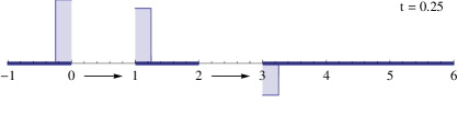
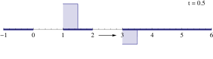
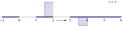
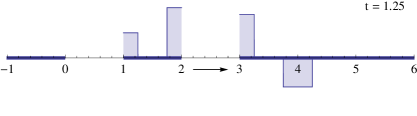
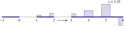
Figure 5.1. Wave-packet propagating through a double-barrier $I_{1}\cup I_{2}$ where $I_{1}=[0,1]$, $I_{2}=[2,3]$, and $\Omega=\mathbb{R}\backslash(I_{1}\cup I_{2})$. See Example 5.9.

6. Spectral representation and scattering

In this section we calculate more details regarding spectral and scattering. Since the scattering information is encoded in $L^{2}(I_{0})$, and $I_{0}$ is a finite interval, the Fourier transform of functions in $L^{2}(I_{0})$ are band-limited. As a result, by restricting one of the variables in the Shannon kernel, we get an orthonormal basis (ONB). We compute the scattering operator, and the Lax-Phillips semigroup in this ONB.

6.1. Obstacle scattering

6.1.1. Two normalizations

We continue our analysis of analysis in $L^{2}(\Omega)$ when $\Omega$ is the union of three disjoint open intervals, two infinite half-lines, and a bounded interval $I_{0}$ in the middle. As we will be working with Shannon’s kernel, it will be convenient in some computations to choose $I_{0}$ to have unit length.

1. $I_{-}=(-\infty,0)$, $I_{0}=(1,\alpha)$, and $I_{+}=(\beta,\infty)$;

2. $I_{-}=(-\infty,\tilde{\alpha})$, $I_{0}=(-\frac{1}{2},\frac{1}{2})$, and $I_{+}=(\tilde{\beta},\infty)$.

In both cases,

$$\Omega:=I_{-}\cup I_{0}\cup I_{+};$$

and let $P_{0}$ and $P_{\pm}$ be the projection operators given by multiplication:

$$P_{0}:=multi\chi_{0},\ P_{\pm}:=multi\chi_{\pm}$$

acting in the Hilbert space $L^{2}(\Omega)$.

We need the Shannon kernel for both cases.

Lemma 6.1.

Let

$$\varphi(x) = \begin{cases}1&x\in[-\frac{T}{2},\frac{T}{2}]\\ 0&\mbox{otherwise}\end{cases};$$

then $\hat{\varphi}(\lambda)=\frac{\sin(\pi\lambda T)}{\pi\lambda}$.

Proof.

This follows from a direct computation, see also [DM72].∎

Remark 6.2.

For case (1), we choose $T=1$, and the Shannon kernel is

$$Shann(x):=\frac{\sin(\pi\lambda)}{\pi\lambda}=\mbox{Sinc}(\pi\lambda).$$ (6.1)

For case (2), we choose $T=\alpha-1$ (length of the middle interval $I_{0}$), and translation $\varphi$ to the right by $(\alpha+1)/2$ (i.e., the mid-point of $I_{0}$).

$$Shann(x) :=e^{i2\pi(\frac{\alpha+1}{2})}\frac{\sin(\pi(\alpha-1)\lambda)}{\pi\lambda}$$

$$=e^{i\pi(\alpha+1)}\frac{\sin(\pi(\alpha-1)\lambda)}{\pi\lambda}$$

$$=e^{i\pi(\alpha+1)}(\alpha-1)\frac{\sin(\pi(\alpha-1)\lambda)}{\pi(\alpha-1)\lambda}$$

$$=e^{i\pi(\alpha+1)}(\alpha-1)\mbox{Sinc}(\pi(\alpha-1)\lambda).$$ (6.2)

Compare with the kernel in (6.1). Note the argument used in the proofs applies to both kernels (6.1) and (6.2).

Lemma 6.3.

The Shannon kernel on $I_{0}=(1,\alpha)$ is

$$e\left(\frac{\alpha+1}{2}\lambda\right)\frac{\sin(\pi(\alpha-1)\lambda)}{\pi\lambda}.$$

Proof.

We check that

$$\int_{1}^{\alpha}e(\lambda x)dx = \frac{1}{i2\pi\lambda}\left(e(\alpha\lambda)-e(\lambda)\right)$$

$$= \frac{1}{\pi\lambda}e\left(\frac{\alpha+1}{2}\lambda\right)\sin\left(\pi(\alpha-1)\lambda\right)$$

$$= e\left(\frac{\alpha+1}{2}\lambda\right)\frac{\sin\left(\pi(\alpha-1)\lambda\right)}{\pi\lambda}.$$

∎

6.1.2. Summary

For convenience, here is a quick summary of the comparison between the two setups:

1. If $\Omega=(-\infty,0)\cup(1,\alpha)\cup(\beta,\infty)$;
   Shannon kernel:

   $$K_{Shann}(x)=\frac{\sin(\pi\lambda T)}{\pi\lambda};$$

2. Rescaled version - $\Omega=(-\infty,\tilde{\alpha})\cup(-\frac{1}{2},\frac{1}{2})\cup(\tilde{\beta},\infty)$;
   Shannon kernel:

   $$K_{Shann}(x)=e^{i\pi(\alpha+1)}(\alpha-1)\frac{\sin(\pi(\alpha-1)\lambda)}{\pi(\alpha-1)\lambda}.$$

In both cases, the unitary group is

$$U_{B}(t)=e^{-itP_{B}},t\in\mathbb{R}$$

so that

$$\left(V_{B}U_{B}(t)f\right)(\lambda)=e(-\lambda t)\left(V_{B}f\right)(\lambda).$$

This amounts to a right-translation by $t$, i.e.,

$$f\mapsto f(\cdot-t).$$

6.2. Computation of direct integral decomposition

Fix $B(w,\theta,\phi,\psi)\in U(2)$, $0<w<1$, we have

• $P_{B}$ selfadjoint operator in $L^{2}(\Omega)$

• $\{U_{B}(t)\}_{t\in\mathbb{R}}$ acting in $L^{2}(\Omega)$; here $U_{B}(t):=e^{-itP_{B}}$.

• A unitary operator $V_{B}:L^{2}(\Omega)\rightarrow L^{2}(\mathbb{R},\sigma_{B})$, where $\sigma_{B}(d\lambda)=m^{-2}(\lambda)d\lambda$.

Let $f\in L^{2}(\Omega)$, $t,\lambda\in\mathbb{R}$, recall that

$$\left(V_{B}U_{B}(t)f\right)(\lambda)=e_{\lambda}(-t)\left(V_{B}f\right)(\lambda)$$

and

$$L^{2}(\Omega)\ni f=\int_{\mathbb{R}}^{\oplus}\left(V_{B}f\right)(\lambda)\psi_{\lambda}^{(B)}d\sigma_{B}(\lambda).$$

i.e., a direct integral decomposition.

Remark 6.4.

The transform, generalized eigenfunctions, and the measure all depend on $B$. This is indicated with the sup/sub-scripts.

Lemma 6.5.

For $f\in L^{2}(\Omega)$, we have

$$\int_{\Omega}\left|f(x)\right|^{2}dx =\int_{\mathbb{R}}\left|\left(V_{B}f\right)(\lambda)\right|^{2}d\sigma_{B}(\lambda)$$

$$\left(V_{B}f\right)(\lambda) =\int_{\Omega}\overline{\psi_{\lambda}(x)}f(x)dx$$

$$=\overline{a(\lambda)}\left(P_{-}f\right)^{\wedge}+\left(P_{0}f\right)^{\wedge}+\overline{a(\lambda)}\left(P_{+}f\right)^{\wedge}$$

where

$$\psi_{\lambda}=\psi_{\lambda}^{(B)}=a(\lambda)\chi_{-}+\chi_{0}+c(\lambda)\chi_{+}.$$

Moreover,

$$P_{-}\psi_{\lambda} = a(\lambda)e_{\lambda}\mbox{ on }I_{-}$$ (6.3)

$$P_{0}\psi_{\lambda} = e_{\lambda}\mbox{ on }I_{0}$$ (6.4)

$$P_{+}\psi_{\lambda} = c(\lambda)e_{\lambda}\mbox{ on }I_{+}.$$ (6.5)

Proof.

A direct calculation. ∎

The spectral representation is summarized in the following theorem:

Theorem 6.6.

Let $B(w,\theta,\phi,\psi)\in U(2)$ be the boundary matrix in (2.21), $0<w<1$; and let $P_{B}$ be the corresponding selfadjoint extension. The spectral representation theorem (in its fancy version) applied to $P_{B}$ as a selfadjoint operator in $L^{2}(\Omega)$ has multiplicity-one, and its direct integral measure is $d\sigma_{B}(\lambda):=m^{-2}(\lambda)d\lambda$ on the whole Hilbert space $L^{2}(\Omega)$.

6.3. Shannon kernel and scattering

Suppose we are in case (1), i.e., the middle interval is $I_{0}=[-\frac{1}{2},\frac{1}{2}]$. The Shannon kernel is

$$K(\lambda,\xi)=\frac{\sin(\pi(\lambda-\xi))}{\pi(\lambda-\xi)},\;\lambda,\xi\in\mathbb{R};$$ (6.6)

See [DM72] for its properties.

Recall that the Shannon is the kernel of the projection operator onto the the space of band-limited functions:

$$BL:=\{\hat{f}(\cdot);\chi_{I_{0}}f=f\}\subset L^{2}(\mathbb{R},d\lambda).$$

Note the identifications:

$$f\in L^{2}(I_{0})\Longleftrightarrow\{f\in L^{2}(\Omega);\chi_{I_{0}}f=f\}$$

and

$$L^{2}(I_{0})\simeq P_{0}L^{2}(\Omega).$$

So,

$$f\in L^{2}(I_{0})\Longleftrightarrow\hat{f}\in BL.$$

Lemma 6.7 (Shannon Interpolation).

If $f\in L^{2}(I_{0})=P_{0}L^{2}(\Omega)$, then

$$\hat{f}(\lambda)=\sum_{n\in\mathbb{Z}}\hat{f}(n)\frac{\sin\pi(\lambda-n)}{\pi(\lambda-n)}$$

and $\left\{\frac{\sin\pi(\lambda-n)}{\pi(\lambda-n)}\right\}_{n\in\mathbb{Z}}$ is an ONB in $BL$ (band-limited functions, frequency band = $[-\frac{1}{2},\frac{1}{2}]$).

Proof.

A calculation, see e.g., [DM72]. ∎

6.4. Computation of the scattering semigroup

In our model $\Omega$ has two unbounded components, and one bounded $I_{0}$ in the middle. (By rescaling we may arrange that $I_{0}$ has unit length.) In the language of Lax-Phillips [LP68], $I_{0}$ then represents "obstacle" for the unitary one-parameter group $U_{B}(t)$ transforming the global states. As predicted by [LP68], we show below that the cut-down of $U_{B}(t)$ will then be a contraction semigroup (now in $L^{2}(I_{0})$). We are further able to compute this semigroup and show how it depends on the unitary matrix $B$ classifying our selfadjoint extension operators. Moreover we show that the semigroup carries detailed scattering information; and it is also of relevance to model theory; see [JM80].

6.4.1. Key lemmas

Recall some key steps that will be used below.

Lemma 6.8.

If $f\in L^{2}(I_{0})$, then

$$\left(V_{B}f\right)(\lambda)=\hat{f}(\lambda).$$ (6.7)

Proof.

In fact,

$$\left(V_{B}f\right)(\lambda) =\left\langle\psi_{\lambda}^{(B)},f\right\rangle_{\Omega}=\left\langle\psi_{\lambda}^{(B)},P_{0}f\right\rangle_{\Omega}=\left\langle P_{0}\psi_{\lambda}^{(B)},f\right\rangle_{\Omega}$$

$$=\left\langle e_{\lambda},f\right\rangle_{\Omega}=\int_{I_{0}}\overline{e_{\lambda}(x)}f(x)dx=\hat{f}(\lambda).$$

See (6.4).∎

Lemma 6.9.

If $f\in L^{2}(I_{0})$ then

$$f=\int_{\mathbb{R}}\hat{f}(\lambda)e_{\lambda}d\sigma_{B}(\lambda).$$

In particular, for all $x\in I_{0}$,

$$f(x)=\left(m^{-2}\hat{f}\right)^{\vee}(x)=\sum_{n\in\mathbb{Z}}a_{n}f(x+n)$$

where

$$m^{-2}(\lambda)=\sum_{n\in\mathbb{Z}}a_{n}e_{n}(\lambda)$$

is the Fourier series.

Proof.

By (6.7), we get

$$f=\int_{\mathbb{R}}\hat{f}(\lambda)\psi_{\lambda}^{(B)}d\sigma_{B}(\lambda).$$

Apply $P_{0}$ on both sides, we get

$$f=P_{0}f =\int_{\mathbb{R}}\hat{f}(\lambda)P_{0}\psi_{\lambda}^{(B)}d\sigma_{B}(\lambda)$$

$$=\int_{\mathbb{R}}\hat{f}(\lambda)e_{\lambda}d\sigma_{B}(\lambda)$$

by (6.4).∎

Corollary 6.10.

$\hat{f}\mapsto\widehat{Z_{B}(t)f}$ is expressed in terms of $K_{Shann}$ as

$$\widehat{Z_{B}(t)f}(\lambda)=\int_{\mathbb{R}}\frac{\sin\pi(\lambda-\xi)}{\pi(\lambda-\xi)}e_{\xi}(-t)\hat{f}(\xi)d\sigma_{B}(\lambda).$$ (6.8)

Moreover,

$$\sum_{n\in\mathbb{Z}}\left|\widehat{Z_{B}(t)f}(n)\right|^{2}\leq\frac{4}{w^{2}}\left\|f\right\|_{\Omega}^{2}.$$

Proof.

Here we use the middle interval $I_{0}=[-\frac{1}{2},\frac{1}{2}]$, so the kernel is given in (6.6). By Lemma 6.9, we have

$$\left(Z_{B}(t)f\right)(x) = \chi_{0}\left(e(-\lambda t)m^{-2}(\lambda)\hat{f}(\lambda)\right)^{\vee}$$ (6.9)

$$= \left(\widehat{\chi_{0}}*\left(e_{\lambda}(-t)m^{-2}\hat{f}\right)\right)^{\vee}$$

$$= \int_{\mathbb{R}}\frac{\sin\pi(\lambda-\xi)}{\pi(\lambda-\xi)}e_{\xi}(-t)\hat{f}(\xi)d\sigma_{B}(\xi).$$

Using the interpolation formula, the RHS above is

$$RHS =\sum_{n\in\mathbb{Z}}\widehat{Z_{B}(t)f}(n)\frac{\sin\pi(\lambda-n)}{\pi(\lambda-n)}$$

$$=\sum_{n\in\mathbb{Z}}\int_{\mathbb{R}}\frac{\sin\pi(\lambda-\xi)}{\pi(\lambda-\xi)}e_{\xi}(-t)\hat{f}(\xi)d\sigma_{B}(\xi)\times\frac{\sin\pi(\lambda-n)}{\pi(\lambda-n)};$$

and

$$\sum_{n\in\mathbb{Z}}\left|\widehat{Z_{B}(t)f}(n)\right|^{2} =\int_{\mathbb{R}}\left|\widehat{Z_{B}(t)f}(\lambda)\right|^{2}d\lambda\mbox{ (Parseval + Shannon ONB in BL)}$$

$$=\int_{\mathbb{R}}\left|m(\lambda)\right|^{2}\left|\widehat{Z_{B}(t)f}(\lambda)\right|^{2}d\sigma_{B}(\lambda)$$

$$\leq\frac{4}{w^{2}}\int\left|\widehat{Z_{B}(t)f}(\lambda)\right|^{2}d\sigma_{B}(\lambda)$$

$$=\frac{4}{w^{2}}\left\|Z_{B}(t)f\right\|_{\Omega}^{2}\leq\frac{4}{w^{2}}\left\|f\right\|_{\Omega}^{2}.$$

Note the last two steps follows from Prop 7.1. ∎

6.4.2. Semigroups

Below we derive explicit formulas for the Lax-Phillips semigroup $Z_{B}(t)$ making use of Shannon’s kernel, as well as the Shannon interpolation formula (see e.g., [DM72].) This material leads up to Theorem 6.18, giving a formula for the analytic resolvent operator $R_{B}(\cdot)$, analytic in the complex right-half plane, and computed from the infinitesimal generator of $Z_{B}(t)$.

Theorem 6.11.

$Z_{B}(t):=P_{0}U_{B}(t)P_{0}:L^{2}(I_{0})\rightarrow L^{2}(I_{0})$, $t\geq 0$, is a contraction semigroup, i.e.

1. For all $s,t\geq 0$,

   $$Z_{B}(t)Z_{B}(s)=Z_{B}(t+s);$$ (6.10)

2. $Z_{B}(0)=P_{0}$, acting as the identity operator in $L^{2}(I_{0})$.

Proof.

For all $f\in L^{2}(I_{0})$, and $t>0$,

$$\left\|Z_{B}(t)f\right\|_{I_{0}} =\left\|P_{0}U_{B}(t)P_{0}f\right\|_{\Omega}$$

$$\leq\left\|U_{B}(t)P_{0}f\right\|_{\Omega}=\left\|P_{0}f\right\|_{\Omega}=\left\|f\right\|_{I_{0}}$$

since $\left\|P_{0}\right\|_{L^{2}(\Omega)\rightarrow L^{2}(\Omega)}\leq 1$, i.e., the projection $P_{0}$ is contractive. This proves that $\left\|Z_{B}(t)\right\|_{I_{0}}\leq 1$.

Let $s,t\geq 0$, then

$$Z_{B}(s)Z_{B}(t) = P_{0}U_{B}(s)P_{0}U_{B}(t)P_{0}$$ (6.11)

$$= P_{0}U_{B}(s)\left(P_{(\beta,\infty)}^{\perp}P_{(-\infty,0)}^{\perp}\right)U_{B}(t)P_{0}$$

$$= \left(P_{0}U_{B}(s)P_{(\beta,\infty)}^{\perp}\right)\left(P_{(-\infty,0)}^{\perp}U_{B}(t)P_{0}\right)$$

$$= \left(P_{(\beta,\infty)}^{\perp}U_{B}(-s)P_{0}\right)^{*}\left(P_{(-\infty,0)}^{\perp}U_{B}(t)P_{0}\right).$$

Since for $s\geq 0$, we have $U_{B}(s)L^{2}(I_{+})\subset L^{2}(I_{+})$, and it follows that

$$P_{(\beta,\infty)}^{\perp}U_{B}(-s)P_{0}=U_{B}(-s)P_{0}.$$

Similarly, $t\geq 0$ implies that

$$P_{(-\infty,0)}^{\perp}U_{B}(t)P_{0}=U_{B}(t)P_{0}.$$

Therefore, (6.11) reads

$$Z_{B}(s)Z_{B}(t) = \left(U_{B}(-s)P_{0}\right)^{*}\left(U_{B}(t)P_{0}\right)$$

$$= \left(P_{0}U_{B}(s)\right)\left(U_{B}(t)P_{0}\right)$$

$$= P_{0}U_{B}(s+t)P_{0}.$$

This shows that $Z_{B}(t)$ satisfies the semigroup law in (6.10).

Clearly, $Z_{B}(0)=P_{0}$; and this completes the proof of the theorem. ∎

The semigroup law (6.10) can be checked directly using the Shannon kernels.

Here we are still in case (2), where the middle interval is $I_{0}=[-\frac{1}{2},\frac{1}{2}]$. But the same argument applies to $I_{0}=[1,\alpha]$ as well. Recall the infinitesimal generator $G_{B}$ of $Z_{B}(t)$ is

$$G_{B}f:=\frac{1}{2\pi i}\lim_{t\rightarrow 0_{+}}\frac{1}{t}\left(Z_{B}(t)f-f\right)$$

with $dom(G_{B})=\{f\in L^{2}(I_{0}):\mbox{ the above limit exits}\}$. That is,

$$\mathscr{D}(G_{B})=\{f\in L^{2}(I_{0});\int_{\mathbb{R}}\left|\hat{f}(\lambda)\right|^{2}\lambda^{2}d\lambda<\infty\}.$$

For motivations, see [LP68].

Direct proof of Theorem 6.11.

Let $s,t\geq 0$, $f\in L^{2}(I_{0})$, recall that

$$\widehat{Z_{B}(t)f}(\lambda)=\int_{\mathbb{R}}\frac{\sin\pi(\xi-\lambda)}{\pi(\xi-\lambda)}e_{\xi}(-t)\hat{f}(\xi)d\sigma_{B}(\xi);$$

so that

$$\left(Z_{B}(s)Z_{B}(t)f\right)^{\wedge}(\lambda)$$

$$= \int_{\mathbb{R}}\frac{\sin\pi(\xi-\lambda)}{\pi(\xi-\lambda)}e_{\xi}(-s)\widehat{Z_{B}(t)f}(\xi)d\sigma_{B}(\xi)$$

$$= \int_{\mathbb{R}}\frac{\sin\pi(\xi-\lambda)}{\pi(\xi-\lambda)}e_{\xi}(-s)\left(\int_{\mathbb{R}}\frac{\sin\pi(\eta-\xi)}{\pi(\eta-\xi)}e_{\xi}(-t)\hat{f}(\eta)d\sigma_{B}(\eta)\right)d\sigma_{B}(\xi)$$

$$= \iint_{\mathbb{R}}\frac{\sin\pi(\xi-\lambda)}{\pi(\xi-\lambda)}\frac{\sin\pi(\eta-\xi)}{\pi(\eta-\xi)}e_{\xi}(-s)e_{\xi}(-t)\hat{f}(\eta)d\sigma_{B}(\eta)d\sigma_{B}(\xi)$$

$$= \int_{\mathbb{R}}\left(\int_{\mathbb{R}}\frac{\sin\pi(\xi-\lambda)}{\pi(\xi-\lambda)}\frac{\sin\pi(\eta-\xi)}{\pi(\eta-\xi)}e_{\xi}(-t)d\sigma_{B}(\xi)\right)e_{\xi}(-s)\hat{f}(\eta)d\sigma_{B}(\eta)$$

It suffices to show that

$$\int_{\mathbb{R}}\frac{\sin\pi(\xi-\lambda)}{\pi(\xi-\lambda)}\frac{\sin\pi(\eta-\xi)}{\pi(\eta-\xi)}e_{\xi}(-t)d\sigma_{B}(\xi)=\frac{\sin\pi(\eta-\lambda)}{\pi(\eta-\lambda)}e_{\eta}(-t).$$ (6.12)

Note that

$$\frac{\sin\pi(\cdot-\lambda)}{\pi(\cdot-\lambda)},\;\frac{\sin\pi(\eta-\cdot)}{\pi(\eta-\cdot)}\in BL;$$

hence the measure $d\sigma_{B}(\xi)$ on the LHS in (6.12) can be replaced by $d\xi$, i.e., the usual Lebesgue measure; and the result follows from this. ∎

6.4.3. Summary of results on $Z_{B}(t)$

Recall the two setups:

$$\Omega=(-\infty,0)\cup(1,\alpha)\cup(\beta,\infty)$$

and

$$\tilde{\Omega}=(-\infty,\tilde{\alpha})\cup(-\frac{1}{2},\frac{1}{2})\cup(\tilde{\beta},\infty).$$

In both cases

$$\left(Z_{B}(t)f\right)^{\wedge}(\lambda)=\int_{\mathbb{R}}\hat{f}(\xi)K_{Shann}(\xi,\lambda)e_{\xi}(-t)d\sigma_{B}(\xi)$$

for all $\lambda,t\in\mathbb{R}$, and all $f\in L^{2}(I_{0})$. Note that

$$f\in L^{2}(I_{0})\Longleftrightarrow\hat{f}\in BL=\widehat{L^{2}(I_{0})}.$$

$\widehat{Z_{B}(t)}$ can be seen as defined by

$$BL\ni\hat{f}\mapsto\widehat{Z_{B}(t)f}\in BL;$$

then the transform $\widehat{Z_{B}(t)}$ is an integral operator

$$\hat{f}\mapsto\int_{\mathbb{R}}K_{Shann}(\xi,\lambda)e_{\xi}(-t)\hat{f}(\xi)d\sigma_{B}(\xi).$$

See eq. (6.8).

Remark 6.12.

A few observations:

1. The Fourier basis $\{e_{n}\}_{n\in\mathbb{Z}}$ is an ONB in $L^{2}(I_{0})\subset L^{2}(\Omega)$, but $\{e_{n}\}_{n\in\mathbb{Z}}$ do not belong to $\mathscr{D}(P_{B})$, $0<w<1$. In deed, the generalized eigenfunction of $P_{B}$, as a selfadjoint operator in $L^{2}(\Omega)$, are

   $$\psi_{\lambda}^{(B)}=a^{(B)}(\lambda)e_{\lambda}\chi_{I_{-}}+e_{\lambda}\chi_{I_{0}}+c_{\lambda}^{(B)}(\lambda)e_{\lambda}\chi_{I_{+}};$$

   and $a^{(B)}(\lambda)$, $c^{(B)}(\lambda)$ are NOT constants, see Lemma 3.17 for an estimate, where

   $$\left|a^{(B)}(\lambda)\right|=\left|c^{(B)}(\lambda)\right|\in[-\frac{w}{2},\frac{w}{2}].$$

   Note $P_{0}\mathscr{D}(P_{B})\nsubseteq\mathscr{D}(P_{B})$ with $0<w<1$, so

   $$P_{0}\psi_{\lambda}^{(B)}=e_{\lambda}\chi_{I_{0}}\in\mathscr{D}(P_{B})$$

   and so when $\lambda=n$,

   $$e_{n}\chi_{I_{0}}\notin\mathscr{D}(P_{B}).$$

2. $Z_{B}(t)$ acts in $L^{2}(I_{0})$, and it is zero on $L^{2}(I_{-})\oplus L^{2}(I_{+})$.

Remark 6.13.

We have

$$\left(Z_{B}(t)\chi_{I_{0}}e_{n}\right)(x)=\chi_{0}(x)\int_{\mathbb{R}}\frac{\sin\pi(\lambda-n)}{\pi(\lambda-n)}e_{\lambda}(x-t)d\sigma_{B}(\lambda).$$ (6.13)

Proof.

Recall that

$$\left(Z_{B}(t)f\right)(x) = \chi_{0}\left(e(-\lambda t)m^{-2}\hat{f}\right)^{\vee}$$

$$= \chi_{0}(x)\int e(-\lambda t)e(\lambda x)\hat{f}(\lambda)d\sigma_{B}(\lambda)$$

$$= \chi_{0}(x)\int e_{\lambda}(x-t)\hat{f}(\lambda)d\sigma_{B}(\lambda).$$

Now, apply this to $f(x):=\chi_{I_{0}}e_{n}$. Note that $\hat{f}$ is the Shannon kernel.∎

Corollary 6.14 (application of (6.13) ).

$$\left\|Z_{B}(t)e_{n}\chi_{0}\right\|^{2}=\left|I_{0}\cap(I_{0}+t)\right|=\max(1-t,0),\;t\in\mathbb{R}_{+}.$$

Remark 6.15.

For all $f\in L^{2}(I_{0})$, we define

$$\left(W_{0}f\right)(x):=\int\hat{f}(\lambda)e_{\lambda}(x)d\sigma_{B}(\lambda)=\left(m^{-2}\hat{f}\right)^{\vee}(x).$$

From previous discussion, we see that

$$\left(Z_{B}(t)f\right)(x)=P_{0}\left(W_{0}f\right)(x-t).$$

Figure 6.1 below illustrates the semigroup law of $Z_{B}(t)$, $t\geq 0$.

$f$	$f$
$W_{0}f$	$Z_{B}(t)f=\chi_{0}(W_{0}f)(\cdot-t)$
$(W_{0}f)(\cdot-t)$	$W_{0}Z_{B}(t)f$
$(W_{0}f)(\cdot-s-t)$	$(W_{0}Z_{B}(t)f)(\cdot-s)$
$Z_{B}(s+t)f$	$Z_{B}(s)Z_{B}(t)f$

Figure 6.1. $Z_{B}(s+t)f$

Remark 6.16.

Let $I_{0}=(1,\alpha)$. We proved in Theorem 6.11 that, in the general case, the semigroup

$$Z_{B}(t)=P_{0}U_{B}(t)P_{0}:L^{2}(I_{0})\rightarrow L^{2}(I_{0}),$$ (6.14)

defined for $t\in\mathbb{R}_{+}$, can be computed from the simpler spatial semigroup $Z_{sp}(t):L^{2}(I_{0})\rightarrow L^{2}(I_{0})$ given by

$$\left(Z_{sp}(t)f\right)(x)=\chi_{I_{0}}(x)f(x-t),\;f\in L^{2}(I_{0}),t>0.$$ (6.15)

Hence, the generator, and the resolvent operator for $Z_{B}(t)$ in (6.15) may be computed from (6.15). One checks that the domain of the infinitesimal generator $G_{sp}$ in (6.15) is

$$\mathscr{D}(G_{sp})=\{f\in L^{2}(I_{0});f^{\prime}\in L^{2}(I_{0}),\mbox{ and }f(1)=0\}.$$

Recall $x=1$ is the left endpoint in $I_{0}$. If $\lambda\in\mathbb{C}$, and $\Re\lambda>0$ then the resolvent operator $R_{sp}(\lambda)=(\lambda I-G_{sp})^{-1}$ for (6.15) is the following Volterra integral operator (see [Mat10])

$$\left(R_{sp}(\lambda)f\right)(x)=\int_{1}^{x}e^{-\lambda(x-y)}f(y)dy,$$ (6.16)

defined for all $f\in L^{2}(I_{0})$, and $x\in I_{0}$ ($=(1,\alpha)$.) The Volterra property of (6.16) reflects causality for the scattering we computed in section 6.1, see also [LP68].

6.5. The resolvent family of $Z_{B}(t)$

Let $\Omega=I_{-}\cup I_{0}\cup I_{+}=(-\infty,0)\cup(1,\alpha)\cup(\beta,\infty)$ be as above, i.e., $1<\alpha<\beta<\infty$ are fixed, and we set $I_{0}=(1,\alpha)$. Fix $B\in U(2)$ such that $w>0$, and set

$$Z_{B}(t)=P_{0}U_{B}(t)P_{0},t\in\mathbb{R}_{+}.$$ (6.17)

Here $P_{0}$ denotes the projection of $L^{2}(\Omega)$ onto the subspace $L^{2}(I_{0})\subset L^{2}(\Omega)$, i.e.,

$$P_{0}f=\chi_{I_{0}}f,$$ (6.18)

for all $f\in L^{2}(\Omega)$.

In this section, we shall compare the two $C_{0}$-semigroups $Z_{B}(t)$ and $Z_{sp}(t)$ from sect 6.4 and Remark 6.16. Recall, $Z_{sp}(t)$ is the spatial semigroup in $L^{2}(I_{0})$ given, for $t\in\mathbb{R}_{+}$, by right-translation by $t$, followed by truncation; i.e., $Z_{sp}(t)f=0$ if $t>\alpha-1=\mbox{length}(I_{0})$, see (6.15).

Both $\left(Z_{B}(t)\right)$ and $\left(Z_{sp}(t)\right)$ are $C_{0}$-semigroup of contraction operators in $L^{2}(I_{0})$.

Lemma 6.17 ([LP68]).

Let $\mathscr{H}_{0}$ be a Hilbert space, and let $\{Z(t)\}_{t\in\mathbb{R}_{+}}$ be a contraction semigroup in $\mathscr{H}_{0}$. Then there is a dense subspace $\mathscr{D}(G)$ in $\mathscr{H}_{0}$ such that, for $f\in\mathscr{D}(G)$, the limit

$$\lim_{t\rightarrow 0_{+}}\frac{1}{t}\left(Z(t)f-f\right)=Gf$$ (6.19)

exists. The operator $G$ is called the infinitesimal generator. For $\lambda\in\mathbb{C}$, $\Re\lambda>0$, the resolvent operator

$$R(\lambda)=(\lambda I-G)^{-1}:\mathscr{H}_{0}\rightarrow\mathscr{H}_{0}$$ (6.20)

is an analytic family of bounded operators. We have

$$\left\|R_{G}(\lambda)\right\|_{\mathscr{H}_{0}\rightarrow\mathscr{H}_{0}}\leq\frac{1}{\Re\lambda}$$ (6.21)

for $\Re\lambda>0$; and moreover the following two limits hold in the strong operator-topology:

$$R_{G}(\lambda)=\int_{0}^{\infty}e^{-t\lambda}Z(t)dt,\mbox{ and }$$ (6.22)

$$\lim_{n\rightarrow\infty}\left(\frac{n}{t}R_{G}\left(\frac{n}{t}\right)\right)^{n}=Z(t),\>t\in\mathbb{R}_{+}.$$ (6.23)

Proof.

See [LP68]. ∎

From (6.23), we see in particular that a given semigroup is determined uniquely by its infinitesimal generator.

Theorem 6.18.

Now fix $B\in U(2)$ such that $w_{B}>0$, and denote the infinitesimal generator of $Z_{B}(t)$ by $G_{B}$ i.e., for $f\in\mathscr{D}(G_{B})$, we have

$$\lim_{t\rightarrow 0_{+}}\frac{1}{t}\left(Z_{B}(t)f-f\right)=G_{B}f,$$

see (6.19). For $\lambda\in\mathbb{C}$, $\Re\lambda>0$, set

$$R_{B}(\lambda):=\left(\lambda I-G_{B}\right)^{-1}.$$ (6.24)

Finally we introduce the function $m_{B}(\cdot)$ from Lemma 3.17, i.e.,

$$\mathbb{R}\ni\xi\mapsto m_{B}(\xi)\in\mathbb{R}_{+}.$$ (6.25)

Then for all $\lambda\in\mathbb{C}$, $\Re\lambda>0$, we have

$$R_{B}(\lambda)=R_{sp}\left(\lambda m_{B}(0)^{2}\right):L^{2}(I_{0})\rightarrow L^{2}(I_{0}),$$ (6.26)

where $R_{sp}(\cdot)$ is the resolvent family from (6.16) in Remark 6.16.

Proof.

We introduce the following notation, based on Corollary 5.6. Let $B\in U(2)$ be as above, i.e., $B=B(w,\phi,\psi,\theta)$, and assume $w>0$. For $f\in L^{2}(I_{0})$, set

$$\left(E_{B}f\right)(x) :=\left(m_{B}^{-2}\hat{f}\right)^{\vee}(x)$$ (6.27)

$$=\sum_{k\in\mathbb{Z}}a_{k}f(x+k(\alpha-1))$$

where $(a_{k})_{k\in\mathbb{Z}}$ is the set of Fourier coefficients of $m_{B}^{-2}$, i.e.,

$$a_{k}=(1-w^{2})^{\frac{\left|k\right|}{2}}e(-k\psi),\>k\in\mathbb{Z},$$ (6.28)

and

$$m^{-2}(\xi)=\sum_{k\in\mathbb{Z}}a_{k}e_{k}((\alpha-1)\xi),\>\xi\in\mathbb{R}.$$ (6.29)

For the semigroup $\left(Z_{B}(t)\right)_{t\in\mathbb{R}_{+}}$ we proved in section 5 that

$$\left(Z_{B}(t)f\right)(x)=\chi_{I_{0}}(x)\left(E_{B}f\right)(x-t),\ x\in I_{0},t>0.$$

Using (6.29) we get

$$1=\sum_{k\in\mathbb{Z}}m_{B}(0)^{2}a_{k}.$$ (6.30)

Using the argument for Remark 6.16, and (6.30), the desired formula (6.26) follows. ∎

7. Intervals versus Points

There are good reasons to consider the cases when the scattering by intervals degenerate to points. Obstacle scattering, both for the acoustic wave equations and for quantum theory, behaves differently in the degenerate cases. In quantum mechanics one studies what happens at quantum scale; and wave-particle duality of matter is realized experimentally, for example in quantum-tunneling: the phenomenon where a particle/wave-function tunnels through a barrier (which could not have been surmounted by a classical particle.) It is often explained with use of the Heisenberg uncertainty principle. So quantum tunneling is one of the defining features of quantum mechanics. Quantum differs from classical mechanics in this way. Classical mechanics predicts that particles that do not have enough energy to classically surmount a barrier will not be able to reach the other side. By contrast, in quantum mechanics, particles behave as waves and can, with positive probability, tunnel through the barrier.

7.1. Deleting one point

Let $U_{t}:=e^{itP_{\theta}}$. Let $\Omega:=\mathbb{R}\setminus\{0\}.$ Let $\chi_{-}:=\chi_{(-\infty,0)}$ and $\chi_{+}:=\chi_{(0,\infty)}.$ The generalized eigenfunctions are

$$\psi_{\xi}(x):=e(x\xi)\left(e(\theta)\chi_{-}(x)+\chi_{+}(x)\right),\xi\in\mathbb{R}.$$

Define $V:L^{2}(\mathbb{R})\to L^{2}(\Omega),$ (of course $L^{2}(\Omega)=L^{2}(\mathbb{R})$ but the distinction is important below) by

$$Vf(x) :=\left(e(\theta)\chi_{-}(x)+\chi_{+}(x)\right)f(x)$$

$$=\int_{\mathbb{R}}\widehat{f}(\xi)e(x\xi)\left(e(\theta)\chi_{-}(x)+\chi_{+}(x)\right)d\xi$$

$$=\int_{\mathbb{R}}\widehat{f}(\xi)\psi_{\xi}(x)d\xi$$

where we used $f(x)=\int_{\mathbb{R}}\widehat{f}(\xi)e(x\xi)d\xi.$ Since $\psi_{\xi}$ is a generalized eigenfunction

$$U_{t}Vf(x) =\int_{\mathbb{R}}\widehat{f}(\xi)e(t\xi)e(\xi x)\left(e(\theta)\chi_{-}(x)+\chi_{+}(x)\right)d\xi.$$

Consequently, $V^{*}g(x)=\left(e(-\theta)\chi_{-}(x)+\chi_{+}(x)\right)g(x)$ and

$$\left(e(-\theta)\chi_{-}(x)+\chi_{+}(x)\right)\left(e(\theta)\chi_{-}(x)+\chi_{+}(x)\right)=1$$

implies

$$V^{*}U_{t}Vf(x) =\int_{\mathbb{R}}\widehat{f}(\xi)e(t\xi)e(x\xi)d\xi=f(x+t)$$

for all $f\in L^{2}(\mathbb{R})$ and all $x,t\in\mathbb{R}.$

7.2. Deleting an interval

Let $\Omega:=\mathbb{R}\setminus(0,\alpha).$ Let $\chi_{-}:=\chi_{(-\infty,0)}$ and $\chi_{+}:=\chi_{(\alpha,\infty)}.$ The generalized eigenfunctions are

$$\psi_{\xi}(x):=e(x\xi)\left(e(\theta)\chi_{-}(x)+e(-\xi\alpha)\chi_{+}(x)\right),\xi\in\mathbb{R}.$$

Define $V:L^{2}(\mathbb{R})\to L^{2}(\Omega),$ (of course $L^{2}(\Omega)\varsubsetneqq L^{2}(\mathbb{R})$) by

$$Vf(x) :=e(\theta)f(x)\chi_{-}(x)+f(x-\alpha)\chi_{+}(x)$$

$$=\int_{\mathbb{R}}\widehat{f}(\xi)e(x\xi)\left(e(\theta)\chi_{-}(x)+e(-\xi\alpha)\chi_{+}(x)\right)d\xi$$

$$=\int_{\mathbb{R}}\widehat{f}(\xi)\psi_{\xi}(x)d\xi$$

where we used $f(x)=\int_{\mathbb{R}}\widehat{f}(\xi)e(x\xi)d\xi$ so that $f(x-\alpha)=\int_{\mathbb{R}}\widehat{f}(\xi)e(-\xi\alpha)e(x\xi)d\xi.$ Since $\psi_{\xi}$ is a generalized eigenfunction

$$U_{t}Vf(x) =\int_{\mathbb{R}}\widehat{f}(\xi)e(t\xi)e(\xi x)\left(e(\theta)\chi_{-}(x)+e(\xi\alpha)\chi_{+}(x)\right)d\xi.$$

Consequently, $V^{*}g(x)=e(-\theta)g(x)\chi_{-}(x)+g(x+\alpha)\chi_{(0,\infty)}(x)$ and $\chi_{+}(x+\alpha)=\chi_{(0,\infty)}(x)$ implies

$$V^{*}U_{t}Vf(x) =V^{*}\int_{\mathbb{R}}\widehat{f}(\xi)e(t\xi)\left(e(\theta)e(\xi x)\chi_{-}(x)+e(-\xi\alpha)e(\xi x)\chi_{+}(x)\right)d\xi$$

$$=\int_{\mathbb{R}}\widehat{f}(\xi)e(t\xi)\left(e(\xi x)\chi_{-}(x)+e(-\xi\alpha)e(\xi(x+\alpha))\chi_{(0,\infty)}(x)\right)d\xi$$

$$=\int_{\mathbb{R}}\widehat{f}(\xi)e(t\xi)e(x\xi)d\xi=f(x+t)$$

for all $f\in L^{2}(\mathbb{R})$ and all $x,t\in\mathbb{R}.$

7.3. Deleting two points

Let $\Omega=(-\infty,0)\cup(0,\alpha)\cup(\alpha,\infty).$ Let $\chi_{-}:=\chi_{(-\infty,0)},$ $\chi_{0}:=\chi_{(0,\alpha)},$$\chi_{+}:=\chi_{(\alpha,\infty)}.$

Suppose $0<w<1$ and the remaining parameters are zero. The generalized eigenfunctions are

$$\psi_{\xi}(x):=e(x\xi)\left(a(\xi)\chi_{-}(x)+\chi_{0}(x)+c(\xi)\chi_{+}(x)\right),\xi\in\mathbb{R}.$$

Define $V:L^{2}(\mathbb{R})\to L^{2}(\Omega),$ (of course $L^{2}(\Omega)=L^{2}(\mathbb{R})$) by

$$Vf(x):=\int_{\mathbb{R}}\widehat{f}(\xi)\psi_{\xi}(x)d\xi.$$

Since $\psi_{\xi}$ is a generalized eigenfunction

$$U_{t}Vf(x) =\int_{\mathbb{R}}\widehat{f}(\xi)e(t\xi)\psi_{\xi}(x)d\xi.$$

Using $a(\xi)=\overline{c(\xi)}=\frac{1}{w}\left(1-\sqrt{1-w^{2}}e(\xi\alpha)\right),$ we get

$$Vf(x) =\int_{\mathbb{R}}\widehat{f}(\xi)e(x\xi)\left(a(\xi)\chi_{-}(x)+\chi_{0}(x)+c(\xi)\chi_{+}(x)\right)d\xi$$

$$=\left(\frac{1}{w}f(x)-\frac{\sqrt{1-w^{2}}}{w}f(x+\alpha)\right)\chi_{-}(x)$$

$$\quad+f(x)\chi_{0}(x)+\left(\frac{1}{w}f(x)-\frac{\sqrt{1-w^{2}}}{w}f(x-\alpha)\right)\chi_{+}(x).$$

Hence, for $g\in L^{2}(\Omega)$ we have

$$V^{*}g(x) =\left(\frac{1}{w}g(x)-\frac{\sqrt{1-w^{2}}}{w}g(x-\alpha)\right)\chi_{-}(x)$$

$$\quad+g(x)\chi_{0}(x)+\left(\frac{1}{w}g(x)-\frac{\sqrt{1-w^{2}}}{w}g(x+\alpha)\right)\chi_{+}(x).$$

Trying $g=\psi_{\xi}$ we get

$$V^{*}\psi_{\xi}(x) =\left(\frac{1}{w}\psi_{\xi}(x)-\frac{\sqrt{1-w^{2}}}{w}\psi_{\xi}(x-\alpha)\right)\chi_{-}(x)$$

$$\quad+\psi_{\xi}(x)\chi_{0}(x)+\left(\frac{1}{w}\psi_{\xi}(x)-\frac{\sqrt{1-w^{2}}}{w}\psi_{\xi}(x+\alpha)\right)\chi_{+}(x)$$

$$=e(x\xi)a(\xi)\left(\frac{1}{w}-\frac{\sqrt{1-w^{2}}}{w}e(-\alpha\xi)\right)\chi_{-}(x)$$

$$\quad+e(x\xi)\chi_{0}+e(x\xi)c(\xi)\left(\frac{1}{w}-\frac{\sqrt{1-w^{2}}}{w}e(\alpha\xi)\right)\chi_{+}(x)$$

$$=e(x\xi)\left(\left|a(\xi)\right|^{2}\chi_{-}+\chi_{0}+\left|a(\xi)\right|^{2}\chi_{+}\right)(x).$$

Consequently,

$$V^{*}U_{t}Vf(x) =V^{*}\int_{\mathbb{R}}\widehat{f}(\xi)e(t\xi)\psi_{\xi}(x)d\xi$$

$$=\int_{\mathbb{R}}\widehat{f}(\xi)e(t\xi)e(x\xi)\left(\left|a(\xi)\right|^{2}\chi_{-}+\chi_{0}+\left|c(\xi)\right|^{2}\chi_{+}\right)(x)d\xi.$$

Where

$$\left|a(\xi)\right|^{2}=\left|c(\xi)\right|^{2}=\frac{2-w^{2}}{w^{2}}-\frac{2\sqrt{1-w^{2}}}{w^{2}}\cos(\alpha\xi).$$

Proposition 7.1.

If $\Omega$ is the complement of two points, then the associated Fourier multiplier $\left|a\left(\xi\right)\right|$ is positive, bounded, and bounded away from zero. Specifically,

$$\frac{w}{2}\leq\left|a\left(\xi\right)\right|\leq\frac{2}{w}.$$

Proof.

Note that

$$\left|a(\xi)\right| =\left|\frac{1}{w}-\frac{\sqrt{1-w^{2}}}{w}e(\alpha\xi)\right|\geq\frac{1}{w}-\frac{\sqrt{1-w^{2}}}{w}$$

$$=\frac{1}{w}\left(1-\sqrt{1-w^{2}}\right)\geq\frac{1}{w}\left(1-\left(1-\frac{1}{2}w^{2}\right)\right)=\frac{w}{2}.$$

On the other hand,

$$\left|a(\xi)\right|=\left|\frac{1}{w}-\frac{\sqrt{1-w^{2}}}{w}e(\alpha\xi)\right|\leq\frac{1}{w}+\frac{\sqrt{1-w^{2}}}{w}\leq\frac{2}{w}.$$

∎

8. Vanishing Cross-terms

We include a direct computation to show the cross-terms in (3.50) all vanish.

Let $\Omega=(-\infty,0)\cup(1,\alpha)\cup(\beta,\infty)$. For all $f\in L^{2}(\Omega)$, write

$$f=f_{-}+f_{0}+f_{+}$$

where $f_{-}=\chi_{-}f$, $f_{0}=\chi_{0}f$, and $f_{+}=\chi_{+}f$. Recall that

$$(V_{B}f)(\lambda)=\overline{a(\lambda)}\hat{f}_{-}(\lambda)+\hat{f}_{0}(\lambda)+\overline{c(\lambda)}\hat{f}_{+}(\lambda).$$

Lemma 8.1.

For all $f=f_{-}+f_{0}+f_{+}\in L^{2}(\Omega)$, we have

$$\left\langle V_{B}f_{\pm},V_{B}f_{0}\right\rangle_{L^{2}(\sigma_{B})} =0$$

$$\left\langle V_{B}f_{-},V_{B}f_{+}\right\rangle_{L^{2}(\sigma_{B})} =0.$$

Proof.

Note that

$$\left\langle V_{B}f_{-},V_{B}f_{0}\right\rangle_{L^{2}(\sigma_{B})} =\int\overline{\overline{a(\lambda)}\hat{f}_{-}(\lambda)}\hat{f}_{0}(\lambda)d\sigma_{B}(\lambda)$$

$$=\int\overline{\hat{f}_{-}(\lambda)}\hat{f}_{0}(\lambda)a(\lambda)m^{-2}(\lambda)d\lambda$$

$$=\int\overline{\hat{f}_{-}(\lambda)}\hat{f}_{0}(\lambda)\overline{a(\lambda)}^{-1}d\lambda.$$

By eq. (3.30), $\overline{a^{-1}(\lambda)}$ has Fourier series expansion

$$\overline{a^{-1}(\lambda)}=\sum_{n=-\infty}^{0}a_{n}e_{n}((\alpha-1)\lambda);$$

Notice that $a_{n}=0$, for all $n>0$. Therefore,

$$\int\overline{\hat{f}_{-}(\lambda)}\hat{f}_{0}(\lambda)\overline{a(\lambda)}^{-1}d\lambda =\sum_{n=-\infty}^{0}a_{n}\int\overline{\hat{f}_{-}(\lambda)}\hat{f}_{0}(\lambda)e_{n}((\alpha-1)\lambda)d\lambda$$

$$=\sum_{n=-\infty}^{0}a_{n}\left(g*f_{0}\right)(n(\alpha-1))$$ (8.1)

where $g(x):=\overline{f_{-}(-x)}$, and so $\hat{g}(\lambda)=\overline{\hat{f}_{-}(\lambda)}$. But

$$\left(g*f_{0}\right)(n(\alpha-1))=0,\forall n=-1,-2,-3\ldots;$$

since $g\in L^{2}(0,\infty)$. Thus the RHS of (8.1) vanishes. It follows that

$$\left\langle V_{B}f_{-},V_{B}f_{0}\right\rangle_{L^{2}(\sigma_{B})}=0.$$

Similarly,

$$\left\langle V_{B}f_{+},V_{B}f_{0}\right\rangle_{L^{2}(\sigma_{B})}=\int\overline{\hat{f}_{+}(\lambda)}\hat{f}_{0}(\lambda)\overline{c(\lambda)}^{-1}d\lambda;$$

and $\overline{c(\lambda)}^{-1}$ has Fourier series expansion (see (3.31))

$$\overline{c^{-1}(\lambda)}=\sum_{n=0}^{\infty}c_{n}e_{n}((\alpha-1)\lambda).$$

Therefore,

$$\int\overline{\hat{f}_{+}(\lambda)}\hat{f}_{0}(\lambda)\overline{c(\lambda)}^{-1}d\lambda =\sum_{n=0}^{\infty}c_{n}\int\overline{\hat{f}_{+}(\lambda)}\hat{f}_{0}(\lambda)e_{n}((\alpha-1)\lambda)d\lambda$$

$$=\sum_{n=0}^{\infty}c_{n}\left(h*f_{0}\right)(n(\alpha-1))$$ (8.2)

where $h(x):=\overline{f_{+}(-x)}\in L^{2}(-\beta,0)$. It follows that (8.2) vanishes, and

$$\left\langle V_{B}f_{+},V_{B}f_{0}\right\rangle_{L^{2}(\sigma_{B})}=0.$$

Finally,

$$\left\langle V_{B}f_{-},V_{B}f_{+}\right\rangle_{L^{2}(\sigma_{B})} = \int\overline{\overline{a(\lambda)}\hat{f}_{-}(\lambda)}\hat{f}_{+}(\lambda)\overline{c(\lambda)}m^{-2}(\lambda)d\lambda$$ (8.3)

$$= \int\overline{\overline{a(\lambda)}\hat{f}_{-}(\lambda)}\hat{f}_{+}(\lambda)c^{-1}(\lambda)d\lambda$$

$$= \sum_{n=0}^{\infty}\overline{c_{n}}\int\overline{\overline{a(\lambda)}\hat{f}_{-}(\lambda)}\hat{f}_{+}(\lambda)e_{n}(-(\alpha-1)\lambda)d\lambda$$

$$= \sum_{n=0}^{\infty}\overline{c_{n}}\left(k*f_{+}\right)(-n(\alpha-1));$$

where $k(x):=\left(\overline{a}\hat{f}_{-}\right)^{\vee}(-x)$. Notice that $\left(\overline{a}\hat{f}_{-}\right)\in L^{2}(-\infty,\alpha)$, and so $k\in L^{2}(-\alpha,\infty)$. It follows that (8.3) vanishes, and we have

$$\left\langle V_{B}f_{-},V_{B}f_{+}\right\rangle_{L^{2}(\sigma_{B})}=0.$$

∎

References

- [ADR02] Daniel Alpay, Aad Dijksma, and James Rovnyak. Un théorème de type Beurling-Lax dans la boule unité. C. R. Math. Acad. Sci. Paris, 334(5):349–354, 2002.
- [AHM11] S. Albeverio, R. Hryniv, and Y. Mykytyuk. Inverse scattering for discontinuous impedance Schrödinger operators: a model example. J. Phys. A, 44(34):345204, 8, 2011.
- [Arv02] William Arveson. A short course on spectral theory, volume 209 of Graduate Texts in Mathematics. Springer-Verlag, New York, 2002.
- [ASV06] Daniel Alpay, Michael Shapiro, and Dan Volok. Reproducing kernel spaces of series of Fueter polynomials. In Operator theory in Krein spaces and nonlinear eigenvalue problems, volume 162 of Oper. Theory Adv. Appl., pages 19–45. Birkhäuser, Basel, 2006.
- [Bar49] V. Bargmann. On the connection between phase shifts and scattering potential. Rev. Modern Physics, 21:488–493, 1949.
- [BDMN05] F. Bentosela, P. Duclos, V. Moldoveanu, and G. Nenciu. The dynamics of one-dimensional Bloch electrons in constant electric fields. J. Math. Phys., 46(4):043505, 41, 2005.
- [BH08] Horst Behncke and D. B. Hinton. Eigenfunctions, deficiency indices and spectra of odd-order differential operators. Proc. Lond. Math. Soc. (3), 97(2):425–449, 2008.
- [BM04] Michael Baake and Robert V. Moody. Weighted Dirac combs with pure point diffraction. J. Reine Angew. Math., 573:61–94, 2004.
- [BV05] Pallav Kumar Baruah and M. Venkatesulu. Deficiency indices of a differential operator satisfying certain matching interface conditions. Electron. J. Differential Equations, pages No. 38, 9 pp. (electronic), 2005.
- [DHJ09] Dorin Ervin Dutkay, Deguang Han, and Palle E. T. Jorgensen. Orthogonal exponentials, translations, and Bohr completions. J. Funct. Anal., 257(9):2999–3019, 2009.
- [DJ07] Dorin Ervin Dutkay and Palle E. T. Jorgensen. Fourier frequencies in affine iterated function systems. J. Funct. Anal., 247(1):110–137, 2007.
- [DJ11] Dorin Ervin Dutkay and Palle E. T. Jorgensen. Affine fractals as boundaries and their harmonic analysis. Proc. Amer. Math. Soc., 139(9):3291–3305, 2011.
- [DM72] H. Dym and H. P. McKean. Fourier series and integrals. Academic Press, New York, 1972. Probability and Mathematical Statistics, No. 14.
- [dO09] César R. de Oliveira. Intermediate spectral theory and quantum dynamics, volume 54 of Progress in Mathematical Physics. Birkhäuser Verlag, Basel, 2009.
- [DS88] Nelson Dunford and Jacob T. Schwartz. Linear operators. Part II. Wiley Classics Library. John Wiley & Sons Inc., New York, 1988. Spectral theory. Selfadjoint operators in Hilbert space, With the assistance of William G. Bade and Robert G. Bartle, Reprint of the 1963 original, A Wiley-Interscience Publication.
- [Fug74] Bent Fuglede. Commuting self-adjoint partial differential operators and a group theoretic problem. J. Functional Analysis, 16:101–121, 1974.
- [Gil72] Richard C. Gilbert. Spectral representation of selfadjoint extensions of a symmetric operator. Rocky Mountain J. Math., 2(1):75–96, 1972.
- [JM80] Palle T. Jørgensen and Paul S. Muhly. Selfadjoint extensions satisfying the Weyl operator commutation relations. J. Analyse Math., 37:46–99, 1980.
- [Jør81] Palle E. T. Jørgensen. A uniqueness theorem for the Heisenberg-Weyl commutation relations with nonselfadjoint position operator. Amer. J. Math., 103(2):273–287, 1981.
- [JP99] Palle E. T. Jorgensen and Steen Pedersen. Spectral pairs in Cartesian coordinates. J. Fourier Anal. Appl., 5(4):285–302, 1999.
- [JPT11] Palle Jorgensen, Steen Pedersen, and Feng Tian. Momentum Operators in Two Intervals: Spectra and Phase Transition (submitted) http://arxiv.org/abs/1110.5948v1. 2011.
- [Łab01] I. Łaba. Fuglede’s conjecture for a union of two intervals. Proc. Amer. Math. Soc., 129(10):2965–2972 (electronic), 2001.
- [LP68] P. D. Lax and R. S. Phillips. Scattering theory. In Proc. Internat. Congr. Math. (Moscow, 1966), pages 542–545. Izdat. “Mir”, Moscow, 1968.
- [Mar11] R. T. W. Martin. Representation of simple symmetric operators with deficiency indices in de Branges space. Complex Anal. Oper. Theory, 5(2):545–577, 2011.
- [Mat10] Janusz Matkowski. Local operators and a characterization of the Volterra operator. Ann. Funct. Anal., 1(1):36–40, 2010.
- [Mau68] K. Maurin. General eigenfunction expansions and unitary representations of topological groups. Polska Akademia Nauk, Warsaw, 1968.
- [Mik04] V. A. Mikhaĭlets. The general spectrum of a family of selfadjoint extensions. Dopov. Nats. Akad. Nauk Ukr. Mat. Prirodozn. Tekh. Nauki, (1):18–21, 2004.
- [Min04] V. S. Mineev. Physics of selfadjoint extensions: the one-dimensional scattering problem for Coulomb potential. Teoret. Mat. Fiz., 140(2):310–328, 2004.
- [MK08] R. Martin and A. Kempf. Approximation of bandlimited functions on a non-compact manifold by bandlimited functions on compact submanifolds. Sampl. Theory Signal Image Process., 7(3):281–292, 2008.
- [MM63] Lidia Maurin and Krzysztof Maurin. Spektraltheorie separierbarer Operatoren. Studia Math., 23:1–29, 1963.
- [Mos08] J. Moser. Dynamical systems—past and present. Regul. Chaotic Dyn., 13(6):499–513, 2008. Reprint of Doc. Math. 1998, Extra Vol. I, 381–402 [MR1660656].
- [Naz08] S. A. Nazarov. Selfadjoint extensions of the operator of the Dirichlet problem in a three-dimensional domain with an edge. Sib. Zh. Ind. Mat., 11(1):80–95, 2008.
- [Oro05] Yu. B. Orochko. Deficiency indices of an even-order one-term symmetric differential operator that degenerates inside an interval. Mat. Sb., 196(5):53–82, 2005.
- [Ped87] Steen Pedersen. Spectral theory of commuting self-adjoint partial differential operators. J. Funct. Anal., 73(1):122–134, July 1987.
- [PR76] Robert T. Powers and Charles Radin. Average boundary conditions in Cauchy problems. J. Functional Analysis, 23(1):23–32, 1976.
- [PW01] Steen Pedersen and Yang Wang. Universal spectra, universal tiling sets and the spectral set conjecture. Math. Scand., 88(2):246–256, 2001.
- [Sad06] I. V. Sadovnichaya. A new estimate for the spectral function of a selfadjoint extension in of the Sturm-Liouville operator with a uniformly locally integrable potential. Differ. Uravn., 42(2):188–201, 286, 2006.
- [Sak97] L. A. Sakhnovich. Deficiency indices of a system of first-order differential equations. Sibirsk. Mat. Zh., 38(6):1360–1361, iii, 1997.
- [Sch09] Richard Evan Schwartz. Outer billiards on kites, volume 171 of Annals of Mathematics Studies. Princeton University Press, Princeton, NJ, 2009.
- [Sch11] Richard Evan Schwartz. Outer billiards and the pinwheel map. J. Mod. Dyn., 5(2):255–283, 2011.
- [Sim82] B. Simon. Schrodinger semigroups. Bull. Am. Math. Soc., New Ser., 7:447–526, 1982.
- [Šmu74] Ju. L. Šmul′jan. Closed Hermitian operators and their selfadjoint extensions. Mat. Sb. (N.S.), 93(135):155–169, 325, 1974.
- [ST10] Luis O. Silva and Julio H. Toloza. On the spectral characterization of entire operators with deficiency indices . J. Math. Anal. Appl., 367(2):360–373, 2010.
- [Sto90] Marshall Harvey Stone. Linear transformations in Hilbert space, volume 15 of American Mathematical Society Colloquium Publications. American Mathematical Society, Providence, RI, 1990. Reprint of the 1932 original.
- [Vas71] Serge Vasilach. Direct limits of measure spaces. J. Multivariate Anal., 1:394–411, 1971.
- [Vas07] F.-H. Vasilescu. Existence of the smallest selfadjoint extension. In Perspectives in operator theory, volume 75 of Banach Center Publ., pages 323–326. Polish Acad. Sci., Warsaw, 2007.
- [VGT08] B. L. Voronov, D. M. Gitman, and I. V. Tyutin. Construction of quantum observables and the theory of selfadjoint extensions of symmetric operators. III. Selfadjoint boundary conditions. Izv. Vyssh. Uchebn. Zaved. Fiz., 51(2):3–43, 2008.
- [vN32] J. von Neumann. Über adjungierte Funktionaloperatoren. Ann. of Math. (2), 33(2):294–310, 1932.
- [vN49] John von Neumann. On rings of operators. reduction theory. Ann. of Math., 50:401–485, 1949.