Variational approximations for travelling solitons in a discrete nonlinear Schrödinger equation

Abstract

Travelling solitary waves in the one-dimensional discrete nonlinear Schrödinger equation (DNLSE) with saturable onsite nonlinearity are studied. A variational approximation (VA) for the solitary waves is derived in an analytical form. The stability is also studied by means of the VA, demonstrating that the solitons are stable, which is consistent with previously published results. Then, the VA is applied to predict parameters of travelling solitons with non-oscillatory tails (embedded solitons, ESs). Two-soliton bound states are considered too. The separation distance between the solitons forming the bound state is derived by means of the VA. A numerical scheme based on the discretization of the equation in the moving coordinate frame is derived and implemented using the Newton–Raphson method. In general, a good agreement between the analytical and numerical results is obtained. In particular, we demonstrate the relevance of the analytical prediction of characteristics of the embedded solitons.

1 Introduction

One of the major issues in studies of spatially discrete systems is whether such systems can support solitary waves that travel without losing energy to radiation, which results in deceleration and eventually pinning of the solitons. The celebrated Peierls-Nabarro (PN) barrier [1] is the reason that discrete systems do not generically support exponentially localized travelling solitary waves. The barrier corresponds to the energy difference between solutions for the on-site- and the inter-site-centred lattice solitons, with the latter usually having a higher energy.

In the class of discrete systems, a ubiquitous model with profoundly important applications in physics and applied mathematics is the discrete nonlinear Schrödinger equation (DNLSE) [2]. One- and two-dimensional (1D and 2D) equations of this type are fundamental models of discrete nonlinear optics, representing planar and bulk arrays of nonlinear waveguides coupled by the tunnelling of light between adjacent guiding cores [3]. Another well-known application of the DNLSE in any dimension is the description of Bose–Einstein condensates trapped in deep optical-lattice potentials, which split the condensate into an array of droplets [4].

The first attempt at finding travelling lattice solitons in DNLSE was undertaken in [5], followed by a more systematic study in [6, 7]. The latter works indicate that travelling lattice solitons in the DNLSE are accompanied by nonzero-radiation tails, which was confirmed by more recent studies [8, 9, 10].

While the most typical onsite nonlinearity in DNLSE models is cubic, waveguiding arrays made of photorefractive materials feature the saturable nonlinearity, which strongly facilitates the creation of diverse discrete solitons [11], including solitary vortices [12], necklace-shaped sets [13], circular solitons [14], and symmetry-breaking modes [15]. Various higher-order soliton patterns, in the form of stable multi-charged vortices and “supervortices” [16] have also been predicted, in the framework of the same setting. Under appropriate conditions, the saturable nonlinearity may be approximated by a cubic–quintic truncation; 1D and 2D solitons in the DNLSE with the cubic–quintic onsite nonlinearity have also been studied in some detail [17]. It was thus found that the saturable nonlinearity readily supports travelling solitons in discrete media [18, 19]. A reason for this property is the fact that the PN barrier can change its sign in the case of the saturable nonlinearity [19], hence the barrier may vanish at isolated points. This property may be essential in finding lattice solitary waves that can travel permanently without emitting radiation (lattice phonons).

The saturable DNLSE modelling the propagation of optical waves in a photorefractive medium is

$$i\frac{du_{n}}{dt}=-\varepsilon\Delta_{2}u_{n}(t)-\Lambda u_{n}(t)+\frac{\sigma u_{n}(t)}{1+|u_{n}(t)|^{2}},$$ (1)

where $u_{n}$ is a complex-valued wave function at site $n$, $\varepsilon$ the strength of the coupling between adjacent sites, $\Delta_{2}u_{n}(t)=u_{n+1}(t)-2u_{n}(t)+u_{n-1}(t)$ the 1D discrete Laplacian, $\Lambda$ a background frequency, and $\sigma$ the nonlinearity coefficient, which we scale to be $\sigma=+1$, implying that the onsite nonlinearity is self-focusing. To study travelling-wave solutions of Eq. (1), an ansatz of the form

$$u_{n}(t)=\psi(z,\tau)e^{ikn},$$ (2)

with $z\equiv n-ct$ and $\tau\equiv t$, is substituted to yield the time-dependent advance–delay-differential equation

$$i\psi_{\tau}(z,\tau)=ic\psi_{z}(z,\tau)+(2\varepsilon-\Lambda)\psi(z,\tau)$$

$$-\varepsilon\left[\psi(z+1,\tau)e^{ik}+\psi(z-1,\tau)e^{-ik}\right]+\frac{\psi(z,\tau)}{1+|\psi(z,\tau)|^{2}},$$ (3)

where $c$ and $k$ are, respectively, the velocity and the wavenumber.

Travelling-wave solutions of Eq. (1) can be sought using the time-independent version of Eq. (3),

$$ic\psi^{\prime}+(2\varepsilon-\Lambda)\psi(z)-\varepsilon\left[\psi(z+1)e^{ik}+\psi(z-1)e^{-ik}\right]+\frac{\psi(z)}{1+|\psi(z)|^{2}}=0,$$ (4)

where with $\psi^{\prime}\equiv\frac{d\psi}{dz}$. Equation (4) takes a simpler form in the case of $k=0$, following Ref. [20, 21]:

$$ic\psi^{\prime}+(2\varepsilon-\Lambda)\psi(z)-\varepsilon\left[\psi(z+1)+\psi(z-1)\right]+\frac{\psi(z)}{1+|\psi(z)|^{2}}=0.$$ (5)

The existence of travelling solitons for the DNLSE of this type was investigated numerically by Melvin et al. [20, 21], using a pseudo-spectral method to numerically solve Eq. (5), which yielded weakly delocalized solitary waves. The delocalization means that the travelling solitary waves in the saturable DNLSE are, in general, accompanied by a nonzero oscillating tail, as frequency $\Lambda$ will always resonate with the system’s linear spectral (phonon) band. Because of this, a genuinely travelling solitary wave should be an embedded soliton (ES), which can exist inside the continuous spectrum, as an exceptional solution (note that the concept of ESs, which was originally developed for quiescent solitons in continuous media [22], was later extended to moving pulses [23] and to solitons in dynamical lattices [24]). Genuinely localized pulse-like solutions were then generated by finding zeros of the amplitude of the soliton’s tail (the “tail condition”, which is similar to that used to single out ESs in the continuous family of delocalized intra-band quasi-solitons [22]). The stability of the numerically obtained solutions can then be analyzed in a numerical form by calculating the Floquet multipliers of the solutions, using methods similar to that developed in [8].

The presence of genuinely travelling lattice solitons in the saturable DNLSE in the strong-coupling case has been shown analytically by Oxtoby and Barashenkov, using exponential asymptotic methods [25] (see also [10]). The use of this sophisticated technique is necessary, as the radiation emitted by moving solitary waves is exponentially small in the wave’s amplitude. This is a reason why broad, small-amplitude pulses are highly mobile, seeming like freely travelling solitons.

In this paper we apply, for the first time, a variational approximation (VA) to the study of travelling solitary waves and their stability, as well as for predicting the location of the genuinely localized travelling solitary waves. In the context of DNLSE with cubic nonlinearity, the application of VA was proposed to construct the fundamental onsite and intersite soliton solutions by using a trial function containing unknown parameters that have to be minimized using the Euler-Lagrange equations [26, 27]. The same VA method has been applied recently to the cubic-quintic DNLSE [28] (see also [29] and references therein). It was shown that the method is not only excellent in approximating the fundamental discrete solitons, but also correctly predicts their stability.

The rest of the paper is organized as follows. In Section 2, we develop the VA for the solitary-wave solutions of the advance-delay equation. In the same section, we derive an analytical function whose zeros correspond to the location of ESs. The use of the VA in analyzing the stability of the travelling solitary waves is then discussed. In addition to single-hump pulses, in the same section we consider bound states built from two solitons, and the use of the VA to predict the distance between them. In Section 3, we introduce a numerical scheme for solving Eq. (5) and compare the numerical results with the analytical calculations performed in the preceding section. Results of the work are summarized in Section 4.

2 The variational approximation

2.1 Core soliton solutions

As suggested by previous work [8], a travelling lattice wave may be considered as superpositions of an exponentially localized core and extended background built of finite-amplitude plane waves. Here, we first derive the VA for the core. To this end, we recall that Eq. (5) can be represented in the variational form,

$$\delta L/\delta\psi^{\ast}(z)=0,$$ (6)

where $\delta/\delta\psi^{\ast}$ stands for the variational derivative of a functional, the asterisk denotes complex conjugation, and the Lagrangian is

$$L = \int_{-\infty}^{+\infty}\!\left[(2\varepsilon-\Lambda)|\psi|^{2}+\ln\left(1+|\psi|^{2}\right)+\frac{ic}{2}\left[\psi^{\ast}\psi^{\prime}-\psi(\psi^{\prime})^{\ast}\right]\right.$$ (7)

$$\left.-\frac{\varepsilon}{2}\left\{\psi^{\ast}[\psi(z+1)+\psi(z-1)]+\psi[\psi^{\ast}(z+1)+\psi^{\ast}(z-1)]\right\}\right]\,dz.$$

A suitable trial function, or ansatz, may be chosen as

$$\psi_{\mathrm{core}}(z)=F(z)\exp\left(ipz\right),$$ (8)

$$F(z)=A\mathrm{sech}\,(az),$$ (9)

where $A$, $a$, and $p$ are real variational parameters. While this ansatz postulates exponential tails of the soliton, the prediction of solitons within the framework of the VA does not necessarily mean that the corresponding solitons exist in a rigorous sense, as the actual tail may be non-vanishing at $|z|\rightarrow\infty$. In fact, the prediction of solitons by the VA may imply a situation in which the amplitude of the nonvanishing tail is not zero, but attains its minimum [30].

The next step is to substitute ansatz (8) into Lagrangian (7), perform the integration, and derive the Euler-Lagrange equations,

$$\partial L/\partial A=\partial L/\partial a=\partial L/\partial p=0.$$ (10)

By substituting ansatz (8) into the Lagrangian and performing the integration, we obtain the following effective Lagrangian, as a function of parameters $A$, $a$, and $p$:

$$L_{\mathrm{eff}} = \frac{2A^{2}(2\varepsilon-\Lambda-cp)}{a}+\frac{\ln^{2}\left(\sqrt{1+A^{2}}+A\right)+\ln^{2}\left(\sqrt{1+A^{2}}-A\right)}{a}$$ (11)

$$-\frac{4A^{2}\varepsilon\cos(p)}{\sinh(a)}.$$

Then, substituting Lagrangian (11) into Eqs. (10) yields the following equations:

$$\frac{A(2\varepsilon-\Lambda-cp)}{a}+\frac{\ln\left(\sqrt{1+A^{2}}+A\right)}{a\sqrt{1+A^{2}}}-\frac{2A\varepsilon\cos(p)}{\sinh(a)}=0,$$ (12)

$$-\frac{2A^{2}(2\varepsilon-\Lambda-cp)}{a^{2}}-\frac{\ln^{2}\left(\sqrt{1+A^{2}}+A\right)+\ln^{2}\left(\sqrt{1+A^{2}}-A\right)}{a^{2}}$$

$${}+\frac{4A^{2}\varepsilon\cos(p)\cosh(a)}{\sinh^{2}(a)}=0,$$ (13)

$$-\frac{c}{a}+\frac{2\varepsilon\sin(p)}{\sinh(a)}=0.$$ (14)

This system of algebraic equations for $A$, $a$, and $p$ can be solved numerically.

2.2 Prediction of the VA for embedded solitons

We now seek a condition for the possible existence of ESs. To do so, we begin by considering a delocalized solution of the linearized version of Eq. (5), $\psi_{\mathrm{bckg}}(z)$, which represents the non-vanishing background. Then, following Ref. [30], it can be shown that the condition for the possible existence of ESs, i.e., the absence of nonzero backgrounds attached to the soliton, is the natural orthogonality relation,

$$\int_{-\infty}^{+\infty}\left\{\left.\delta L/\delta\psi^{\ast}\right|_{\psi(z)=\psi_{\mathrm{core}}(z)}\psi_{\mathrm{bckg}}^{\ast}(z)+\mathrm{c.c.}\right\}dz=0,$$ (15)

where $\mathrm{c.c.}$ stands for the complex conjugate of the preceding expression and the variational derivative $\left.\delta L/\delta\psi^{\ast}\right|_{\psi(z)=\psi_{\mathrm{core}}(z)}$ is the left-hand side of Eq. (5) with $\psi(z)$ replaced by $\psi_{\mathrm{core}}(z)$. In the context of the VA, $\psi_{\mathrm{core}}(z)$ in Eq. (15) should be substituted by the (approximate) form corresponding to the soliton. Here, the background function is taken as

$$\psi_{\mathrm{bckg}}(z)=\psi_{0}\exp\left(i\lambda z\right),$$ (16)

with constant amplitude $\psi_{0}$, while the soliton’s core is approximated by ansatz (8). Next, the frequency $\lambda$ of the oscillating background in Eq. (16) can be found by substituting $\psi_{\mathrm{bckg}}$ into the linearization of Eq. (5), i.e.,

$$ic\frac{d\psi}{dz}+\left(2\varepsilon-\Lambda+1\right)\psi(z)-\varepsilon\left[\psi(z+1)+\psi(z-1)\right]=0,$$ (17)

which yields

$$c\lambda+(\Lambda-1)-2\varepsilon\left(1-\cos(\lambda)\right)=0.$$ (18)

By setting $\psi_{0}=\alpha+i\beta$, where $\alpha$ and $\beta$ are non-zero real constants, Eq. (15) yields

$$\int_{-\infty}^{+\infty}(\alpha\mathcal{M}+\beta\mathcal{N})dz=0,$$ (19)

where we define functions

$$\mathcal{M}(z) = \left\{\left(2\varepsilon-c\lambda-\Lambda\right)F(z)+\frac{F(z)}{1+F(z)^{2}}\right\}\cos((\lambda-p)z)$$ (20)

$$-\varepsilon\left[F(z+1)\cos((\lambda-p)z-p)+F(z-1)\cos((\lambda-p)z+p)\right],$$

$$\mathcal{N}(z) = \left\{\left(2\varepsilon-c\lambda-\Lambda\right)F(z)+\frac{F(z)}{1+F(z)^{2}}\right\}\sin((p-\lambda)z)$$ (21)

$$-\varepsilon\left[F(z+1)\sin((p-\lambda)z+p)+F(z-1)\sin((p-\lambda)z-p)\right].$$

It is readily checked that $\mathcal{N}(z)$ is an odd function, while $\mathcal{M}(z)$ is an even one. Therefore, after some manipulations, integral relation (19) may be cast into the form

$$\int_{0}^{+\infty}\left[\displaystyle\frac{(2\varepsilon-c\lambda-\Lambda)\cos((\lambda-p)z)}{\cosh(az)}-\displaystyle\frac{2\cosh(az)\cos((\lambda-p)z)}{\cosh(2az)+1+2A^{2}}\right.$$

$$\left.-\displaystyle\frac{\mathcal{B}\varepsilon\cos((\lambda-p)z)\cosh(az)}{\cosh(2az)+\cosh(2a)}+\displaystyle\frac{\mathcal{C}\varepsilon\sin((\lambda-p)z)\sinh(az)}{\cosh(2az)+\cosh(2a)}\right]dz = 0,$$ (22)

with $\mathcal{B}\equiv 4\cos(p)\cosh(a)$ and $\mathcal{C}\equiv 4\sin(p)\sinh(a)$. The integrals in the first and the last terms are evaluated using formulas 3.981-3 and 3.983-5, while the second and the third terms use 3.984-4, from tables of integrals given in book [31]. The calculation yields

$$E\equiv(2\varepsilon-c\lambda-\Lambda)-2\varepsilon\cos(\lambda)+\frac{\cos\left(\left[(\lambda-p)\cosh^{-1}(1+2A^{2})\right]/2a\right)}{\cosh\left(\left[\cosh^{-1}(1+2A^{2})\right]/2\right)}=0,$$ (23)

provided that $a>0$ and $\lambda>p$. Thus, in the framework of the VA, Eq. (23), along with the results of the VA for the soliton’s core given by Eqs. (12)–(14), and with Eq. (18), may predict a curve—in particular, in the $(\lambda,\varepsilon)$ plane—along which the existence of the ESs may be expected.

2.3 The VA-based stability analysis

Here, we propose to use the VA to study the stability of the core of the travelling lattice solitary wave by calculating eigenvalues for modes of small perturbations in the moving coordinate frame, following Ref. [32]. The stability of the background, i.e., the modulational (in)stability of the plane lattice waves, was studied in [8].

The underlying time-dependent equation (3) with $k=0$ simplifies to

$$-ic\psi_{z}(z,\tau)+i\psi_{\tau}(z,\tau)=$$

$$(2\varepsilon-\Lambda)\psi(z,\tau)-\varepsilon\left[\psi(z+1,\tau)+\psi(z-1,\tau)\right]+\frac{\psi(z,\tau)}{1+|\psi(z,\tau)|^{2}}.$$ (24)

The Lagrangian of Eq. (24) is

$$L = \int_{-\infty}^{+\infty}\left[(2\varepsilon-\Lambda)|\psi|^{2}+\ln\left(1+|\psi|^{2}\right)+\frac{ic}{2}\left[\psi^{\ast}\psi_{z}-\psi\psi_{z}^{\ast}\right]\right.$$ (25)

$$-\frac{\varepsilon}{2}\left\{\psi^{\ast}[\psi(z+1,\tau)+\psi(z-1,\tau)]+\psi[\psi^{\ast}(z+1,\tau)+\psi^{\ast}(z-1,\tau)]\right\}$$

$$\left.-\frac{i}{2}\left(\psi^{\ast}\psi_{\tau}-\psi\psi_{\tau}^{\ast}\right)\right]dz.$$

Note that Eq. (24) is produced by the variation with respect to $\psi^{\ast}$ not of Lagrangian (25), but rather of the corresponding action functional, $S=\int Ldt$. However, for practical purposes (the derivation of VA equations), it is enough to calculate Lagrangian (25) (it is not necessary to calculate the action functional explicitly).

The time-dependent ansatz, generalizing the static one (8), is

$$\psi_{\mathrm{core}}(z,\tau) = A(\tau)\mathrm{sech}\left[a(\tau)(z-\xi(\tau))\right]$$ (26)

$$\times\exp\left(i\phi(\tau)+ip(\tau)z+\frac{i}{2}C(\tau)\left[z-\xi(\tau)\right]^{2}\right),$$

where all parameters are real functions of time. Additional variational parameters which appear here are the coordinate of soliton’s centre, $\xi(\tau)$, the overall phase, $\phi(\tau)$, and the intrinsic chirp, $C(\tau)$. Substituting ansatz (26) into Lagrangian (25) and performing the integration yields the corresponding effective Lagrangian,

$$L_{\mathrm{eff}} = A(\tau)^{2}\left\{\frac{-2\Lambda+\varepsilon Q(\tau)+2\left[\xi(\tau)p^{\prime}(\tau)+\phi^{\prime}(\tau)-cp(\tau)\right]}{a(\tau)}+\frac{\pi^{2}C^{\prime}(\tau)}{12a(\tau)^{3}}\right\}$$ (27)

$$+\frac{\ln^{2}\left(\sqrt{1+A(\tau)^{2}}+A(\tau)\right)+\ln^{2}\left(\sqrt{1+A(\tau)^{2}}-A(\tau)\right)}{a(\tau)},$$

with primes standing for the derivatives, and

$$Q(\tau) \equiv 4-\displaystyle\frac{4\pi\sin\left(\frac{C(\tau)}{2}\right)\cos\left(p(\tau)\right)}{\sinh\left(a(\tau)\right)\sinh\left(\frac{C(\tau)\pi}{2a(\tau)}\right)}$$ (28)

$$= 4-\frac{4a(\tau)\cos(p(\tau))}{\sinh(a(\tau))}+\frac{(a(\tau)^{2}+\pi)\cos(p(\tau))C(\tau)^{2}}{6a(\tau)\sinh(a(\tau))}+{\mathcal{O}}(C^{4}).$$

The Euler–Lagrange equations for the variational parameters take the form of an ODE system, which may be symbolically written in the vectorial form, $\mathbf{\dot{x}}\equiv\left[A^{\prime}(\tau),a^{\prime}(\tau),p^{\prime}(\tau),C^{\prime}(\tau),\phi^{\prime}(\tau),\xi^{\prime}(\tau)\right]^{T}=\mathbf{g}(\mathbf{x})$, and solved numerically. The VA-predicted stability analysis is based on the linearization,

$$\mathbf{z}=\mathbf{x}_{0}+\delta\mathbf{y},$$ (29)

with infinitesimal $\delta$, and $\mathbf{x}_{0}=\left[A,a,p,C=0,\phi=0,\xi=0\right]^{T}$ representing solutions of static variational equations (12)–(14). The substitution of this into the dynamical Euler–Lagrange equations and linearization leads to an eigenvalue problem,

$$\mathbf{\dot{y}}=\mathbf{H}\mathbf{y},$$ (30)

with the corresponding stability matrix $\mathbf{H}$. The stability of the stationary solution is then determined by the eigenvalues $\Omega$ of Eq. (30), which must be found in a numerical form, the solution being stable if $\text{Re}(\Omega)\leq 0$ for all eigenvalues.

2.4 The effective potential of the soliton–soliton interaction and the formation of bound states

DNLSEs are known to admit bound states of fundamental (single-humped) solitons [33, 34, 35]. The present model also supports bound states, in addition to the single-hump solitons. In the infinite domain, there are infinitely many different bound states. An essential feature of such states is that the distances between the bound solitons are not arbitrary. In the weak-interaction limit, this feature may be explained by means of the VA, as we indicate below.

The effective potential for the interaction between two identical solitons separated by distance $|l|$, which is essentially larger than the width of each soliton, and with a phase shift $\phi$ between them ($\phi\equiv\phi_{2}-\phi_{1}$, where $\phi_{1,2}$ are the phases at central points of the two solitons), can be derived following the general approach elaborated in Refs. [36, 37]. To this end, we consider the wave field in the vicinity of one of the two solitons (say, soliton No. 1), whose centre is located at $z=0$, while the other soliton (No. 2) is located far afield, at $z=l$; thus we set

$$\psi(z)=\psi_{1}(z)+\psi_{2}(z).$$ (31)

Here $\psi_{2}$ is realized as a weak tail of the second soliton (of course, the tail is affected by the overlap with soliton No. 1). Then, expression (31) is substituted into the Hamiltonian ($H$) corresponding to Lagrangian (7). The effective interaction potential is represented by the corresponding term in the total Hamiltonian which is linearized in the weak field, $\psi_{2}$. Thus, the corresponding contribution to the potential is

$$U_{12}=\int_{-\infty}^{+\infty}\left[\frac{\delta H}{\delta\psi(z)}\psi_{2}(z)+\frac{\delta H}{\delta\psi^{\ast}(z)}\psi_{2}^{\ast}(z)\right]dz,$$ (32)

where the variational derivatives are taken at $\psi_{2}=0$ (i.e., for $\psi=\psi_{1}$, see Eq. (31)). The integral is formally written over an infinite domain, although it is assumed that it will be calculated in a vicinity of the first soliton (see below).

Because the stationary one-soliton solution is itself found from the equation

$$\frac{\delta H}{\delta\psi(z)}=0,$$ (33)

with $\psi=\psi_{1}$, it might seem that expression (32) should identically vanish (the variational derivatives corresponding to the single-soliton solution should be zero, according to Eq. (33)). However, the integral will in fact vanish only after performing the integration by parts of the terms which contain the first derivative of $\psi_{2}$:

$$\frac{ic}{2}\int_{-\infty}^{+\infty}\left[\psi_{1}^{\ast}\frac{\partial\psi_{2}}{\partial z}-\psi_{1}\left(\frac{\partial\psi_{2}}{\partial z}\right)^{\ast}\right]dz.$$ (34)

Thus, the sole nonzero contribution to $U_{12}$ originates from the surface term produced by the integration by parts in expression (34): $U_{12}=\left(ic/2\right)\Delta\left\{\psi_{1}^{\ast}\psi_{2}-\psi_{1}\psi_{2}^{\ast}\right\},$ where the notation $\Delta\left\{...\right\}$ denotes the difference between the values of this expression at two arbitrary points, $Z_{-}$ and $Z_{+}$, located sufficiently far from the centre of the first soliton (on its left and right sides, respectively), but so that the second soliton remains much further still. In fact, one can take $Z_{-}=-\infty$, while $Z_{+}$ is an arbitrary intermediate point between the two solitons, located far from both, but closer to the first soliton. Finally, the total interaction potential also includes a symmetric contribution from the vicinity of the second soliton:

$$U_{\mathrm{int}}=U_{12}+U_{21}=\frac{1}{2}ic\Delta\left(\left\{\psi_{1}^{\ast}\psi_{2}-\psi_{1}\psi_{2}^{\ast}\right\}+\left\{\psi_{2}^{\ast}\psi_{1}-\psi_{2}\psi_{1}^{\ast}\right\}\right).$$ (35)

The main trick (which was employed in Refs. [36, 37]) is to use the asymptotic expressions for the wave fields of both solitons taken far from their respective centres (i.e., their tails). To this end, we first consider the linearized equation (17), with soliton tails sought in the form of

$$\psi(z)=\psi^{(0)}e^{\lambda_{\mathrm{ap}}z},$$ (36)

where constant $\psi^{(0)}$ is determined by the full nonlinear solution. In fact, expression (36) can be viewed as a limiting form of ansatz (8) as $|z|\rightarrow\infty$, such that $\psi^{(0)}=2A$ and $\lambda_{\mathrm{ap}}=a+ip$. Note the similarity between expressions (36) and (16), the only difference being that $\lambda$ was real, whereas $\lambda_{\mathrm{ap}}$ may be complex. Replacing $\lambda$ by $-i\lambda_{\mathrm{ap}}$ in (18), we find that $\lambda_{\mathrm{ap}}$ then satisfies equation

$$ic\lambda_{\mathrm{ap}}+\left(2\varepsilon-\Lambda+1\right)-2\varepsilon\cosh(\lambda_{\mathrm{ap}})=0.$$ (37)

It is evident that if $\lambda_{\mathrm{ap}}$ is a complex root of Eq. (37), then $-\lambda_{\mathrm{ap}}^{\ast}$ is also a root. Thus, the pair of the complex roots may be defined through their real and imaginary parts as $\pm\lambda_{r}+i\lambda_{i}$, where $\lambda_{r}$ is chosen to be positive, by definition. In this regard, the transcendental complex equation (37) may be cast into an explicit form if $\lambda_{r}$ and $\lambda_{i}$ are treated as free parameters, while $c$ and $\Lambda$ are considered as unknowns. This approach yields

$$c = \frac{2\varepsilon}{\lambda_{r}}\sinh\left(\lambda_{r}\right)\sin\left(\lambda_{i}\right),$$ (38)

$$\Lambda = 1+2\varepsilon\left[1-\cosh\left(\lambda_{r}\right)\cos\left(\lambda_{i}\right)+\frac{\lambda_{i}}{\lambda_{r}}\sinh\left(\lambda_{r}\right)\sin\left(\lambda_{i}\right)\right].$$ (39)

Then Eq. (36) yields the tails of the two solitons in the form of

$$\psi_{1}(z) \approx \psi^{(0)}\exp\left(-\lambda_{r}|z|+i\lambda_{i}z\right),$$ (40)

$$\psi_{2}(z) \approx \psi^{(0)}\exp\left(-\lambda_{r}|z-l|+i\lambda_{i}\left(z-l\right)\right)$$ (41)

(recall that the centres of solitons No. 1 and 2 are assumed to be located at $z=0$ and $z=l$, respectively). The substitution of expression (40)–(41) into Eq. (35) yields an explicit result, which does not depend on arbitrary intermediate point $Z_{+}$ appearing in the expression for $U_{12}$ (nor does it depend on the counterpart of $Z_{+}$ arising in $U_{21}$), because contributions from $Z_{+}$ cancel out in the final expression (cf. Refs. [36, 37]). We thus obtain the following expression for the interaction potential (35):

$$U_{\mathrm{int}}(l)=2c\left|\psi^{(0)}\right|^{2}\exp\left(-\lambda_{r}l\right)\sin\left(\lambda_{i}l-\phi\right),$$ (42)

where the above-mentioned phase shift is taken into account. In this expression, everything is known, in principle (recall that $\psi^{(0)}$ is to be found from the full nonlinear solution for one soliton), if phase shift $\phi$ is considered as a given frozen constant.

Strictly speaking, the exponentially decaying potential (42) is valid for solitons whose waveforms are fully localized. If the actual shape of the solitons features small nonvanishing oscillating tails, the asymptotic form of the potential at large values of $l$ will change accordingly.

It is straightforward to see that potential (42) gives rise to a set of local minima and maxima (as a function of $l$), which may correspond to a series of two-soliton bound states, as well as to more complex multi-soliton bound states. The extrema of the potential are located at points

$$l_{n}=\frac{1}{\lambda_{i}}\arctan\left(\frac{\lambda_{i}}{\lambda_{r}}\right)+\frac{\phi+\pi n}{\lambda_{i}}~{},~{}n\cdot\mathrm{sign}\left(\lambda_{i}\right)=0,1,2,3,\dots~{}.$$ (43)

The extrema are potential minima for even or odd integers (i.e., for $n\cdot\mathrm{\ sign}\left(\lambda_{i}\right)=0,2,4,\dots$ or $n\cdot\mathrm{sign}\left(\lambda_{i}\right)=1,3,5,\dots$, severally), at $c\lambda_{i}/\lambda_{r}<0$ and $c\lambda_{i}/\lambda_{r}>0$, respectively. Note that the separation between the potential minima, $\Delta l=\pi/\left|\lambda_{i}\right|$, does not depend on the frozen phase shift, $\phi$.

3 Numerical scheme and comparisons with analytical results

To solve Eq. (5) numerically, we use a scheme based on the discretization of the equation, resulting in a system of difference equations. We employ central finite differences, so that the corresponding Jacobian matrix is sparse. The difference equations are then solved using the Newton–Raphson method. This is different from the previously used pseudo-spectral collocation method [21], in which the dependent variable $\psi$ was represented as a Fourier series, whose coefficients were then determined by solving a system of algebraic equations obtained by requiring the series approximation to satisfy the governing equation at collocation points.

In the framework of the finite-difference method, with grid size $\Delta z$,we approximate $\psi(z)$ on a finite interval, $[-L,+L]$, as follows: $\psi(z)\rightarrow\psi(n\Delta z)\equiv\psi_{n}$, $\psi(z\pm 1)\rightarrow\psi((n\pm 1/\Delta z)\Delta z)=\psi_{n\pm 1/\Delta z}$. For $\psi^{\prime}(z)\equiv\frac{d\psi}{dz}$, we use either the central two-point stencil, $(\psi_{n+1}-\psi_{n-1})/(2\Delta z)$, or the spectral collocation method [38, 39]. In the following, we describe details of the numerical scheme for the two-point stencil, although the spectral collocation method has been implemented too.

Substituting the above discretizations into Eq. (5) yields

$$\frac{ic}{2\Delta z}(\psi_{n+1}-\psi_{n-1})+(2\varepsilon-\Lambda)\psi_{n}-\varepsilon(\psi_{n+1/\Delta z}+\psi_{n-1/\Delta z})+\frac{\psi_{n}}{1+|\psi_{n}|^{2}}=0.$$ (44)

The number of grid points is $N=2L/\Delta z+1$. We use periodic boundary conditions, so that $\psi_{N-1+j}=\psi_{j}$ and $\psi_{1-j}=\psi_{N-j}$ for $j=1,2,\dots,M$, where $M\equiv 1/\Delta z$.

Next, we solve the resulting system of nonlinear equations (44) numerically for a fixed set of parameters $(c,\varepsilon,\Lambda)$, using the Newton–Raphson method with an error tolerance of order $10^{-15}$. To do so, we define the left-hand side of Eq. (44) as $f_{n}$ and then seek a solution with $f_{n}=0$ for $n=1,2,...,N-1$. Because $\psi$ is complex, we seek solutions in the form of $\psi=\text{Re}(\psi)+i\text{Im}(\psi)$. Accordingly, we define a (real) functional vector, $\mathbf{F}\equiv[\text{Re}(f_{1}),\dots,\text{Re}(f_{N-1}),\text{Im}(f_{1}),\dots,\text{Im}(f_{N-1})]^{T}$, and a (real) solution vector, $\mathbf{\Psi}\equiv[\text{Re}(\psi_{1}),\dots,\text{Re}(\psi_{N-1}),\text{Im}(\psi_{1}),\dots,\text{Im}(\psi_{N-1})]^{T}$. Note that Eq. (5) has rotational and translational invariance. Therefore, to ensure the uniqueness of solutions, we impose two constraints,

$$\left.\begin{array}[]{ccl}f_{\frac{N+1}{2}+1}&=&\text{Re}\left(\psi_{\frac{N+1}{2}-1}\right)-\text{Re}\left(\psi_{\frac{N+1}{2}+1}\right)=0,\\ f_{\frac{N+1}{2}+N}&=&\text{Im}\left(\psi_{\frac{N+1}{2}}\right)=0.\end{array}\right.$$ (47)

These constraints significantly improve the convergence of the Newton–Raphson scheme.

Strictly speaking, we do not have a rigorous proof of the convergence of the  numerical scheme outlined above. Therefore, to check the validity of our findings, we benchmarked the results against those reported in [21] for the same parameter values. The outputs (not shown here) were indeed identical for $\Delta z$ small enough and $L$ large enough. Below, we display results for $L=50$ and $\Delta z=0.2$, which is sufficient for clear presentation. We have also used smaller values of $\Delta z$ and larger $L$, which confirmed the robustness of the results.

3.1 The soliton’s core

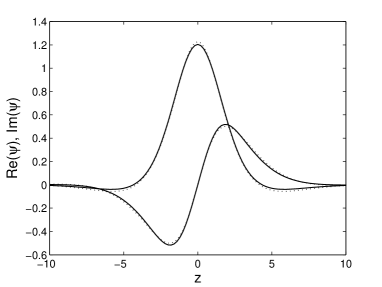
(a) $\varepsilon=1$, $c=0.7$, and $\Lambda=0.5$

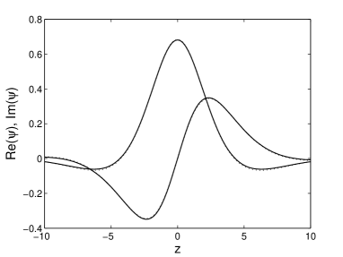
(b) $\varepsilon=1$, $c=0.7$, and $\Lambda=0.7$

Figure 1: The comparison of two soliton profiles for two different values of $\Lambda$, as indicated in the caption to each panel. The solid lines correspond to numerical results, i.e., solutions of Eq. (44) imposed with constraints (47), with $\Delta z=0.2$ and $L=50$ (the $z$-axis is truncated to focus the picture on the soliton’s core), both the real and imaginary parts being shown. The dotted lines are predictions of the variational approximation obtained through solving Eqs. (12)–(14).

For given parameters $\varepsilon,c$, and $\Lambda$, we solved variational equations (12)–(14) to produce suitable real solutions $A,a$ and $p$, which then give a quasi-analytical approximation for the soliton’s core described by function $\psi_{\mathrm{core}}(z)$ (see Eq. (8)). As generic examples, in Fig. 1 we present, at $\varepsilon=1$ and $c=0.7$, the comparison of two soliton profiles obtained from the numerical results and VA for two different values of $\Lambda$. We have found $A\approx 1.228,\,a\approx 0.554$, $p\approx 0.377$ for $\Lambda=0.5$ (Fig. 1(a)), and $A\approx 0.685,\,a\approx 0.414,$ $p\approx 0.368$ for $\Lambda=0.7$ (Fig. 1(b)). Particularly good agreement is observed in both cases.

To further confirm the agreement for different values of $\Lambda$, $\varepsilon$ and $c$, in the following we compare parameters $A,a$ and $p$ produced by the VA with their numerical counterparts. To calculate the latter, we make use of the following relations, which are generated by ansatz (8), (9) at $z=0$:

$$\psi(0)=A,\,\psi^{\prime}(0)=ipA,\,\psi^{\prime\prime}(0)=-A(a^{2}+p^{2}),$$ (48)

and take the left-hand sides of these relations from numerical data. Thus, using the central finite differences, we obtain the numerical counterparts of $A$, $p$, and $a$:

$$A_{\mathrm{num}} = \psi_{\frac{N+1}{2}},$$ (49)

$$p_{\mathrm{num}} = \frac{\mathrm{Im}\left(\psi_{\frac{N+1}{2}+1}\right)-\mathrm{Im}\left(\psi_{\frac{N+1}{2}-1}\right)}{2A\Delta z},$$ (50)

$$a_{\mathrm{num}} = \pm\sqrt{-\frac{\mathrm{Re}\left(\psi_{\frac{N+1}{2}-1}\right)-2\mathrm{Re}\left(\psi_{\frac{N+1}{2}}\right)+\mathrm{Re}\left(\psi_{\frac{N+1}{2}+1}\right)}{A_{\mathrm{num}}(\Delta z)^{2}}-p_{\mathrm{num}}^{2}}.$$ (51)

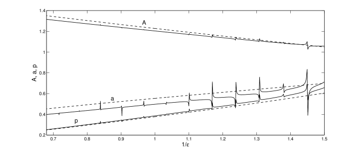
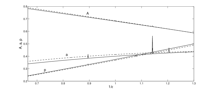
Figure 2: The comparison of parameters $(A,a,p)$ calculated from the numerical data (solid lines) through Eqs. (49)–(51), and from the VA (dashed lines) through Eqs. (48), for $c=0.7$ and $\Lambda=0.5$ (a) or $\Lambda=0.7$ (b) for varying $1/\varepsilon$.

The comparison of parameters $(A,a,p)$ obtained numerically (solid line) and from the VA (dashed line) is shown in Fig. 2 for varying $1/\varepsilon$ and fixed $(c,\Lambda)=(0.7,0.5)$. We observe that the solid and dashed curves are generally close for all the three parameters. Nevertheless, we also obtain isolated values of $1/\varepsilon$, which behave as singular points. Near the singularities the numerical results deviate very rapidly from the predictions of the VA. In fact, at these singular points the numerically obtained solutions are strongly delocalized due to the resonance of the oscillating tails with the finite size of the computational domains, hence the positions of such singularities depend on $L$, and they may be considered as artifacts of approximating the infinite region by the finite domain.

Similarly to Fig. 1, where a better approximation is obtained for larger $\Lambda$, we also observe in Fig. 2 that the variational and numerical curves for $A,\,a,\,p$ are closer for $\Lambda=0.7$ than those in 2. In the latter case, the singularities are present too, even though they are less pronounced here.

Thus we can conclude that the VA provides a reliable approximation for description of the soliton’s core.

3.2 Embedded solitons

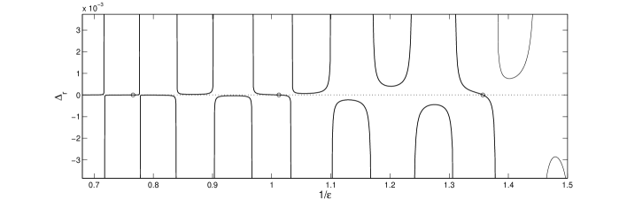
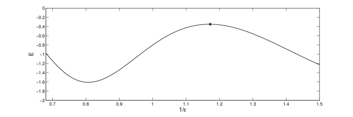
Figure 3: (a) The signed measure $\Delta_{r}$ (cf. Eq. (53)) as a function of $1/\varepsilon$ for $c=0.7$, $\Lambda=0.5$, $\Delta z=0.2$, and $L=50$, where $\Delta_{r}$ is zero at $\varepsilon\approx 0.737,0.988,1.306$ (or at $1/\varepsilon\approx 1.357,1.012,0.766$), as shown by empty circles. (b) $E$ versus $1/\varepsilon$ (cf. Eq. (23)), for the same parameter values $(\Lambda,c)$ as in panel (a) and for the corresponding solutions for $(A,a,p)$ and root(s) $\lambda$ obtained from the Eqs. (12)-(14) and Eq. (18), respectively. It is clearly seen that $E\neq 0$ in the observed domain of $1/\varepsilon$. However, we can conjecture that ESs are located near the maximum of $E$, i.e., at $\varepsilon\approx 0.853$ (or at $1/\varepsilon\approx 1.172$), as indicated by the star.

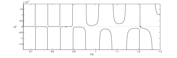
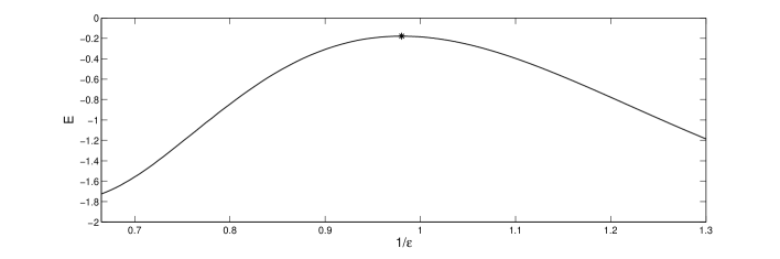
Figure 4: The same as Fig. 3, but for $\Lambda=0.7$. Zeros of $\Delta_{r}$ are found at $\varepsilon\approx 0.828,1.158$ (or at $1/\varepsilon\approx 1.2077,0.8636$), and the maximum of $E$ occurs at $\varepsilon\approx 1.020$ (or at $1/\varepsilon\approx 0.980$).

As shown in Ref. [21], in the general case the numerically obtained solitary waves are weakly delocalized, i.e., oscillatory tails with a nonvanishing amplitude are attached to them. Nevertheless, as suggested in Refs. [20, 21], it is possible to find solutions with vanishing tails (i.e., genuine solitons) by considering quantity

$$\Delta_{i}=\mathrm{Im}(\psi(N)),$$ (52)

which is a signed measure, whose zeros correspond to solutions with vanishing tails. In the present case, the periodic boundary conditions lead to $\mathrm{Im}(\psi(N))=0$, since the imaginary part of $\psi$ is odd. Therefore, we modify the signed measure (52) and redefine it as

$$\Delta_{r}=\mathrm{Re}(\psi(N)).$$ (53)

In Fig. 3 $\Delta_{r}$ is plotted as a function of $1/\varepsilon$ for the parameter values $(\Lambda,c,\Delta z,L)$ used in Fig. 2. We see from the figure that zeros of $\Delta_{r}$ occur at $\varepsilon\approx 0.737,0.988,1.306$ (i.e., at $1/\varepsilon\approx 1.357,1.012,0.766$). For the parameter values in Fig. 2, we show the corresponding $\Delta_{r}$ in Fig. 4, from which we conclude that $\Delta_{r}$ vanishes at $\varepsilon\approx 0.828,1.158$ (i.e., at $1/\varepsilon\approx 1.208,0.864$). It is worthy of note that the plot of $\Delta_{r}$ also has singularities which occur at exactly the same points as those in Fig. 2 obtained from the soliton’s core.

To predict the location of the ESs, we substitute the solution of Eqs. (12)–(14) and the root(s) $\lambda$ of Eq. (18) into Eqs. (23) to find $E$ as a function of $\varepsilon,c$, and $\Lambda$. Therefore, the existence of the ESs can be predicted by seeking for values of the parameters at which $E=0$. For the parameter values used in Figs. 3 and 4, curves for $E$ are displayed, respectively, in Figs. 3 and 4. It is seen that $E\neq 0$ in all the figures, i.e., truly localized solitons cannot be directly predicted by the VA.

However, we can propose a conjecture, based on a “phenomenological” consideration of the figures, that there are two zeros of $\Delta_{r}$ on the left and right of a maximum of $E$. For example, in Fig. 3 we have the maximum of $E$ at $\varepsilon\approx 0.853$ (i.e., at $1/\varepsilon\approx 1.172$), which is located between two adjacent numerically found zeros of $\Delta_{r}$. The same phenomenon also takes place in Fig. 4, where the two zero-crossing points lie between maxima of $E$, i.e., at $\varepsilon\approx 1.020$ (i.e., at $1/\varepsilon\approx 0.980$) in Fig. 4. We have also computed (not shown here) the signed measure $\Delta_{r}$ and $E$ for other combinations of parameter values, where we observed the same pattern. Thus, we conclude that, with addition of a constant, function $E$ may be able to predict the location of the ESs. We suspect that the missing constant, which amounts to the shift of the plot for $E$ vertically, is related to the choice of the ansatz (see, e.g., [40] for different ansätze accounting for the oscillating tails).

3.3 Stability

To determine the VA-predicted stability of the soliton, we have solved the eigenvalue problem (30). For the soliton shown in Fig. 1(a), i.e., with $\mathbf{x}_{0}\approx\left[1.228,0.554,0.377,0,0,0\right]^{T}$, we obtain the corresponding eigenvalues $\Omega\approx 0,0,0,0,0.436i,-0.436i$. In addition, for the soliton in Fig. 1(b), i.e., $\mathbf{x}_{0}\approx\left[0.685,0.414,0.368,0,0,0\right]^{T}$, the corresponding eigenvalues are $\Omega\approx 0,0,0,0,0.225i,-0.225i$. As the real part of all eigenvalues is zero, we conclude that both solitons are stable. These results are in agreement with the numerical findings of Ref. [21].

3.4 Bound states

Two examples of bound states consisting of two solitons, found numerically, are presented in Fig. 5, each for the same parameter values.

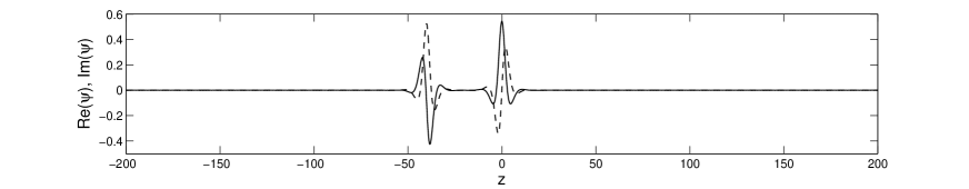
(a) $|l|\approx 39.6$

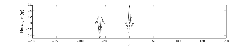
(b) $|l|\approx 60.87$

Figure 5: Two bound states, for $\varepsilon=0.7$, $c=0.7$, $\Lambda=0.7$, and $\Delta z=0.2$, found numerically in the interval of $[-200,200]$, for different distances between the two humps, $|l|$, as indicated in each panel. Solid and dashed lines depict $\text{Re}(\psi)$ and $\text{Im}(\psi)$, respectively.

Next, we compare the prediction presented above with the numerical results shown in Fig. 5. For the parameter values used in that figure, we have $\lambda_{r}\approx 0.441$ and $\lambda_{i}\approx 0.505$. Note that, in terms of the above analysis, the soliton centred at $z=0$ in Fig. 5 is in fact soliton No. 2. Therefore, phase difference $\phi$ in this case is calculated as the phase of the soliton on the right minus the phase of its counterpart on the left. From the numerical results, the phase difference between the two solitons shown in the top and the bottom panels of Fig. 5 is given, respectively, by $\phi\approx-2.012~{}$and $\phi\approx 2.368,$ both of which correspond to $c\lambda_{i}/\lambda_{r}>0$, hence $n\cdot\mathrm{sign}\left(\lambda_{i}\right)$ is odd. Using Eq. (43), we find that the best fit to the numerically computed distance in Fig. 5, i.e., $|l|\approx 39.6$ and $|l|\approx 60.87$, is provided by $l_{7}\approx 41.252$ and $l_{9}\approx 62.367$. Considering the fact that Eq. (43) is based on a simple approximation (Eqs. (36), (40) and (41)) and the assumption that the interacting solitons have decaying oscillating tails, the approximation is in relatively good accordance with the results provided by the numerical solution of the full equation.

Using the Runge–Kutta method, we have also carried out numerical integration of evolution equation (1), with initial conditions taken as in Fig. 5. The resulting evolution of the solutions is displayed in Fig. 6, where we see that both solitons maintain their shapes and positions for a relatively long time.

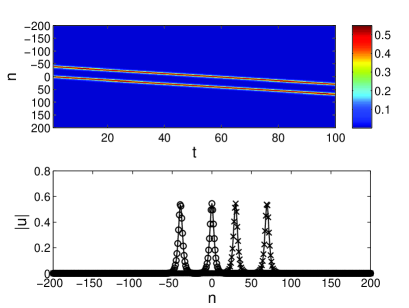
(a) $l\approx 39.6$

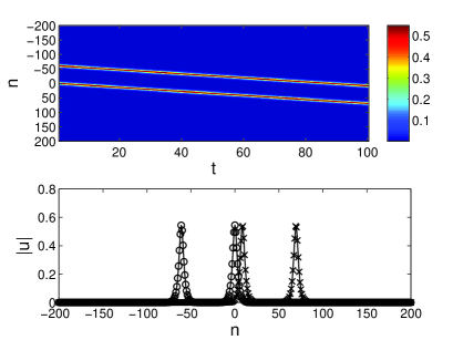
(b) $l\approx 60.87$

Figure 6: Numerical evolution of the solutions presented in Fig. 5, obtained by means of a numerical grid with 401 sites. Upper figures in each panel display the motion of the solution through the lattice for the first 100 time units. Shown is a spatiotemporal contour plot of the absolute value of the solution. Bottom figures in each panel depict the initial (open circles) and final (crosses) profiles of the absolute value of the solution after 100 time units of the evolution.

4 Conclusion

The aim of this work is to develop the semi-analytical approach to seeking travelling solitons, based on the application of the VA to the differential–difference form of the DNLSE with the saturable nonlinearity, in the moving coordinate frame. The predicted shapes of the solitons are in good agreement with the numerical findings. The VA is also extended to examine the stability of the travelling solitons, showing that they are stable, which is consistent with previous work [21]. Further, the VA was developed to predict the locations of the exceptional solutions for genuine travelling solitons with strictly vanishing tails. Bound states of two solitons were briefly considered too. In the latter case, the VA predicts the distance between two solitons forming the bound state. In the numerical part of the work, we have made use of the numerical scheme for the DNLSE written in the moving coordinate frame, which is an equation of the differential–difference type. Using the Newton–Raphson method, we have confirmed the existence of exceptional solutions for travelling discrete solitons (which are “embedded solitons”, in this sense), earlier predicted by means of a different numerical algorithm. We have compared the analytical results based on the VA and the numerical findings, concluding that they are in good agreement.

References

References

- [1] R. Peierls, The size of a dislocation, Proc. Phys. Soc. London 52, 34 (1940); F. R. N. Nabarro, Dislocations in a simple cubic lattice, ibid. 59, 256 (1947).
- [2] P. G. Kevrekidis (Editor), Discrete Nonlinear Schrödinger Equation: Mathematical Analysis, Numerical Computations and Physical Perspectives (Springer: New York, 2009).
- [3] F. Lederer, G. I. Stegeman, D. N. Christodoulides, G. Assanto, M. Segev, Y. Silberberg, Discrete solitons in optics, Phys. Rep. 463 (2008) 1-126; Y. V. Kartashov, V. A. Vysloukh, L. Torner, Soliton shape and mobility control in optical lattices, Progress in Optics 52 (2009) 63.
- [4] A. Smerzi, A. Trombettoni, Nonlinear tight-binding approximation for Bose-Einstein condensates in a lattice, Phys. Rev. A 68 (2003) 023613; R. Carretero-González, D. J. Frantzeskakis, P. G. Kevrekidis, Nonlinear waves in Bose–Einstein condensates: physical relevance and mathematical techniques, Nonlinearity 21 (2008) R139.
- [5] J. C. Eilbeck, Numerical simulations of the dynamics of polypeptide chains and proteins. In C. Kawabata and A. R. Bishop (Editors), Computer Analysis for Life Science: Progress and Challenges in Biological and Synthetic Polymer Research, pages 12-21 (Ohmsha: Tokyo, 1986).
- [6] H. Feddersen, Solitary wave solutions to the discrete nonlinear Schrödinger equation. In M. Remoissenet and M. Peyrard (Editors), Nonlinear Coherent Structures in Physics and Biology, vol. 393 of Lecture Notes in Physics, pages 159-167 (Springer: Berlin, 1991).
- [7] D. B. Duncan, J. C. Eilbeck, H. Feddersen, and J. A. D. Wattis, Solitons on lattices, Physica D 68 (1993) 1-11.
- [8] J. Gómez-Gardeñes, F. Falo, and L. M. Floría, Mobile localization in nonlinear Schrödinger lattices, Phys. Lett. A 332 (2004) 213; J. Gómez-Gardeñes, L. M. Floría, M. Peyrard, and A. R. Bishop, Nonintegrable Schrödinger discrete breathers, Chaos 14 (2004) 1130.
- [9] D. E. Pelinovsky, T. R. O. Melvin, and A. R. Champneys, One-parameter localized traveling waves in nonlinear Schrödinger lattices, Physica D 236 (2007) 22-43.
- [10] T. R. O. Melvin, A. R. Champneys, and D. E. Pelinovsky, Discrete traveling solitons in the Salerno model, SIAM J. Appl. Dyn. Syst. 8 (2009) 689-709.
- [11] J. W. Fleischer, M. Segev, N. K. Efremidis, D. N. Christodoulides, Observation of two-dimensional discrete solitons in optically induced nonlinear photonic lattices, Nature 422 (2003) 147.
- [12] D. Neshev, T. J. Alexander, E. A. Ostrovskaya, Y. S. Kivshar, H. Martin, I. Makasyuk, Z. Chen, Observation of discrete vortex solitons in optically induced photonic lattices, Phys. Rev. Lett. 92 (2004) 123903; J. W. Fleischer, G. Bartal, O. Cohen, O. Manela, M. Segev, J. Hudock, and D. N. Christodoulides, Observation of vortex-ring “discrete” solitons in 2D photonic lattices, Phys. Rev. Lett. 92 (2004) 123904.
- [13] J. Yang, I. Makasyuk, P. G. Kevrekidis, H. Martin, B. A. Malomed, D. J. Frantzeskakis, Z. G. Chen, Necklacelike solitons in optically induced photonic lattices, Phys. Rev. Lett. 94 (2005) 113902.
- [14] X. S. Wang, Z. G. Chen, P. G. Kevrekidis, Observation of discrete solitons and soliton rotation in optically induced periodic ring lattices, Phys. Rev. Lett. 96 (2006) 083904.
- [15] P. G. Kevrekidis, Z. G. Chen, B. A. Malomed, D. J. Frantzeskakis, M. I. Weinstein, Spontaneous symmetry breaking in photonic lattices: Theory and experiment, Phys. Lett. A 340 (2005) 275-280.
- [16] H. Sakaguchi, B. A. Malomed, Higher-order vortex solitons, multipoles, and supervortices on a square optical lattice, Europhys. Lett. 72 (2005) 698–704; P. G. Kevrekidis, H. Susanto, Z. Chen, High-order-mode soliton structures in two-dimensional lattices with defocusing nonlinearity, Phys. Rev. E 74 (2006) 066606.
- [17] R. Carretero-González, J. D. Talley, C. Chong, B. A. Malomed, Multistable solitons in the cubic–quintic discrete nonlinear Schrödinger equation, Physica D 216 (2006) 77–89; C. Chong, R. Carretero-González, B. A. Malomed, P. G. Kevrekidis, Multistable solitons in higher-dimensional cubic quintic nonlinear Schrödinger lattices, ibid. 238 (2009) 126-136.
- [18] R. A. Vicencio, M. Johansson, Discrete soliton mobility in two-dimensional waveguide arrays with saturable nonlinearity, Phys. Rev. E 73 (2006) 046602.
- [19] L. Hadžievski, A. Maluckov, M. Stepić, D. Kip, Power controlled soliton stability and steering in lattices with saturable nonlinearity, Phys. Rev. Lett. 93 (2004) 033901.
- [20] T. R. O. Melvin, A. R. Champneys, P. G. Kevrekidis, J. Cuevas, Radiationless travelling waves in saturable nonlinear Schrödinger lattices, Phys. Rev. Lett. 97 (2006) 124101.
- [21] T. R. O. Melvin, A. R. Champneys, P. G. Kevrekidis, J. Cuevas, Travelling solitary waves in the discrete Schrödinger equation with saturable nonlinearity: Existence, stability, and dynamics, Phys. D 237 (2008) 551-567.
- [22] J. Yang, B. A. Malomed, and D. J. Kaup, Embedded solitons in second-harmonic-generating systems, Phys. Rev. Lett. 83 (1999) 1958-1961; A. R. Champneys, B. A. Malomed, J. Yang, and D. J. Kaup. “Embedded solitons”: solitary waves in resonance with the linear spectrum, Physica D 152-153 (2001) 340-354.
- [23] A. R. Champneys and B. A. Malomed, Moving embedded solitons, J. Phys. A 32 (1999) L547-L553.
- [24] S. Gonzalez-Perez-Sandi, J. Fujioka, and B. A. Malomed, Embedded solitons in dynamical lattices, Physica D 197 (2004) 86-100; K. Yagasaki, A. R. Champneys, and B. A. Malomed, Discrete embedded solitons, Nonlinearity 18 (2005) 2591-2613; B. A. Malomed, J. Fujioka, A. Espinosa-Ceron, R. F. Rodriguez, and S. Gonzalez, Moving embedded lattice solitons, Chaos 16 (2006) 013112.
- [25] O. F. Oxtoby and I. V. Barashenkov, Moving solitons in the discrete nonlinear Schrödinger equation, Phys. Rev. E 76 (2007) 036603.
- [26] B. A. Malomed and M. I. Weinstein, Soliton dynamics in the discrete nonlinear Schrödinger equation, Phys. Lett. A 220 (1996) 91-96.
- [27] D. J. Kaup, Variational solutions for the discrete nonlinear Schrödinger equation, Math. Comput. Simulat., 69 (2005), 322-333.
- [28] C. Chong and D. E. Pelinovsky, Variational approximations of bifurcations of asymmetric solitons in cubic-quintic nonlinear Schrödinger lattices, Disc. Cont. Dyn. Sys. S 4 (2011) 1019-1032.
- [29] C. Chong, D. E. Pelinovsky and G. Schneider, On the validity of the variational approximation in discrete nonlinear Schrödinger equations, Physica D 241, 115-124 (2011).
- [30] D. J. Kaup and B. A. Malomed, Embedded solitons in Lagrangian and Semi-Lagrangian Systems, Physica D 184 (2003) 153-161.
- [31] I. S. Gradshteyn and I. M. Ryzhik, Tables of Integrals, Series, and Products (Academic Press: New York, 2000).
- [32] N. Flytzanis, B.A. Malomed, and J. A. D. Wattis, Analysis of stability of solitons in one-dimensional lattices, Phys. Lett. A 180 (1993) 107-112.
- [33] Y. S. Kivshar, A. R. Champneys, D. Cai, and A. R. Bishop, Multiple states of intrinsic localized modes, Phys. Rev. B 58 (1998) 5423-5428.
- [34] T. Kapitula, P. G. Kevrekidis, and B. A. Malomed, Stability of multiple pulses in discrete systems, Phys. Rev. E 63 (2001) 036604.
- [35] P. G. Kevrekidis, Multipulses in discrete Hamiltonian nonlinear systems, Phys. Rev. E 64 (2001) 026611.
- [36] B. A. Malomed and A. A. Nepomnyashchy, Stability limits for arrays of kinks in two-component nonlinear systems, Europhys. Lett. 27 (1994) 649.
- [37] B. A. Malomed, Potential of interaction between two- and three-dimensional solitons, Phys. Rev. E 58 (1998) 7928.
- [38] J. Weideman and S. Reddy, A MATLAB differentiation matrix suite, ACM Trans. Math. Software 26 (2000) 465–519.
- [39] L. N. Trefethen, Spectral Methods in MATLAB, (SIAM: Philadelphia, PA, 2000).
- [40] J. P. Boyd, Weakly nonlocal solitary waves and beyond-all-orders asymptotics, (Kluwer Academic Publishers: Dordrecht, 1998).