Fidelity for kicked atoms with gravity near a quantum resonance

Abstract

Kicked atoms under a constant Stark or gravity field are investigated for experimental setups with cold and ultra cold atoms. The parametric stability of the quantum dynamics is studied using the fidelity. In the case of a quantum resonance, it is shown that the behavior of the fidelity depends on arithmetic properties of the gravity parameter. Close to a quantum resonance, the long time asymptotics of the fidelity is studied by means of a pseudo-classical approximation first introduced by Fishman et al. [J. Stat. Phys. 110, 911 (2003)]. The long-time decay of fidelity arises from the tunneling out of pseudo-classical stable islands, and a simple ansatz is proposed which satisfactorily reproduces the main features observed in numerical simulations.

I Introduction

The stability of quantum evolution against parametric changes of the quantum Hamiltonian is a subject of wide theoretical and experimental interest. A widely used concept is the fidelity introduced by Peres peres , and the closely related Loschmidt echo JP2001 ; Gorin2006 , which is built as the interference pattern between states which are obtained by propagating the same initial state under Hamiltonians, say $\hat{H}_{0}$ and $\hat{H}$, which are slight perturbations of each other. A standard definition of the fidelity is:

$$F(t)=\left|\langle\psi|e^{\mathrm{i}\hat{H_{0}}t/\hbar}e^{-\mathrm{i}\hat{H}t/\hbar}|\psi\rangle\right|^{2}.$$ (1)

The behavior of fidelity in time is known to display some universal properties that reflect the underlying classical dynamics JP2001 ; Gorin2006 . Such properties have been mostly explored for the case of systems, which are chaotic in the classical limit. In this paper we will study the fidelity in the mixed phase space regime. For this the system under consideration is the quantum kicked rotor Casati ; chirikov ; raizen .

The main motivation for our analysis here is twofold. Firstly, there has been a growing interest over the last decade in the dynamics of the quantum kicked rotor (and its variants) at and close to the so-called quantum resonances QR , theoretically (see, e.g, fishman2002 ; sandro2003 ; sheinman ; kres ; italo2006 ; sandro06 ; italo2008 ; abb ; review ) as well as experimentally (see, e.g., oberthaler ; Gil2006 ; sadgrove ; nist ; sadgrove2007 ; harvard ; Gil2010 ). Secondly, only recently concepts have been developed to actually access the fidelity in setups based on cold or ultracold quantum gases. The used techniques range from interferometric methods in either internal atomic states exp or in the center-of-mass motion of the atoms harvard to the time reversal of the dynamics by exploiting the properties of the quantum resonant motion Gil2010 ; hoo2011 .

In this paper we study the quantum kicked rotor under the additional influence of a Stark or gravity field oberthaler ; fishman2002 . In Sect. II the Hamiltonian of one kicked atom is quickly reminded and the fidelity, which is the main quantity studied here, is precisely defined for our system. We then report on a subtle dependence of the fidelity on the arithmetic properties of the relevant parameters (Sect. III), a result which may be interesting for future precise measurements of fundamental constants (see the discussions in refs. harvard ; Gil2010 ; sack2011 ). Sect. IV is devoted to the dynamics close to quantum resonance. Based on the pseudo or $\epsilon-$classical formalism developed by Fishman et al. fishman2002 , we explain the overall behavior of the fidelity using $\epsilon-$classical phase space densities and quantum tunneling rates from the stable resonance island to the surrounding chaotic sea in phase space. Some technical details are found in appendices.

II The kicked rotor with gravity

We are interested in the quantum dynamics of a particle moving in a line, periodically kicked in time, and subject to a constant Stark or gravity field. It is described by the Hamiltonian in dimensionless variables (such that $\hbar=1$) fishman2002 :

$$\hat{H}(\hat{x},\hat{p},t)\;=\;\frac{\hat{p}^{2}}{2}-\frac{\eta}{\tau}\;\hat{x}+k\cos(\hat{x})\sum_{\verb+t+\in\mathbb{Z}}\delta(t-\verb+t+\tau)\ .$$ (2)

The kicking period is $\tau$, the kicking strength is $k$, and $\verb+t+$ is a discrete time variable that counts the number of kicks. The parameter $\eta$ yields the change in momentum produced by the constant field in one kicking period. In the accelerated frame of reference fishman2002 , the potential experienced by the particle is periodic in space and so the quasi-momentum $\beta$ is conserved by the evolution. With the chosen units, $\beta$ takes all values between $0$ and $1$. Using Bloch theory, the particle dynamics can then be identified with that of a family of quantum rotors, labelled by the values of $\beta$. For the $\beta$-rotor (i.e., the rotor in the family to which a given value $\beta$ of the quasi-momentum is affixed) the evolution from immediately after the $(\verb+t+-1)$-th kick to immediately after the $\verb+t+$-th kick is described by the unitary propagator fishman2002 :

$$\hat{\cal U}_{\beta,k,\eta}(\verb+t+)\;=\;e^{-\mathrm{i}k\cos(\hat{\theta})}\;e^{-\mathrm{i}\tau/2(\hat{\cal N}+\beta+\eta\verb+t++\eta/2)^{2}}\ ,$$ (3)

and the evolution operator over the first $\verb+t+$ kicks is:

$$\hat{\cal U}_{\beta,k,\eta}^{\verb+t+}\;\equiv\;\hat{\cal U}_{\beta,k,\eta}(\verb+t-1+)\;\hat{\cal U}_{\beta,k,\eta}(\verb+t-2+)\dots\hat{\cal U}_{\beta,k,\eta}(\verb+1+)\;\hat{\cal U}_{\beta,k,\eta}(\verb+0+)\,.$$ (4)

where $\hat{\cal N}$ is the momentum operator:

$$\hat{\cal N}=-\mathrm{i}\frac{\mathrm{d}}{\mathrm{d}\theta}\ ,$$

with periodic boundary conditions. The time-dependent Hamiltonian that generates the quantum evolution corresponding to (4) is then:

$$\hat{\cal H}({\hat{\cal N}},\hat{\theta},\beta,t)=\frac{1}{2}\left(\hat{\cal N}+\beta+\frac{\eta}{\tau}t\right)^{2}+k\cos(\hat{\theta})\sum_{\verb+t+\in\mathbb{Z}}\delta(t-\verb+t+\tau)\ .$$ (5)

We will study the fidelity that measures the stability of the evolution (4) with respect to changes of the parameter $k$. For a given $\beta$-rotor this fidelity is defined by:

$$F_{\beta}(k_{1},k_{2},\eta,\verb+t+)=\Big{|}\left<\hat{\cal U}_{\beta,k_{1},\eta}^{\verb+t+}\psi\Big{|}\hat{\cal U}_{\beta,k_{2},\eta}^{\verb+t+}\psi\right>\Big{|}^{2}\ ,$$ (6)

Moreover, having in mind experimental situations with cold atoms exp ; sandro2003 ; sadgrove ; review ; harvard , we will also consider the case when the initial state of the atomic cloud is an incoherent mixture of plane waves with a distribution $\rho(\beta)$ of the quasi-momentum. In this case the fidelity is given by sandro06 :

$$F(k_{1},k_{2},\eta,\verb+t+)=\bigg{|}\int_{0}^{1}\rho(\beta)\left<\hat{\cal U}_{\beta,k_{1},\eta}^{\verb+t+}\psi\Big{|}\hat{\cal U}_{\beta,k_{2},\eta}^{\verb+t+}\psi\right>\mathrm{d}\beta\bigg{|}^{2}$$ (7)

III Fidelity at a quantum resonance

In the gravity free case ($\eta=0$), Eq. (3) describes the standard Kicked-Rotor (KR) dynamics, and so-called KR resonances QR ; kres-1 ; kres occur whenever $\tau$ is commensurate to $2\pi$. Then, for special values of quasi-momentum $\beta$, the energy of the $\beta$-rotor asymptotically increases quadratically as $\verb+t+\to\infty$. In the presence of gravity, asymptotic quadratic growth of energy at certain values of $\beta$ is still possible dana07 . Here we study the behavior of fidelity in the presence of gravity and for the case of a main KR resonance, i.e., $\tau=2\pi l$ (with integer $l$). Denoting $\psi_{\beta}(\verb+t+)\equiv\hat{\cal U}_{\beta,k,\eta}^{\verb+t+}\psi_{\beta}(0)$, one may explicitly compute fishman2002 :

$$\left<\theta|\psi_{\beta}(\verb+t+)\right>=e^{-\mathrm{i}\alpha(\beta,\eta,\verb+t+)}e^{-\mathrm{i}kA(\theta,\beta,\eta,\verb+t+)}\bigl{<}\theta-\verb+t+(2\beta+1)\pi l-\pi l\eta\verb+t+^{2}\;\big{|}\;\psi_{\beta}(0)\bigr{>}\,$$ (8)

where $\alpha(\beta,\eta,\verb+t+)$ is a global phase, and

$$A(\theta,\beta,\verb+t+)=\sum_{r=0}^{\verb+t+-1}\cos\bigl{(}\theta-(2\beta+1)\pi l\;r-2\pi lr\eta\verb+t++\pi l\eta r^{2}\bigr{)}\ .$$ (9)

From now on we assume that the initial state is a plane wave: $\left|\psi_{\beta}(0)\right>=|n_{0}\rangle$, i.e.

$$\left<\theta|\psi_{\beta}(0)\right>=\left<\theta|n_{0}\right>=\frac{e^{\mathrm{i}n_{0}\theta}}{\sqrt{2\pi}}\ .$$ (10)

The fidelity is directly obtained from (8) using the method described in sandro06 . First write $A(\theta,\beta,\verb+t+)=\mathrm{Re}\ (e^{\mathrm{i}\theta}W_{\verb+t+})$ with

$$W_{\verb+t+}\equiv W_{\verb+t+}(\eta,\beta)=\sum_{r=0}^{\verb+t+-1}e^{-\mathrm{i}\pi l(2\beta+1)r}e^{-\mathrm{i}2\pi lr\eta\verb+t++\mathrm{i}\pi l\eta r^{2}}\ .$$ (11)

Then from (8) it follows that the wave function after the $\verb+t+$-th kick is given in momentum representation by:

$$\left<n\left|\;\hat{\cal U}_{\beta,k_{1},\eta}^{\verb+t+}\;\right|\psi\right>\; = \;e^{n\mathrm{i}\arg(W_{\verb+t+})}\frac{1}{2\pi}\int_{0}^{2\pi}e^{\mathrm{i}(n_{0}-n)\theta}e^{-\mathrm{i}k|W_{\verb+t+}|\cos\theta}\;d\theta$$ (12)

$$= \;e^{n\mathrm{i}\arg(W_{\verb+t+})}(-\mathrm{i})^{n_{0}-n}J_{n_{0}-n}(k|W_{\verb+t+}|)\,$$

where $J_{n_{0}-n}(.)$ is the Bessel function of order $n_{0}-n$. Using this along with the addition formula of Bessel functions, see e.g. 7.15.(31) in bateman2 , one finds:

$$\left<\hat{\cal U}_{\beta,k_{1},\eta}^{\verb+t+}\psi\Big{|}\hat{\cal U}_{\beta,k_{2},\eta}^{\verb+t+}\psi\right>=J_{0}(\Delta k|W_{\verb+t+}|)\ ,$$ (13)

where we defined the perturbation parameter $\Delta k=k_{2}-k_{1}$, and so the fidelity of a single $\beta-$rotor is given by:

$$F_{\beta}(k_{1},k_{2},\eta,\verb+t+)=\Big{|}J_{0}(\Delta k|W_{\verb+t+}|)\Big{|}^{2}\,.$$ (14)

III.1 Asymptotics of the fidelity for one single rotor

From Eqs. (12) and (14) it is clear that the long time asymptotics of the wave-packet propagation, and of the fidelity as well, are determined by the behavior of $|W_{\verb+t+}|$ as $\verb+t+\to\infty$. One may write:

$$W_{\verb+t+}\;=\;e^{i\Phi(\eta,\beta,\verb+t+)}\;\mathfrak{W}(\beta,\eta,\verb+t+)\;,$$ (15)

where $\Phi(\eta,\beta,\verb+t+)=-\pi l(2\beta+1+\eta\verb+t+)\verb+t+$, and $\mathfrak{W}(\eta,\beta,\verb+t+)$ is a quadratic Weyl sum:

$$\mathfrak{W}(\eta,\beta,\verb+t+)\;=\;\sum_{r=1}^{\verb+t+}e^{\mathrm{i}\pi l(2\beta+1)\;r}\;e^{\mathrm{i}\pi l\eta\;r^{2}}\,.$$ (16)

The asymptotic behavior of such sums as $\verb+t+\to\infty$ is known to depend on the arithmetic nature of the number $\eta$, i.e., on whether it is rational or irrational, and in the latter case on its Diophantine properties berry . First of all, as the behavior of Weyl sums may be quite erratic, we resort to the time-averaged fidelity defined by:

$$\left<F_{\beta}(k_{1},k_{2},\eta,\verb+t+)\right>_{T}\equiv\frac{1}{T}\sum_{\verb+t+=0}^{T-1}F_{\beta}(k_{1},k_{2},\eta,\verb+t+),\quad T\gg 1\,,$$ (17)

which has a smoother dependence on time than the original fidelity.

The easiest case is when $\eta$ is rational: $\eta=p/q$, with $p$ and $q$ mutually prime integers. In that case, setting $r=2jq+\nu$ in the sum (16) with $j$ a non negative integer and $0\leq\nu\leq 2q-1$, the sum may be rewritten in the form:

$$\mathfrak{W}(\eta,\beta,\verb+t+)\;=\;C(\eta,\beta,\verb+t+)\;B(\eta,\beta,\verb+t+)\;,$$

where

$$C(\eta,\beta,\verb+t+)\; = \;\sum\limits_{j=0}^{[\verb+t+,2q]}e^{-4i\pi l\beta jq}\;,$$

$$B(\eta,\beta,\verb+t+)\; = \;\sum\limits_{\nu=0}^{\{\verb+t+,2q\}}e^{i\pi l(2\beta+1)\nu}\;e^{i\pi l\nu^{2}p/q}\;,$$ (18)

having denoted by $[\verb+t+,2q]$ the integer part of $\verb+t+/(2q)$ and $\{\verb+t+,2q\}=\verb+t+$ mod$(2q)$. The factor $B(\eta,\beta,\verb+t+)$ is a periodic function of $\verb+t+$ with period $2q$. Explicit calculation of the sum on the right hand side of the 1st equation shows that $C(\eta,\beta,\verb+t+)$ is:

• quasi-periodic for $\beta$ irrational,

• periodic for $\beta$ rational and $2\beta q$ non-integer,

• linear, i.e. $C(\eta,\beta,\verb+t+)=\verb+t+$, when $2\beta q$ is an integer.

Such facts have the following implications on wave packet dynamics on the one hand and on the behavior of the fidelity on the other hand. Two cases have to be distinguished, according to whether $2\beta q$ is integer, or not. In the former case, a quantum resonance occurs. Indeed, using that $|W_{\verb+t+}|$ is equal to $\verb+t+$ times a periodic function of $\verb+t+$, from Eq. (12) and from the well-known asymptotics of the Bessel functions at large argument and fixed order, see e.g. 7.13.1 (3) in bateman2 :

$$J_{n}(x)\sim\sqrt{\frac{2}{\pi x}}\cos\left(x-\frac{n\pi}{2}-\frac{\pi}{4}\right),\quad x\to\infty\,,$$ (19)

we find that the probability in the $n$-th momentum eigenstate decays in time like $1/\verb+t+$. Hence the wave packet spreads linearly in time in momentum space, and the energy quadratically increases. Instead, if $2\beta q$ is not an integer then Eq. (12) shows that the amplitude of the evolving wave function in any momentum eigenstate oscillates quasi-periodically in time, so no unbounded spreading in momentum space occurs.

A similar reasoning based on Eqs. (14) and (17) shows that, for all nonresonant values of $\beta$, the time-averaged fidelity saturates to a nonzero value in the limit $T\to\infty$ (Fig. 1a). Instead, at resonance ($2\beta q=$integer) from Eqs. (14) , (19) (with $n=0$) and (17), the fidelity is seen to asymptotically decay to zero like $\log(T)/T$ (case $\beta=0.5$ in Fig. 1a).
The case of irrational $\eta$ is much more difficult, as the behavior of Gauss sums crucially depends on the Diophantine properties of $\eta$ berry . Here we limit ourselves to a heuristic analysis. For strongly irrational $\eta$ one may naively picture $W_{\verb+t+}$ as a sort of random walk in the complex plane, suggesting that $|W_{\verb+t+}|$ grows like $\sqrt{\verb+t+}$ in some average sense. Thanks to (14) and (19) an asymptotic decay of the average fidelity like $1/\sqrt{\verb+t+}$ is then expected. This is roughly numerically confirmed for the case when $\eta$ is equal to the golden ratio in Fig. 1b. However the actual decay displays strong fluctuations because it depends on the continued fraction expansion of $\eta$, notably large partial quotients in the latter may cause fidelity to behave as in cases of rational $\eta$ over significant time scales, e.g., for $\eta=\pi=[3,7,15,1,292,1,1,\dots]$ in Fig. 1b.

a)

b)

Figure 1: (Color online) Fidelity for the kicked rotor with gravity at the quantum resonance $\tau=2\pi$ for $k_{1}=0.8\pi$ and $k_{2}=0.7\pi$. The initial state is a plane wave with zero momentum $n_{0}=0$. Several choices of $\eta$ and $\beta$ are shown: a) $\eta=0.1$. Full black line: const.$/{t}$. Blue dashed line: $\beta=0.23$. Green double dot-dashed line: $\beta=0.499$. Red dot-dashed line: $\beta=0.5$. b) Full black line: const.$/\sqrt{t}$. Blue dashed line: $\eta=(\sqrt{5}-1)/2$ (the Golden Ratio), $\beta=0.23$. Green double dot-dashed line: $\eta=\pi$, $\beta=0.23$. Red dot-dashed line: $\eta=\pi$, $\beta=0.5$.

In order to mimic the experimental setups based on cold atoms exp ; sandro2003 ; sandro06 ; sadgrove ; harvard ; review , we consider the case when the initial state of the kicked atoms is an incoherent mixture of plane waves with a uniform density of $\beta$: $\rho(\beta)=1$. The expression (7) is computed as an average over a large number of randomly chosen values of $\beta$. The result does not vary significantly when the number of values of $\beta$ exceeds a few thousands. We observe a sharp difference in the asymptotic regime depending on whether $\eta$ is rational or not, see Fig. 2. We again show the time-averaged quantity:

$$\left<F(k_{1},k_{2},\eta,\verb+t+)\right>_{T}\equiv\frac{1}{T}\sum_{\verb+t+=0}^{T-1}F(k_{1},k_{2},\eta,\verb+t+)\,.$$ (20)

For rational values of $\eta$, the fidelity is observed to saturate towards a finite value. This is not surprising, because this is precisely the expected behavior for all values of $\beta$ in a set of full measure. On the contrary, the fidelity decays like $1/T$ for irrational $\eta$, see Fig. 2. This is roughly explained noting that, besides the decaying prefactor $\sim|W_{\verb+t+}|^{-1/2}$ in the asymptotics (19) (with $n=0$), one more mechanism of decay is introduced by ensemble averaging, which affects the rapidly oscillating part of the Bessel function.

Figure 2: (Color online) Fidelity for an ensemble of kicked rotors with gravity at $\tau=2\pi$ for $k_{1}=0.8\pi$ and $k_{2}=0.7\pi$. The initial state is a plane wave with $n_{0}=0$. Several choices of $\eta$ are shown. The integral over $\beta$ in Eq. (7) is computed via a Riemannian sum with $5000$ randomly chosen $\beta$s. Full black line: const.$/t$. Blue dashed line: $\eta=$Golden Ratio. Green double dot-dashed line: $\eta=\pi$. Red dot-dashed line: $\eta=0.1$.

The observation of the fine details of the number theoretical properties of $\eta$ is certainly of high interest for precision measurements Gil2010 ; harvard ; hoo2011 ; sack2011 but, at the same time, a big challenge to experimental resolution in current setups.

IV Fidelity close to a quantum resonance.

IV.1 Reminder of the $\epsilon$-semiclassics. Fixed points.

When the kicking period is close to a quantum resonance,

$$\tau=2\pi l+\epsilon,\qquad l\textrm{ integer },|\epsilon|\ll 1,$$ (21)

we will implement a technique of quasi-classical approximation originally described in fishman2002 and therein termed “$\epsilon$-classical approximation”. Introducing a rescaled kick strength $\tilde{k}=|\epsilon|k$, and a new momentum operator

$$\hat{I}=|\epsilon|\hat{\cal N}=-\mathrm{i}|\epsilon|\frac{\mathrm{d}}{\mathrm{d}\theta}\,,$$ (22)

the propagator (3) may be rewritten as:

$$\hat{\cal U}_{\beta,k,\eta}(\verb+t+)=\exp\left(-\frac{\mathrm{i}}{|\epsilon|}\tilde{k}\cos(\hat{\theta})\right)\exp\left(-\frac{\mathrm{i}}{|\epsilon|}{\hat{\cal H}}_{\beta}(\hat{I},\verb+t+)\right)\ ,$$ (23)

where:

$$\hat{\cal H}_{\beta}(\hat{I},\verb+t+)\;=\;\frac{1}{2}\mathrm{sgn}(\epsilon){\hat{I}^{2}}\;+\;\hat{I}\bigl{[}\pi l+\tau(\beta+\eta\verb+t++\frac{\eta}{2})\bigr{]}.$$ (24)

The small parameter $\epsilon$ plays the formal role of a Planck constant in (23), so, close to a quantum resonance, the quantum dynamics mirrors an “$\epsilon$-classical” dynamics, which is immediately inferred from (23) and (24). After changing the $\epsilon$-classical momentum variable from $I$ to $J$ given by:

$${J}={I}+\mathrm{sgn}(\epsilon)[\pi l+\tau\beta+\tau\eta\verb+t++\tau\eta/2]\ ,$$ (25)

the $\epsilon$-classical dynamics is described by the following map that relates the variables $J$ and $\theta$ from immediately after the $\verb+t+$-th kick to immediately after the $(\verb+t++1)$-th one:

$$\left\{\begin{array}[]{rcl}J_{\verb+t++1}&=&J_{\verb+t+}\;+\;\tilde{k}\sin(\theta_{\verb+t++1})\;+\;\mathrm{sgn}(\epsilon)\tau\eta\\ \theta_{\verb+t++1}&=&\theta_{\verb+t+}\;+\;\mathrm{sgn}(\epsilon)J_{\verb+t+}\;\;\;\textrm{ mod }2\pi\end{array}\right.$$ (26)

If considered on the 2-torus, this map (26) has a fixed point at $J=0$ and $\theta=\theta_{0}$ if:

$$\sin\theta_{0}=-\mathrm{sgn}(\epsilon)\frac{\tau\eta}{\tilde{k}}\;,$$ (27)

and this fixed point is stable if and only if:

$$0\leq\tilde{k}|\cos\theta_{0}|\leq 4\quad\textrm{ and }\quad\cos\theta_{0}=-\mathrm{sgn}(\epsilon)|\cos\theta_{0}|\;.$$ (28)

Such stable fixed points give rise to stable islands immersed in a chaotic sea. From (25) it is immediately seen that, in physical momentum space, such islands travel at constant velocity:

$$v=-\frac{\tau\eta}{\epsilon}\;.$$ (29)

As islands trap some of the particle’s wave packet, they give rise to experimentally observable quantum accelerator modes oberthaler ; Gil2006 . Because of such modes a quadratic growth of energy is observed over significant time scales, both in the falling frame and in the laboratory frame fishman2002 . However such quadratic growth eventually comes to an end as the modes decay, due to tunneling out of the stable islands sheinman . Smaller accelerating islands may also exist, associated with higher-order fixed points of map (26) italo2006 ; italo2008 , however we will restrict ourselves to the above described ones.

IV.2 Long time asymptotics of the fidelity

Typical numerical results illustrating the time dependence of fidelity (6) are shown in Figs. 3–6. In all those simulations the parameters were chosen in ranges where significant, experimentally detectable accelerator modes exist (see Appendix A for details). In general, a very short initial transient is observed (typically up to one or a few hundred kicks depending on parameters), marked by a very quick drop. A clear, relatively long exponential decay follows. This is sometimes followed by yet another stage of exponential decay, at a slower rate and with stronger fluctuations. This general behavior is qualitatively understood as follows. The initial sharp decay is due to the part of the initial wave packet that lies in the chaotic component of either of the two dynamics (defined by the two different kick strengths), and is rapidly carried away. The fidelity is thereafter dominated by the parts of the wave packet which are trapped inside the islands. For this reason, in order to bring this stage of fidelity decay into full light, we choose our initial state in the form of a Gaussian state mostly located inside one island. The islands which correspond to the $k_{1}$ and to the $k_{2}$ dynamics are slightly displaced with respect to each other, however they travel in momentum space with the same velocity (29). Therefore, the mismatch between the $k_{1}$ and the $k_{2}$ dynamics is, in $\epsilon$-classical terms, mostly produced by (i) different structures inside the islands and (ii) the decay from the islands into the chaotic sea due to dynamical tunneling. Concerning (i), the different rotational frequencies in the two islands are expected to produce quasi-periodic oscillations of the fidelity abb ; ott_fishman2011 , so (ii) should be the main mechanism responsible of the mean fidelity decay. This leads to the following crude description. The main contribution to fidelity comes from the part of each factor in the scalar product in (6) which is trapped in the respective travelling island. Hence the decay of fidelity is determined by the decay of each part, which is in turn determined by its respective tunneling rate into the chaotic sea, which we will denote by $\Gamma_{i}$ for $i=1,2$. Then a simple, self-explanatory ansatz for the asymptotic decay of fidelity is

$$F(\verb+t+)\;\propto\;{\mu({\cal A}_{1}\backslash{\cal A}_{2})\;e^{-\Gamma_{1}\verb+t+}+\mu({\cal A}_{2}\backslash{\cal A}_{1})\;e^{-\Gamma_{2}\verb+t+}+\mu({\cal A}_{2}\cap{\cal A}_{1})\;e^{-(\Gamma_{1}+\Gamma_{2})\verb+t+}}\ ,$$ (30)

where $\mu$ is the classical invariant measure of phase space sets, ${\cal A}_{i}$ is the island around the fixed point associated with $k_{i}$. This ansatz was found to satisfactorily reproduce the actual decay of fidelity in our numerical checks. In our simulations, the phase-space areas appearing in (30) were estimated as described in appendix B. Quantum decay rates were found as follows: for both the $k_{1}$ and the $k_{2}$ dynamics we numerically computed the probability in a momentum range centered on the accelerator mode. This measures the amount of the initial probability, which travels within the accelerator mode. This quantity is called the survival probability and shown in Fig. 3. Fitting the long time decay of this probability with an exponential function gives us an estimate of the tunneling rate, see an example in Fig. 3. In our numerical simulations we take the following momentum range:

$$[n(\verb+t+)-15\;,\;n(\verb+t+)+15],\qquad n(\verb+t+)=n_{0}+v\verb+t+\ ,$$ (31)

where $n_{0}$ and $v$ are given respectively by (34) and (29). We checked that the peak traveling ballistically has a width less than $30$ (in two photonic recoil units for the experiment, see, e.g., review ) with our choice of parameters.

Figure 3: (Color online) Comparison between the survival probability (black and blue dashed lines) and the fidelity (red full line). $\tau=5.86$, $\epsilon=\tau-2\pi$, $\eta=0.01579\tau$, $\beta=0.48984326$, $k_{2}=0.8\pi$, $k_{1}=0.7\pi$. The upper blue dashed line corresponds to $k_{1}$ and gives the tunneling rates $\Gamma_{1}=5.1\times 10^{-4}$ whereas the lower black dashed line corresponds to $k_{2}$ and gives $\Gamma_{2}=4.4\times 10^{-5}$. The dot-dashed line corresponds to an exponential fit with a decay rate $\Gamma=3.5\times 10^{-5}$.

We note that the right hand side in Eq. (30) is defined up to a proportionality factor. Moreover, it crucially depends on $k_{1}$ and $k_{2}$, because island sizes and tunneling rates vary when the kicking strength is changed. In our simulations the proportionality factor was chosen such as to fit the earlier regime of exponential decay (approximately between 100 and $10^{4}$ kicks in Fig. 3 for instance). In our numerical computations the initial state is given by (33) with a width $\sigma^{2}=0.25$. As the fidelity is a wildly oscillating function, it is averaged over 200 kicks in order to clearly expose the mean long time behavior. Results are shown in the Figs. 4,5, and 6 for different sets of parameters and will be discussed in the following.

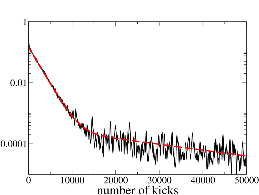
a)

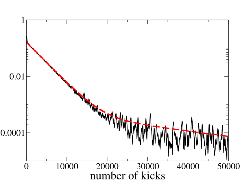
b)

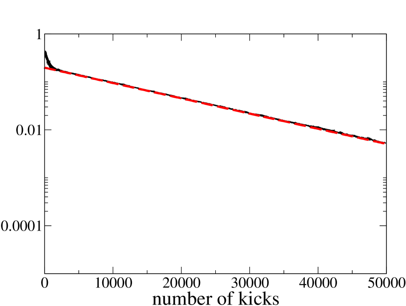
c)

Figure 4: (Color online) Comparison between the ansatz Eq. (30) (red dashed line) and the smoothed fidelity (black solid line) at $\tau=5.86$, $\epsilon=\tau-2\pi$, $\eta=0.01579\tau$, $\beta=0.48984326$, $k_{2}=0.8\pi$ and a) $k_{1}=0.7\pi$, b) $k_{1}=0.72\pi$, c) $k_{1}=0.83\pi$.

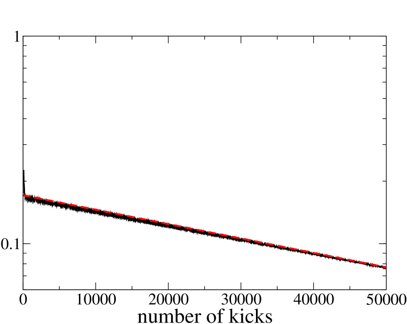
a)

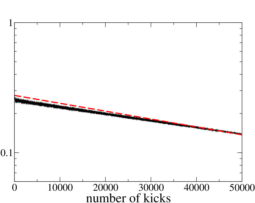
b)

Figure 5: (Color online) Same as in Fig. 4 at $\tau=6.6$, $\epsilon=\tau-2\pi$, $\eta=(\sqrt{5}-1)/20$, $\beta=0.123456789$, $k_{2}=2.5+\tau\eta$ and a) $k_{1}=2+\tau\eta$, b) $k_{1}=3.5+\tau\eta$.

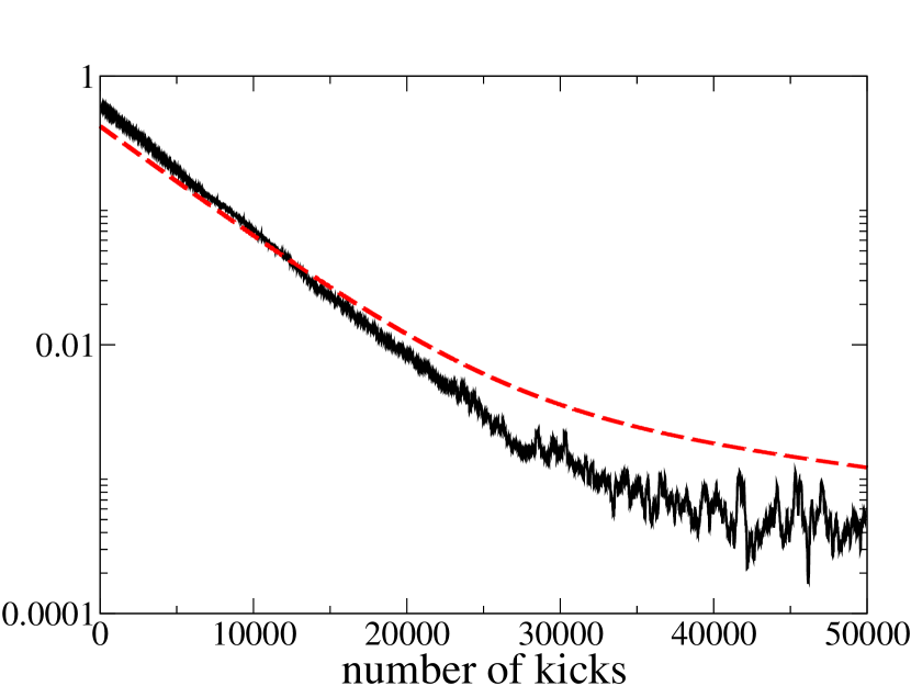
a)

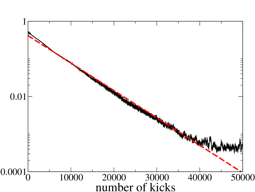
b)

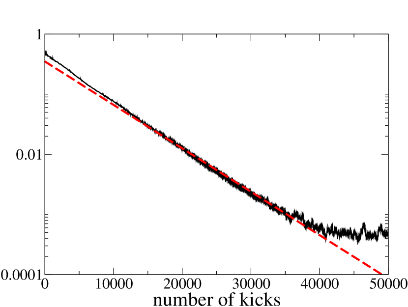
c)

Figure 6: (Color online) Same as Fig. 4 at $\epsilon=-0.5$, $\tau=4\pi+\epsilon$, $\eta=0.001$, $\beta=0.123456789$, $k_{2}=(1.35+\tau\eta)/|\epsilon|$ and a) $k_{1}=(1+\tau\eta)/|\epsilon|$, b) $k_{1}=(2+\tau\eta)/|\epsilon|$, c) $k_{1}=(2.2+\tau\eta)/|\epsilon|$.

The mean behavior of the fidelity for long times is well reproduced by the ansatz (30) when $\Gamma_{1}$ and $\Gamma_{2}$ are quite different: then the fidelity shows successively two different decay regimes, which are well reproduced by the pseudo-classical ansatz (30), see Figs. 4a ($\Gamma_{1}\simeq 10\Gamma_{2}$) and 4b ($\Gamma_{1}\simeq 5\Gamma_{2}$). On the contrary, when $\Gamma_{1}$ and $\Gamma_{2}$ are close to each other, one can see only one decay, which is still well reproduced by (30), see Fig. 4 ($\Gamma_{1}\simeq\Gamma_{2}$) and Fig. 5 ($\Gamma_{1}\simeq 3\Gamma_{2}$). For sake of comparison we are showing the same plots for $l=2$ in Fig. 6. The quantum resonance is then $\tau=4\pi$. It can be seen that the agreement is not so good in the latter case. One reason for this may be that higher order $\epsilon-$classical phase space structures have a larger area hence may play a more important role, making estimates of the various areas in (30) more problematic. Both $\epsilon-$classical phase spaces corresponding to $k_{1}$ and $k_{2}$ are displayed in Fig. 7 corresponding to Fig. 4a and Fig. 6c. It is clear that the shape and the overlap between the two islands are qualitatively different in these two situations.

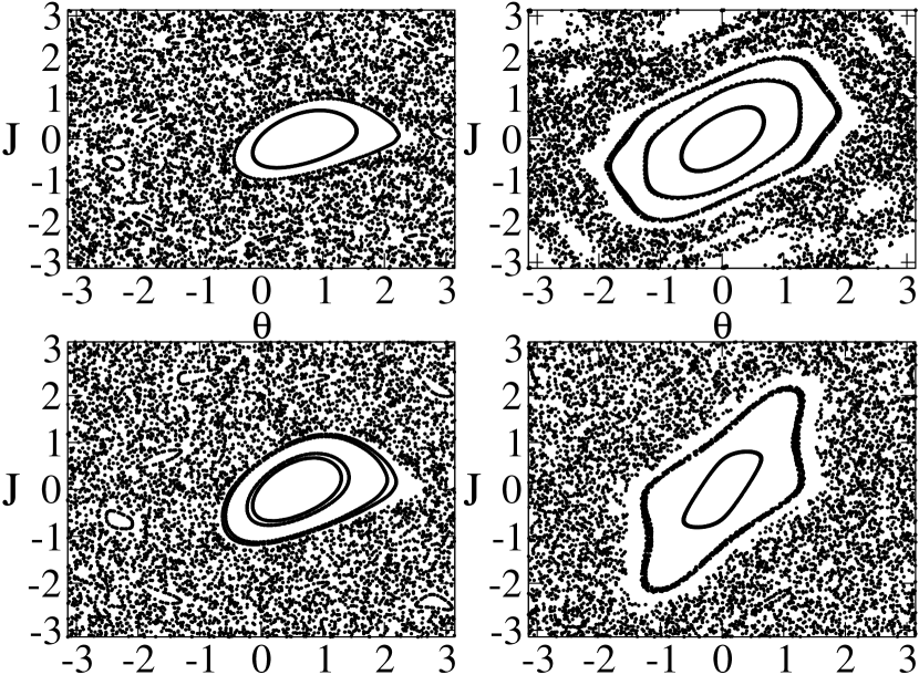
Figure 7: Phase spaces corresponding to two sets of parameters. Left column: $\tau=5.86$, $\epsilon=\tau-2\pi$, $\eta=0.01579\tau$. Top left: $k=0.7\pi$. Bottom left: $k=0.8\pi$. Right column: $\epsilon=-0.5$, $\tau=4\pi+\epsilon$, $\eta=0.001$. Top right: $k=(1.35+\tau\eta)/|\epsilon|$. Bottom right: $k=(2.2+\tau\eta)/|\epsilon|$.

V Conclusion

We have presented a theoretical analysis of the temporal dependence of fidelity for the quantum kicked rotor subject to an additional gravity field. The two major results concern the dynamics of this system at principal quantum resonances, i.e., at kicking periods $\tau=2\pi l$ ($l$ integer), and close to these resonances. In the former case, we arrive at analytical estimates for the decay of fidelity which is highly sensitive to the arithmetic properties of the gravity parameter. Close to a resonance we have used the $\epsilon-$semiclassical method in order to describe the long time asymptotics of the fidelity. The ansatz (30) based on semiclassical densities gives a good description of the long time behavior of the quantum fidelity for both similar and different tunneling rates of the two compared non-dispersive wave packets buch centered at the accelerator mode islands in phase space sheinman . This result highlights once more the utility of $\epsilon-$classics in describing the quantum evolution of the kicked rotor and its variants.

Appendix A Relevant range for the parameters.

It was observed numerically, when plotting the $\epsilon-$classical phase portrait, that higher order nonlinear resonances play a bigger role when $l$ is increased. For this reason we restrict in this paper mainly to $l=1$. In the experiments, see e.g. exp , $k$ typically runs from $0.3\pi\sim 0.94$ to $1.5\pi\sim 4.71$. In order to see an accelerator mode one needs a stable fixed point of the classical map. Following (27), for a given $k$ one has a fixed point when $\tilde{k}\geq\tau\eta$. Taking into account experimental constraints leads us to choose $\epsilon$ such that:

$$0.4<|\epsilon|<1\,.$$ (32)

For the quantum fidelity the initial state is chosen to be a Gaussian state:

$$\left<n|\psi_{\beta}(0)\right>=\frac{e^{-(n-n_{0})^{2}/4\sigma^{2}+\mathrm{i}n\theta_{0}}}{(2\pi\sigma^{2})^{1/4}}\ ,$$ (33)

with

$$\sin\theta_{0}=-\frac{\tau\eta}{\epsilon k},\quad n_{0}=\frac{2\pi\ m}{|\epsilon|}-\frac{1}{\epsilon}\left[\pi l+\tau\left(\beta+\frac{\eta}{2}\right)\right]\,,$$ (34)

where $m$ is an arbitrary integer. This initial state is centered on an accelerator mode for which $J=0$. This mode is travelling (in momentum space) at the speed (29), see e.g. fishman2002 . The fidelity is computed by applying successively the operators (3) for two different values of the kicking strength: $k_{1}$ and $k_{2}$. For each set of parameters we keep $k_{2}$ fixed and vary $k_{1}$. Our initial state is always chosen such as to follow the accelerator mode attached to $k_{1}$: once $\tau$ (and $\epsilon$), $\eta$ and $\beta$ are fixed, the initial state is centered in momentum space around $n_{0}$ defined by (34).

Appendix B Estimating the size of the islands in the $\epsilon-$classical phase space

First we choose a set of parameters $\tau$ and $\eta$ for which we can have accelerator modes. Then we vary $k$ within the range of existence of these modes. One way to see this range is to compute numerically the area of the stable island in the $\epsilon-$classical phase space, see Fig. 8.

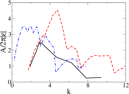
Figure 8: (Color online) Area of the stable island in the $\epsilon-$classical phase space as a function of the kicking strength for three sets of parameters. Black full line: $\tau=5.86,\epsilon=\tau-2\pi\sim-0.42,\eta=0.01579\tau$. Red dashed line: $\tau=6.6,\epsilon=\tau-2\pi\sim 0.32,\eta=\phi/10$. Blue dash-dotted line: $\epsilon=-0.5,\tau=4\pi+\epsilon,\eta=0.001$.

The area follows a bell shape as a function of $k$. In Fig. 8 some jumps are also visible (see e.g. for the blue dash-dotted line, between $k\simeq 4.424$ and $k\simeq 4.624)$. We believe that this is due to the lack of precision when determining the island boundary and/or the breaking of outermost tori and their remnants (cantori). The size of the stable island in the $\epsilon-$classical phase space is computed by starting a fairly small number of trajectories outside the island. These are typically iterated for a long time ($10^{8}$ kicks). Then we move to polar coordinates $(\varphi,I)$ centered at the fixed point under interest peter . The boundary of the island is then determined by the curve $I(\varphi)$ defined in the following way. Using a grid of thickness $\delta\varphi$ along the $\varphi$ axis, the boundary $I_{i}=I(\varphi_{i})$ is given by:

$$I_{i}=\min\left\{I_{j},(\varphi_{j},I_{j})\textrm{ iterated points and }\varphi_{i}\leq\varphi_{j}\leq\varphi_{i}+\delta\varphi\right\}$$ (35)

The size of the island is given by the area under this curve. Numerically it is computed via a Riemannian sum.
The measures of the different sets in (30) are computed by propagating a cloud of $10^{4}$ classical points. The initial points are distributed following normal distributions with mean and width $(\theta_{0},\sigma_{\theta})$ in the $\theta$ direction and $(J_{0},\sigma_{J})$ in the $J$ direction. The areas in (30) reached stationary values after ca $500$ kicks. The measures needed in (30) are simply given by the number of points sitting on one or both of the stable islands associated to $k_{1}$ and $k_{2}$, respectively.

References

- (1) A. Peres, Phys. Rev. A30, 1610 (1984).
- (2) R. A. Jalabert and H. M. Pastawski, Phys. Rev. Lett. 86, 2490 (2001).
- (3) T. Gorin, T. Prosen, T. H. Seligman, and M. Znidaric, Phys. Rep. 435, 33 (2006); P. Jacquod and C. Petitjean, Adv. Phys. 58, 67 (2009).
- (4) G. Casati et. al., in Stochastic Behavior in Classical and Quantum Hamiltonian Systems, ed. by G. Casati and J. Ford (Springer, Berlin, 1979), p. 334.
- (5) B. V. Chirikov, Phys. Rep. 52, 263 (1979).
- (6) F. L. Moore, J. C. Robinson, C. F. Bharucha, B. Sundaram and M. G. Raizen, Phys. Rev. Lett. 75, 4598 (1995); C. F. Bharucha, J. C. Robinson, F. L. Moore, B. Sundaram, Q. Niu, and M. G. Raizen, Phys. Rev. E60, 3881 (1999).
- (7) F. M. Izrailev and D. L. Shepelyanskii, Sov. Phys. Dokl. 24, 996 (1979, in Russian) transl. in Theoretical and Mathematical Physics 43, 553 (1980).
- (8) S. Fishman, I. Guarneri, L. Rebuzzini, Phys. Rev. Lett. 89, 084101 (2002); J. Stat. Phys. 110, 911 (2003).
- (9) S. Wimberger, I. Guarneri, and S. Fishman, Nonlinearity 16, 1381 (2003); Phys. Rev. Lett. 92, 084102 (2004).
- (10) M. Abb, I. Guarneri, and S. Wimberger, Phys. Rev. E80, 035206(R) (2009).
- (11) M. Sadgrove and S. Wimberger, A pseudo-classical method for the atom-optics kicked rotor: from theory to experiment and back, Adv. At. Mol. Opt. Phys. 60, 315 (2011, Elsevier, Amsterdam).
- (12) S. Wimberger and A. Buchleitner, J. Phys. B 39, L145 (2006).
- (13) I. Dana and D. L. Dorofeev, Phys. Rev. E73, 026206 (2006); I. Guarneri, Ann. Henri Poincaré 10, 1097 (2009).
- (14) I. Guarneri and L. Rebuzzini, S. Fishman, Nonlinearity 19, 1141 (2006).
- (15) I. Guarneri and L. Rebuzzini, Phys. Rev. Lett. 100, 234103 (2008).
- (16) M. Sheinman, S. Fishman, I. Guarneri, and L. Rebuzzini, Phys. Rev. A73, 052110 (2006).
- (17) M. K. Oberthaler, R. M. Godun, M. B. d’Arcy, G. S. Summy, and K. Burnett, Phys. Rev. Lett. 83, 4447 (1999); M. B. d’Arcy, R. M. Godun, M. K. Oberthaler, G. S. Summy, K. Burnett, and S. A. Gardiner, Phys. Rev. E64, 056233 (2001).
- (18) M. Sadgrove, S. Wimberger, S. Parkins, and R. Leonhardt, Phys. Rev. Lett. 94, 174103 (2005); Phys. Rev. A71, 053404 (2005); Phys. Rev. E78, 025206(R) (2008).
- (19) M. Sadgrove, M. Horikoshi, T. Sekimura, K. Nakagawa, Phys. Rev. Lett. 99, 043002 (2007); M. Sadgrove and S. Wimberger, New J. Phys. 11, 083027 (2009).
- (20) G. Behinaein, V. Ramareddy, P. Ahmadi, and G. S. Summy, Phys. Rev. Lett. 97, 244101 (2006).
- (21) I. Talukdar, R. Shrestha, and G. S. Summy, Phys. Rev. Lett. 105, 054103 (2010).
- (22) C. Ryu, M. F. Andersen, A. Vaziri, M. B. d’Arcy, J. M. Grossman, K. Helmerson, and W. D. Phillips, Phys. Rev. Lett. 96, 160403 (2006).
- (23) S. Wu, A. Tonyushkin, and M. G. Prentiss, Phys. Rev. Lett. 103, 034101 (2009); A. Tonyushkin, S. Wu, and M. G. Prentiss, Phys. Rev. A 79, 051402(R) (2009).
- (24) S. Schlunk, M. B. d’Arcy, S. A. Gardiner, D. Cassettari, R. M. Godun, and G. S. Summy, Phys. Rev. Lett. 90, 054101 (2003).
- (25) A. Ullah and M. D. Hoogerland, Phys. Rev. E83, 046218 (2011).
- (26) R. A. Horne, R. H. Leonard, and C. A. Sackett, Phys. Rev. A83, 063613 (2011).
- (27) S.-J. Chang and K.-J. Shi, Phys. Rev. A34, 7 (1986)
- (28) I. Dana and V. Roitberg, Phys. Rev. E76 , 015201(R) (2007).
- (29) Erdelyi et al., Higher Transcendental functions, Vol. 2, Mc Graw-Hill (1955).
- (30) G. H. Hardy and J. E. Littlewood, Acta Math. 37, 193 (1914); J. H. Hannay and M. V. Berry, Physica D 1, 267 (1980); M. V. Berry, J. Goldberg, Nonlinearity 1, 1 (1988); J. Marklof, Duke Math. J. 97, 127 (1999).
- (31) Y. Krivolapov, S. Fishman, E. Ott and T. M. Antonsen Phys. Rev. E83, 016204 (2011)
- (32) A. Buchleitner, D. Delande, and J. Zakrzewski, Phys. Rep. 368, 409 (2002); S. Wimberger, P. Schlagheck, Ch. Eltschka, and A. Buchleitner, Phys. Rev. Lett. 97, 043001 (2006).
- (33) P. Schlagheck, private discussion.