Physics of the Galactic Center Cloud G2, on its Way towards the Super-Massive Black Hole

Abstract

The origin, structure and evolution of the small gas cloud, G2, is investigated, that is on an orbit almost straight into the Galactic central supermassive black hole (SMBH). G2 is a sensitive probe of the hot accretion zone of Sgr A^∗, requiring gas temperatures and densities that agree well with models of captured shock-heated stellar winds. Its mass is equal to the critical mass below which cold clumps would be destroyed quickly by evaporation. Its mass is also constrained by the fact that at apocenter its sound crossing timescale was equal to its orbital timescale. Our numerical simulations show that the observed structure and evolution of G2 can be well reproduced if it formed in pressure equilibrium with the surrounding in 1995 at a distance from the SMBH of 7.6 $\times 10^{16}$ cm. If the cloud would have formed at apocenter in the ’clockwise’ stellar disk as expected from its orbit, it would be torn into a very elongated spaghetti-like filament by 2011 which is not observed. This problem can be solved if G2 is the head of a larger, shell-like structure that formed at apocenter. Our numerical simulations show that this scenario explains not only G2’s observed kinematical and geometrical properties but also the Br$\gamma$ observations of a low surface brightness gas tail that trails the cloud. In 2013, while passing the SMBH G2 will break up into a string of droplets that within the next 30 years mix with the surrounding hot gas and trigger cycles of AGN activity.

1 INTRODUCTION

The Galactic center is one of the most extreme and puzzling places of the Milky Way. Harboring a supermassive black hole (SMBH) with a mass of M${}_{BH}=4.31\times 10^{6}$ M_⊙ (Ghez et al. 2008; Gillessen et al. 2009, Genzel, Eisenhauer & Gillessen 2010) at the position of the radio source Sgr A^∗ it is by far the closest and most ideal place to investigate the physics of galactic nuclei and their activity cycles when gas accretes onto the SMBH. Most galaxies contain SMBHs that correlate well with various global galactic properties (Gültekin et al. 2009; Burkert & Tremaine 2010; Kormendy, Bender & Cornell 2011). However, only a small fraction is observed to be active at any time (e.g. Heckmann et al. 2004, King & Pringle 2007). The processes that lead to these long phases of quiescence with no or little SMBH accretion, interrupted by short periods of activity, are not well understood up to now.

The Milky Way’s central SMBH currently is classified as inactive, despite observations of irregular flickering events (Baganoff et al. 2001; Genzel et al 2003) that demonstrate that it is still accreting small amounts of mass, sporadically. The ’X-ray echo’ in the molecular clouds near Sgr A^∗ might be a signature of such an accretion event that occured a few hundred years ago with an energy output of order $10^{39}$ erg/s (Sunyaev et al. 1993, Koyama et al. 1996, 2003, 2009, Revnivtsev, Molkov & Sazonov 2006). Evidence also exists of a major outburst 1-10 Myr ago. The two giant Fermi bubbles (Su, Slatyer & Finkbeiner 2010), originating from the Galactic nucleus and extending to 10 kpc perpendicular to the galactic disk are impressive signatures of such an active phase (Cheng et al. 2011). It is tempting to speculate that the origin of the Fermi bubbles is related to the formation of the $\sim$ 100 massive, young O- and Wolf-Rayet stars that have been found within the central 0.1 pc (Genzel et al. 2003; Ghez et al. 2005; Bartko et al. 2009). Many of these stars orbit Sgr A^∗ in two counter-rotating and inclined disks which probably formed from one or two massive gas clouds that fell into the Galactic nucleus $\leq$ 1-10 Myr ago. In addition, numerical simulations show that a $10^{5}$ M_⊙ cloud, interacting with the SMBH would naturally form a thin, dense accretion disk that cools and condenses into a disk of massive stars in its self-gravitating parts, outside the SMBH’s Bondi radius $R_{B}\approx 0.1$ pc (Baganoff et al. 2003), in good agreement with the radius regime of the observed stellar disks (e.g. Nayakshin, Cuadra & Springel 2007; Bonnell & Rice 2008; Hobbs & Nayakshin 2009; Alig et al. 2011). Alexander et al. (2011) however point out that a long-lived, gravitationally stable, optically thick residual gas disk should be left behind within R_B, feeding the SMBH on timescales longer than 10 Myr (Nayakshin & Cuadra 2005). Observations completely rule out such a compact disk which would be easily detectable in the mid-IR (Schödel et al. 2011). The puzzle of the missing gas disk is still poorly understood. It is however consistent with the quiescent, low-luminosity AGN state of Sgr A^∗ (Loeb 2004) with very low Eddington accretion rates of $\leq 10^{-6}\dot{M}_{Edd}$ (Bower et al. 2003).

Instead of cold gas, Chandra observations of the Galactic center have revealed a tenuous, hot, ionized, X-ray emitting gas bubble (Baganoff et al. 2003) with temperatures of order 1-4 keV that is believed to originate from the shock-heated strong stellar winds of surrounding massive stars (Melia 1992; Krabbe et al. 1991; Najarro et al. 1997). Quataert (2002, 2004) investigated the structure of such a hot gas component. His models predict that only a few percent of the total stellar mass loss, of order a few $\times 10^{-5}$ M_⊙/yr, should by gravitationally captured within the Bondi radius and accrete onto the SMBH, with the rest being driven out of the nucleus. This accretion rate is still large compared to the values of $\leq 2\times 10^{-7}$ M_⊙/yr, as inferred from Faraday rotation measurements (Marrone et al. 2007). Sazonov, Sunyaev & Revnivtsev (2011) also point out that this accretion rate would lead to a X-ray luminosity of the SMBH that would be much higher than the observed $\sim 10^{33}$ erg s^-1, which implies lower accretion rates of $\leq 10^{-7}$ M_⊙ yr^-1 (Bower et al. 2003). They note that the required reduction in hot gas density inside the Bondi radius is in agreement with Chandra observations, if a substantial or even dominant fraction of the X-ray emission is actually produced by late-type main-sequence stars of the central stellar cusp.

The situation is even more complex. Detailed 3-dimensional numerical simulations of the stellar wind interaction of the young massive stars in the Galactic center (Cuadra et al. 2005, 2006; Nayakshin, Cuadra & Springel 2007; Nayakshin & Cuadra 2007; Martins et al. 2007; Cuadra, Nayakshin & Martins 2008) demonstrate that fast winds from Wolf-Rayet stars with velocities of $v_{w}\geq 1000$ km/s are shock heated to temperatures $>10^{7}$ K. In contrast, luminous blue variable stars with wind velocities of 300-600 km/s, when shocked, generate gas with temperatures of $10^{6}$ K that can cool fast and form cold, ionized $10^{4}$ K gas clumps and filaments that fall onto the SMBH, leading to short bursts of activity. In this case, the accretion rate of the SMBH, averaged over times of order a typical clump infall timescale, could be much larger than estimated from its current inter-burst X-ray luminosity. The existence of such a cold gas component would therefore have strong implications for our understanding of the activity and growth the Milky Way’s SMBH.

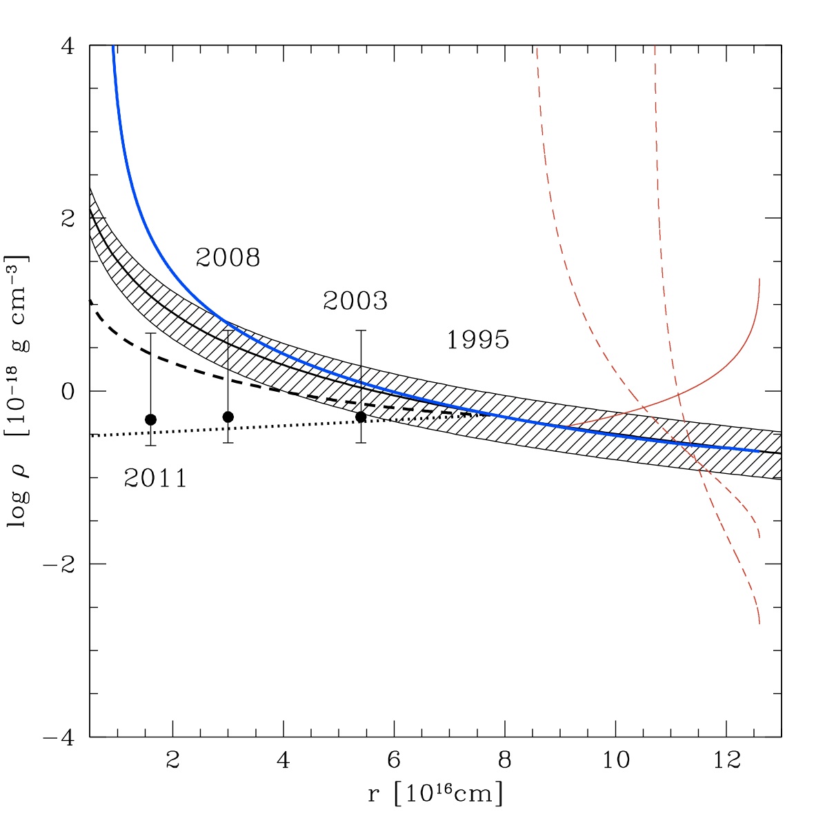
Figure 2: The dashed region shows the expected density of G2 as function of orbital radius r, assuming pressure equilibrium with the surrounding hot bubble. The three labeled data points show lower limits of the observationally inferred cloud density. All lines correspond to the evolution of a cloud in a time varying external gas component with a pressure that increases with time as expected for G2 on its orbit into the center. With the exception of the dotted black line, tidal effects are neglected. The thick dashed line shows the theoretically expected density of G2 if it formed as a spherical cloud in the year 1995, neglecting tidal effects. For comparison, the dotted black line shows the mean density evolution of the numerical simulation CC01, starting also in 1995 (Section 6.1), where tidal effects are included. The thick blue line shows the density evolution if G2 started at apocenter. Dashed red lines correspond to the evolution of a cloud that starts with a pressure that is a factor of 10 or 100 smaller at apocenter than required for pressure equilibrium. The solid red line shows the early expansion phase of an overpressured cloud with initial density that is a factor of 100 larger than the equilibrium density.

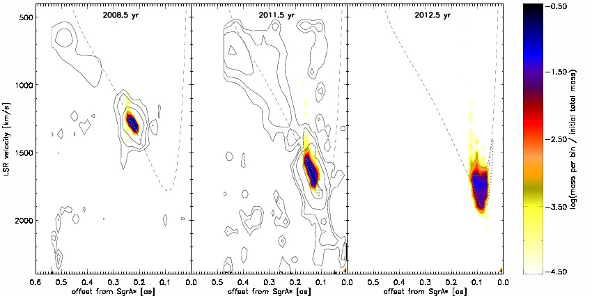
Figure 5: Position versus line-of-sight velocity map of the ”in-situ” formation model CC01 (see also Figure 2 of Gillessen et al. 2012), which corresponds to a cloud that forms in 1995. The contours show the Br$\gamma$ emission of G2, obtained with SINFONI on the VLT (Gillessen et al. 2012). Colors correspond to the total mass of gas as predicted by the simulation in each position-velocity bin with the values given by the color bar. The dashed line shows the ballistic orbit of a point particle in the gravitational potential of the SMBH, centered on G2. The dotted lines show the distribution if each gas element of the cloud would move on a balistic orbit. In 2008.5 the cloud is still compact. Over the next 3 years its develops a strong velocity shear. Overall the calculations are in excellent agreement with the observations. The predicted structure of G2 in the PV-diagram for the year 2012.5 is shown in the right panel.

Strong observational evidence for a cold cloud component in the Galactic center has recently been reported by Gillessen et al. (2012). They detected a dense, dusty and ionized gas clump which we will call G2 (another cloud, G1, has been discovered earlier by Clênet et al. (2005)) with a dust temperature of merely 550 K and a gas temperature of order $10^{4}$ K, representing a relatively cold droplet of ionized gas, embedded in the diffuse $10^{8}$ K gas of the central hot bubble. The cloud’s radius is resolved in the direction of its orbital motion but unresolved in the perpendicular direction. Gillessen et al. (2012) adopt an effective, spherical radius in 2011.3 of 15 mas which corresponds to $1.875\times 10^{15}$ cm. For case B recombination and a mean molecular weight of $\mu=0.6139$ the observed Br$\gamma$ luminosity implies a cloud density of $\rho_{c}\approx 6.1\times 10^{-19}f_{V}^{-1/2}$ g cm^-3 with a corresponding cloud mass of M${}_{c}\approx 1.7\times 10^{28}f_{V}$ g or approximately 3 Earth masses. Here $f_{V}\leq 1$ ist the volume filling factor. In this paper we will investigate scenarios where the cloud is a compact region of cold gas and therefore adopt $f_{V}=1$. The observations (contours in Figure 5; see also Figure 2 in Gillessen et al. 2012) indicate, that G2 might be the upstream compact head of a larger, diffuse distribution of cold gas. The total mass of this system could be substantially larger than G2’s estimated mass.

The cloud is approaching Sgr A^∗. Its orbit could be traced back for the past 10 years, allowing a detailed orbital analysis which shows that G2 is moving on a highly eccentric orbit. In 2013.5 the cloud will pass the SMBH at a pericenter distance of merely 3100 times the event horizon, corresponding to $4.0\pm 0.3\times 10^{15}$ cm. The next two years will therefore provide a unique opportunity to investigate directly the disruption of a cold gas clump by its gravitational interaction with the SMBH and maybe even the onset of a new activity cycle, triggered by the accretion of gas onto the central black hole. In fact, clear evidence for ongoing tidal velocity shearing and stretching has already been detected.

The existence of a tiny, cold gas cloud in the near vicinity of the SMBH, embedded in the hostile $\sim 10^{8}$ K gaseous environment, is surprising and raises numerous interesting questions. Where did this cloud come from and where will it go? Why is it on such a highly eccentric orbit? Which processes constrain the physical properties of G2, i.e. its size, mass, density, temperature and geometrical shape. How many clouds like G2 are currently orbiting Sgr A^∗ and how do they affect its activity and gas accretion rate?

In this paper we will investigate some of these questions, focussing on a simplified prescription of the cloud’s structure and evolution. More detailed numerical simulations will be presented in subsequent papers. Section 2 discusses possible formation scenarios. Section 3 summarizes the orbital properties of G2 which have implications for its formation. Section 4 investigates the various hydrodynamical processes of interaction between G2 and its surrounding that constrain G2’s origin, orbit and evolution. In Section 5 we show that G2 can in turn be used as a sensitive probe to explore the thermodynamics of the diffuse gas component in the Galactic Center. Section 6 finally presents a first set of hydrodynamical simulations that explore the evolution of a cold gas cloud, moving through a hot, stratified medium within the gravitational potential of the SMBH. The results are summarized and conclusions are drawn in Section 7.

2 FORMATION SCENARIOS

Possible formation scenarios can be broadly subdivided into two categories, the diffuse cloud scenario versus the compact source scenario.

2.1 The Diffuse Cloud Scenario

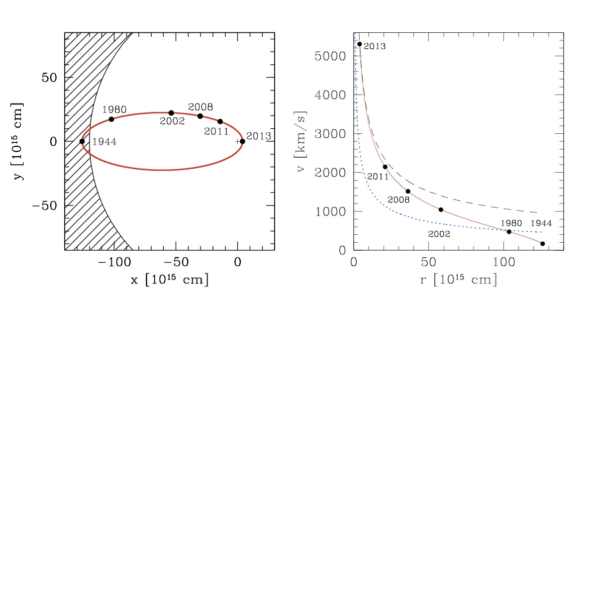
Figure 1: The left panel shows the orbit and location of G2 in the orbital plane. G2’s apocenter coincides with the inner edge of the clockwise rotating stellar disk (shaded area). The cloud will pass the SMBH (cross) in 2013 at a distance of merely $\sim 3100$ times the event horizon. Due to its highly eccentric orbit, the cloud spends most of its time in the outer regions. The right panel shows the velocity of G2 as function of its distance r from the SMBH. For comparison, the dashed line shows a parabolic, unbound orbit with total energy E=0. The dotted line shows the local sound speed of the diffuse, hot environment (Equation 3).

The diffuse cloud model assumes that G2 is a cold gas clump, embedded in and confined by the hot gaseous environment of the central bubble. For the densities and temperatures of the diffuse hot gas in the Galactic Center, the cooling timescale of the hot gas is much longer than the dynamical timescale (Cuadra et al. 2005; Quataert 2004). Cloud formation due to a cooling instability (Field, Goldsmith & Habing 1969; Burkert & Lin 2000) of the hot gas can therefore be ruled out as a formation mechanism. The most likely scenario is probably that G2 originates from the complex two-phase medium in one of the two disks of young massive stars that surround the central bubble. Shocked, fast winds of young massive stars with velocities of order 1000 km/s generate hot $10^{8}$ K plasma, that partly is gravitationally capture by the SMBH and forms the central hot bubble. In contrast, slow winds from luminous blue variable candidates with velocities of 300-500 km/s when shocked are heated only to $10^{6}$ K and subsequently cool fast, leading to the formation of cold, bound cloudlets, embedded in the hot intercloud medium. Interestingly, the orbital plane of G2 coincides with the clockwise disk of young, massive O and Wolf-Rayet stars and its apocenter distance agrees with the disks’s inner edge (left panel of Figure 1). This supports the notion that the cloud might indeed be shocked wind debris. The circular velocities of the stars in the disk are of order 700 km/s while G2 started on a highly eccentric orbit with a tangential velocity at apocenter of order 200 km/s (see Section 3). For typical wind velocities of 500 km/s and assuming a rotational velocity of the star of order 700 km/s, clumps might then have rotational velocities that range between 1200 km/s upstream and 200 km/s downstream. While the upstream clumps might be ejected from the Galactic center, downstream clumps would have just the correct initial velocity to fall into the center on a highly eccentric orbit, like G2. One of the implications of this model is that cold clumps with a large spectrum of masses and orbital parameters should continuously be produced by this process in the stellar disks with many of them falling into the central region on a highly eccentric orbit. We will show however in the subsequent sections that G2’s mass is special in the sense that clumps with masses larger than G2 might easily break up into smaller pieces while smaller clumps evaporate quickly.

2.2 The Compact Source Scenario

Within the framework of the compact source scenario, G2 represents the visible diffuse gas atmosphere of an unresolved, dense object in its center that might continuously loose gas (Gillessen et al. 2012; Murray-Clay & Loeb 2012). The object might have formed $10^{6}$ yr ago in the stellar disk and was scattered into a highly eccentric orbit due to a close encounter with another star or massive black hole. Gillessen et al. (2012) argue that the gas cloud must be optically thin. In order to be invisible its central, compact object has to be either hotter than $10^{4.6}$ K, emitting most of its light in the ultraviolet with a low enough luminosity of $<10^{3.7}$ L_⊙ or very cold. Gillessen et al. suggest a compact planetary nebula as a possible candidate. Murray-Clay & Loeb (2012) propose a dense, protostellar disk, bound to a low-mass star. Another possibility might be an evaporating low-mass star, brown dwarf or Jupiter-like planet.

In order to distinguish between the different scenarios and determine G2’s nature it is important to find constraints that need to be met by any viable model. In the following sections we will investigate characteristic properties of G2’s structure and orbit which are provide information about the properties of the confining hot gaseous environment. We then focus on the diffuse cloud scenario in detail using hydrodynamical simulations that follow the cloud on its way towards pericenter and dispersal afterwards.

3 ORBITAL PARAMETERS OF G2 AND ITS LOCATION OF BIRTH

Measurements of the position and velocity of G2 tightly constrain its orbit (see Gillessen et al. 2012 for details). Adopting a SMBH mass of $4.31\times 10^{6}$ M_⊙ and a Sun - Galactic Center distance of 8.33 kpc, the orbital eccentricity is e=0.9384 $\pm 0.0066$ with a period of 137.8 $\pm 11$ years and a semi-major axis of 6.49 $\pm 0.35\times 10^{16}$ cm. The left panel of Figure 1 shows the orbit of the cloud. For a Keplerian orbit, G2 would have been at apocenter in the year 1944.6, with a distance from the SMBH of r_apo = 1.26 $\pm 0.06\times 10^{17}$ cm. In 2011.5 its distance was 1.8 $\times 10^{16}$ cm. It will reach pericenter in 2013.5 with a distance of merely r_peri = 4.0 $\pm 0.3\times 10^{15}$ cm. Due to its highly eccentric orbit, the cloud spends most of its time at large radii r $\geq 5\times 10^{16}$ cm.

Our simulations (Section 6) show that the cloud will not survive its pericenter passage. If it formed close to its presently observed radius (”in situ” scenario, see Section 6.1), we would be very fortunate to have discovered it before it is disrupted. Although such a coincidence cannot be ruled out, it is more likely that the cloud formed close to apocenter at r $\geq 10^{17}$ cm at the inner edge of the clockwise disk (shaded area in the left panel of Figure 1).

The right panel of Figure 1 shows the velocity of the cloud as function of its distance from the SMBH. If G2 started at apocenter, its velocity was v=168 $\pm$ 80 km/s which is much smaller than its circular velocity of 676 km/s. In 2011.5 its velocity had increased to v=2360 $\pm$ 50 km/s and at pericenter it will have accelerated to a velocity of 5264 $\pm$ 300 km/s. For comparison, the dashed line corresponds to the velocity expected for an object on a parabolic orbit. The cloud is gravitationally bound to the SMBH with a binding energy per mass of

$$E_{b}/M_{c}=\frac{1}{2}v^{2}-\frac{GM_{BH}}{r}=-4.4\times 10^{15}\mathrm{erg/g}.$$ (1)

For a total cloud mass of M${}_{c}=1.7\times 10^{28}f_{V}$g, the total binding energy would then be $E_{b}=-7.5\times 10^{43}f_{V}$ erg.

4 INTERACTION WITH THE HOT SURROUNDING GAS

Up to now we assumed a Keplerian orbit. G2’s motion is however affected by its hydrodynamical interactions with the confining, hot gaseous surrounding (Gillessen et al. 2012). Here, we adopt the Yuan et al. (2003) model (see also Xu et al. 2006) which reproduces the Chandra X-ray observations and is consistent with the low accretion rate inferred by Marrone et al. (2007). For a mean molecular weight $\mu=0.614$ the hot gas density distribution in the surrounding of Sgr A^∗ is

$$\rho_{hot}(r)=\rho_{0}\ \frac{r_{0}}{r}=\eta_{hot}\times 9.5\ 10^{-22}\left(\frac{10^{16}\mathrm{cm}}{r}\right)\mathrm{g\rm cm}^{-3}$$ (2)

where $r_{0}=10^{16}$ cm and $\rho_{0}=\rho(r_{0})$. $\eta_{hot}\leq 1$ takes into account the fact that some fraction of the observed X-ray luminosity might be due to unresolved stellar sources (Sazonov, Sunyaev & Revnivtsev 2011). Given the density distribution, the assumption that the hot gas component is close to hydrostatic equilibrium within the SMBH’s gravitational potential would lead to a temperature distribution

$$T_{hot}(r)=T_{0}\frac{r_{0}}{r}=\mu\frac{GM_{BH}}{2R_{g}r_{0}}\ \frac{r_{0}}{r}=2\times 10^{8}\left(\frac{10^{16}cm}{r}\right)K$$ (3)

with T${}_{0}=$T$(r_{0})$. Note that T₀ is independent of the mass loading, i.e. $\rho_{0}$. Our estimate of T₀ is a factor of 2 smaller than the value adopted by Gillessen et al. (2012), taken from the Xu et al. (2006) model with a temperature of T${}_{0}=3.5\times 10^{8}$ K. It is however more consistent with Yuan et al. (2003, their Figure 2). If the hot gas would actually fall inwards as expected for an accretion flow, then T₀ would be even lower. If the temperature would be as high as adopted by Xu et al. (2006), the pressure force exceeds the gravitational force, resulting in an expansion which is in contradiction with the gas infall scenario. The blue dotted line in the right panel of Figure 1 shows the sound speed of the hot bubble, adopting equation 3. The cloud’s velocity is sonic with respect to the hot gas in the outer regions and becomes slightly supersonic (Mach 1.5) further in. We have assumed hydrostatic pressure equilibrium with the gravitational potential of the SMBH. The situation is certainly much more complex. Rotation, convection, thermal winds, heating and cooling processes, thermal conduction and magnetic fields are likely to affect the detailed structure of the hot bubble surrounding Sgr A^∗ (e.g. Johnson & Quataert 2007; Hawley & Balbus 2002). Given the limited amount of data it is currently difficult to constrain models that include these effects. In order to keep the theory simple and well determined, we therefore restrict ourselves in this paper to the simple atmosphere, as given by the equations 2 and 3. Our results and predictions might serve as a first approximation and a test for subsequent, more sophisticated models.

A detailed investigation of the cloud’s evolution and hydrodynamical interaction with the surrounding requires an estimate of its radius R_c and density $\rho_{c}$. In this paper we will follow Gillessen et al. (2012) and assume that the cloud is ionized by the strong UV field of the central cluster of massive stars. Its cooling timescale is (Sutherland & Dopita 1993; Burkert & Lin 2000) $\tau_{cool}=3k_{B}T_{c}/\Lambda n_{c}$ which for a cooling rate of $\Lambda\approx 3\times 10^{-22}$ erg cm³ s^-1 and for cloud densities of n${}_{c}\geq 10^{5}$ cm^-3 leads to $\tau_{cool}\leq 10^{5}$ sec which is much shorter than the orbital period. G2 should therefore maintain its temperature of $T_{c}=10^{4}$ K during most of its evolution, set by photo ionisation equilibrium. Because of its small mass density with respect to its Roche density, self-gravity is completely negligible. In this case, it will try to achieve a homogeneous density state, in pressure equilibrium with the surrounding. The hydrodynamical simulations, presented in Section 6 actually show a more complex structure due to the compression of the front edge by ram pressure while at the same time the back, downstream tail is at slightly lower densities due to tidal shearing. This does however not affect much the cloud’s effective size which, for most of its orbit, is well reproduced by adopting a mean density that is consistent with the assumption of pressure equilibrium: $\rho_{c}=\rho_{hot}T_{hot}/T_{c}$.

Unfortunately, the observations do not resolve G2’s minor axis, perpendicular to the orbital motion. They only provide an upper limit of 12 mas, corresponding to $R_{c}\leq 1.5\times 10^{15}$ cm. The 2008.3 position versus line-of-sight velocity (PV) diagram (left panel of Figure 5) shows a velocity gradient that can be used in order to determine the elongation of the cloud along its orbit which in this stage corresponds to a major axis radius of 21 mas or $2.6\times 10^{15}$ cm and a minor axis of $\leq 1.5\times 10^{15}$ cm. Adopting a cylindrical shape as expected for a tidally elongated object, a lower limit of its density in 2008 is then $\rho_{c}\geq 5\times 10^{-19}$ g cm^-3. The cloud has been in this compact state from the earliest spectral measurements that date back to 2002 till 2008. In 2011.5 (middle panel of Figure 5) the cloud has developed a much stronger velocity shear due to the gravitational acceleration. Its corresponding major-axis length is 22 mas or 2.75$\times 10^{15}$cm, leading to a cloud density that has not changed much till 2008 if one adopts a constant minor axis radius. As the minor-axis is not resolved, the cloud’s density in 2011 could however be substantially larger than in 2008 as it might have been stretched and compressed into a dense, thin, spaghetti-like filament (see Section 6).

Several non-linear and complex hydrodynamical processes dominate G2’s interaction with its surrounding, diffuse gas. These include evaporation, ram pressure, gas stripping, cloud compression or expansion as well as Rayleigh-Taylor and Kelvin-Helmholtz instabilities. In addition, the cloud might be affected by compressional heating and cooling and might be threaded by magnetic fields. A detailed investigation of all these simultaneously acting processes requires self-consistent numerical simulations which are beyond the scope of this paper. Here we restrict ourselves to some of the most basic aspects, leaving more detailed models to subsequent papers. We start with a discussion of the most dominant processes in isolation and then present a first set of numerical simulations that investigate especially the tidal effects onto G2’s evolution.

4.1 Cloud Evaporation

Small gas clouds, embedded in a hot environment, will loose gas due to evaporation as a result of thermal conduction. The classical thermal conductivity (Spitzer 1962; Parker 1963) is based on the diffusion approximation which assumes that the electron mean free path $\lambda_{e}$ of the hot medium is small compared to the cloud radius $R_{c}$. Cowie & McKee (1977) in their seminal paper demonstrate that this approximation is invalid as soon as $\lambda_{e}\geq R_{c}$ that is if the saturation parameter $\sigma_{0}=1.84\ \lambda_{e}/R_{c}>1$ . In this case, the heat flux is no longer determined by the classical diffusion formula.

For the central hot bubble we find

$$\lambda_{e}=10^{4}\left(\frac{T}{\mathrm{K}}\right)^{2}\left(\frac{10^{-21}\mathrm{gcm}^{-3}}{\rho_{hot}}\right)\mathrm{cm}=4\times 10^{17}\left(\frac{10^{16}\mathrm{cm}}{r}\right)\mathrm{cm}$$ (4)

which for all relevant distances r from the SMBH is indeed much larger than G2’s observed size $R_{c}$. Adopting a typical cloud radius of order $1-2\times 10^{15}$ cm the corresponding saturation parameter is $\sigma_{0}\approx 50-500$. In the saturated limit and assuming pressure equilibrium between the cloud and the hot surrounding, the evaporation timescale is given by (Cowie & McKee 1977)

$$\tau_{evap}=120yr\left(\frac{r}{10^{16}\mathrm{cm}}\right)^{1/6}\left(\frac{M_{c}}{1.7\times 10^{28}\mathrm{g}}\right)^{1/3}.$$ (5)

Cowie & McKee (1977) argue that for a wide variety of conditions, the presence of a magnetic field does not strongly affect this timescale. Interestingly, this evaporation timescale is very similar to the orbital period of 138 yr. Equation 5 provides a strong lower limit on the mass of cold dust clouds that can penetrate as deeply into the hot bubble as observed for G2. Only clouds with masses of order or larger than G2 would reach distances of 1-2 $\times 10^{16}$ cm. We also can conclude that, once G2 breaks up at pericenter, its subfragments might dissolve quickly. Note however that the mixing of cloud material with the diffuse surrounding will change the thermodynamical properties of the bubble. According to equation 2 the total mass of hot gas in the inner $2\times 10^{16}$ cm is similar to G2’s mass. Mixing of cloud debris with the environment could effectively cool the innermost region of the hot bubble which would reduce the efficiency of evaporation. In addition, this process might destabilize the atmosphere which then collapses onto the SMBH. The situation is different in the outer orbital parts where the mass of the hot bubble is more than a factor of 100 larger that G2’s mass.

4.2 Ram pressure effects

Ram pressure will compress the cloud into a lenticular and sickle-shaped structure (e.g. Murray & Lin 2004; Schartmann, Krause & Burkert 2011). The importance of ram pressure, compared to the thermal pressure of the surrounding is given by the ratio v²/c${}_{hot}^{2}$, where c_hot is the sound speed of the hot gas component. As shown by the blue dashed line in the right panel of Figure 1, close to apocenter, gas pressure dominates while at its present location ram pressure is a factor of 2-3 larger than the thermal pressure.

The drag will also remove part of the cloud’s orbital energy. Given the highly eccentric orbit, we can to a good approximation neglect the cloud’s small tangential motion. In this case, the energy lossed by G2 on its way from radius $r_{1}$ to radius $r_{2}$ is (Murray & Lin 2004)

$$\Delta E_{drag}=\frac{1}{2}\pi C_{D}\int_{r_{1}}^{r_{2}}R_{c}^{2}\rho_{hot}(r)v^{2}(r)dr.$$ (6)

where $C_{D}\approx 1$ is the drag force. The observations already demonstrate that, within the observational errors, G2 follows a Keplerian orbit. $\Delta E_{ram}$ therefore should be small, compared to the cloud’s kinetic and absolute potential energy. In this case we can use $v(r)$ from equation 1 and assume $E_{b}/M_{c}$ to be roughly constant. For a constant cloud radius $R_{c}$ the integration of equation 6 leads to

$$\Delta E_{ram}(r)=\pi\rho_{0}r_{0}C_{D}R_{c}^{2}\left[\frac{E_{b}}{M_{c}}\ln\left(\frac{r_{2}}{r_{1}}\right)-GM_{BH}\left(\frac{1}{r_{2}}-\frac{1}{r_{1}}\right)\right].$$ (7)

Adopting $C_{D}=1$ and an effective cloud radius of $R_{c}=2\times 10^{15}$ cm, the energy lossed between apocenter and $r_{2011.5}=1.8\times 10^{16}$cm due to ram pressure effects would be $\Delta E_{ram}(r_{2011.5})=2\eta_{hot}\times 10^{42}$erg = $0.03\eta_{hot}E_{b}$. This confirms that the cloud moves on a ballistic orbit during its approach of the SMBH. It also indicates that our estimate of G2’s apocenter is robust. For such an extended cloud, ram pressure effects would however change the cloud’s orbit substantially within the next 2 years on its way towards pericenter with $\Delta E_{ram}(r_{peri})=2\eta_{hot}\times 10^{43}$ erg = 0.3 $\eta_{hot}E_{b}$. It is unlikely to assume a fixed size as the cloud will continuously try to achieve pressure equilibrium with its surrounding. If $\rho_{c}=\rho_{hot}T_{hot}/T_{c}$ and adopting a spherical geometry the energy loss is

$$\Delta E_{ram}(r)=\pi\eta_{hot}^{1/3}\left(\frac{\rho_{0}}{r_{0}}\right)^{1/3}\left(\frac{3M_{c}T_{c}}{4\pi T_{0}}\right)^{2/3}\left[\frac{3}{4}\frac{E_{b}}{M_{c}}\left(r_{2}^{4/3}-r_{1}^{4/3}\right)+3GM_{BH}\left(r_{2}^{1/3}-r_{1}^{1/3}\right)\right].$$ (8)

Now, for $T_{c}=10^{4}$ K, on its way from apocenter to $r_{2011.5}$, the cloud would loose $\Delta E_{ram}(2011.5)=0.02\eta_{hot}^{1/3}E_{b}$. This value increases to 0.04 $\eta_{hot}^{1/3}$ till pericenter which is much smaller than the constant radius case due to the strong compression of the cloud at small orbital radii. To a good approximation, the cloud should then stay on a Keplerian orbit till pericenter.

4.3 Pressure Confinement, Implosion and Hydrodynamical Instabilities

As self-gravity is negligible, for a constant temperature $T_{c}$, the cloud will try to achieve a homogeneous density state, in thermal pressure equilibrium with the surrounding. The shaded region in Figure 2 indicates the expected cloud density $\rho_{equi}$ for the case of pressure equilibrium with the surrounding. The thick black line shows $\rho_{equi}$, adopting a hot gas temperature and density as given by the equations 2 and 3, with $T_{c}=10^{4}$ K. The lower and upper boundaries correspond to $\eta_{hot}=0.5$ and $T_{0}=2\times 10^{8}$ K and $\eta_{hot}=1$, $T_{0}=3.5\times 10^{8}$ K, respectively. Labeled black points show G2’s estimated density assuming its minor axis is marginally resolved. In this case, the cloud would have been in pressure equilibrium in 2003. $\rho_{equi}$ increases strongly between 2003 and 2011. In contrast, the observations reveal an increasing velocity gradient in the cloud as expected with decreasing orbital radius. Interestingly, the change in the velocity gradient is consistent with the assumption that G2’s major axis remains roughly constant. The assumption of a minor axis close to the resolution limit then leads to a constant cloud density after 2003 that does not change significantly with time. The cloud’s thickness in the unresolved direction perpendicular to its motion might however decrease continuously. In this case $\rho_{c}$ would increase with time. The 2008 and 2011 points in Figure 2 then represent lower limits.

We unfortunately do not have detailed information about the cloud’s structure prior to 2003. One can however investigate the question whether a cloud like G2 could have achieved pressure equilibrium in 2003 if it started with an arbitrary density at apocenter. The implosion of a gas clump that is imposed to a high pressure environment has been studied in details by Klein, McKee & Colella (1994). A shock front forms at the outer edge that sweeps up the cloud. It accelerates till the sum of the ram-pressure of the shock $\rho_{c}v_{s}^{2}$ and the internal gas pressure $P_{c}=\rho_{c}c_{c}^{2}$ with c_c the cloud’s internal sound speed is equal to the external pressure $P_{hot}=\rho_{hot}c_{hot}^{2}$, with c_hot the local sound speed of the surrounding gas, leading to an equilibrium shock velocity of

$$v_{s}^{2}=\left(\frac{\rho_{hot}}{\rho_{c}}\right)c_{hot}^{2}-c_{c}^{2}.$$ (9)

The cloud’s crushing timescale is then

$$\tau_{cc}=\frac{R_{c}}{v_{s}}=0.5\tau_{s}\left(\frac{P_{hot}}{P_{c}}-1\right)^{-1/2}$$ (10)

where $\tau_{s}=2R_{c}/c_{c}$ is the cloud’s sound crossing timescale which for our typical parameters of a $10^{4}$ K gas clump, in an environment, described by the equations 2 and 3 leads to

$$\tau_{s}=2\left(\frac{3M_{c}}{4\pi c_{c}P_{c}}\right)^{1/3}=176\ \eta_{hot}^{-1/3}\left(\frac{r}{r_{apo}}\right)^{2/3}\left(\frac{P_{hot}}{P_{c}}\right)^{1/3}yr.$$ (11)

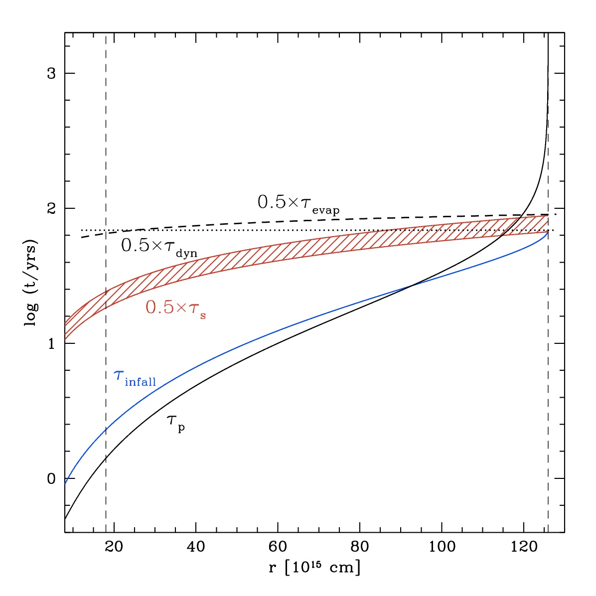
Figure 3: The various timescales are shown as function of distance r from the SMBH that affect G2’s evolution: the dynamical timescale $\tau_{dyn}$ (black, horizontal dotted line), the evaporation timescale $\tau_{evap}$ (black dashed line), the sound crossing timescale $\tau_{s}$ (shaded red region), adopting $\eta_{hot}=1$ (upper limit) and $\eta_{hot}=0.75$ (lower limit), respectively, the pressure timescale $\tau_{p}$ (black solid line) and the infall timescale $\tau_{infall}$ (blue solid line) that measures the time it takes G2 to reach pericenter from radius r. The two vertical dashed lines correspond to the apocenter and the location of G2 in 2011.3, respectively.

Figure 3 shows G2’s sound crossing timescale (red shaded region) as function of orbital radius, assuming pressure equilibrium $P_{hot}=P_{c}$. Interestingly, close to apocenter, $\tau_{s}$ is almost equal to the dynamical time (orbital period) shown by the horizontal dotted line.

Equation 10 demonstrates that for $P_{hot}>>P_{c}$ the crushing timescale of the cloud is much smaller than its sound crossing time and dynamical timescale. Starting close to apocenter, it should therefore implode long before reaching its current position. The dashed, red lines in Figure 2 show the evolution of the mean density of such a cloud. For that, we integrated the evolution of the compression front, taking into account the time variation of $P_{hot}(r)$ as the cloud moves through the stratified environment with the pressure increasing with decreasing distance r(t) from the SMBH. Assuming a constant cloud temperature, the evolution of the outer cloud radius is then given by $dR_{c}/dt=-v_{s}(t)$ where $v_{s}(t)$ depends on the orbital radius r(t) according to equation 9. Note that these clouds, when crossing the shaded area of pressure equilibrium, continue to contract. Clouds that are in pressure equilibrium are one-component systems with a constant gas density. In contrast, the imploding clouds, despite the fact that their volume averaged density is the same, contain an inner, low-pressure and low-density core that is being swept up by a high-density, inwards moving shell.

As the high-density shock front is accelerated by a low-density gaseous environment the cloud will be shredded by Rayleigh-Taylor instabilities that grow on a timescale of (Klein, McKee & Colella 1994)

$$\tau_{RT}=\frac{\tau_{cc}}{(kR_{c})^{1/2}}$$ (12)

The shortest wavelength or largest wave number $k$ has the fastest growth rate. But Rayleigh- Taylor perturbations saturate in the non-linear regime. As a result, the most destructive wavelength is given by $kR_{c}\approx 1$. The cloud should therefore be destroyed and mix with the surrounding on a timescale of order its crushing timescale. In summary, under-pressured clouds, starting at apocenter, would disappear before reaching the presently observed position. If G2 came from apocenter, it therefore was either in pressure equilibrium with the surrounding or had an even larger pressure.

Even if G2 is initially in pressure equilibrium, the pressure of the surrounding hot gas increases fast on its way towards the SMBH. The cloud will be able to adjust as long as $\tau_{s}$ is short compared to the timescale $\tau_{p}$ on which the external pressure changes

$$\tau_{p}=\frac{1}{v_{r}d\ln P_{hot}/dr}=\frac{r}{2v_{r}}$$ (13)

with v_r the radial velocity of the cloud. The solid black line in Figure 3 shows $\tau_{p}(r)$ which for G2’s orbit becomes smaller than $\tau_{s}$ quickly for r $\leq 10^{17}$ cm. Entering this region, the cloud will become a cold, low-pressure island within a high-pressure surrounding and start imploding. The evolution of such a system is shown by the thick, blue line in Figure 2 where we have assumed that the implosion starts as soon as $\tau_{p}<\tau_{s}$. In 2003, G2’s mean density should still be close to $\rho_{equi}$. At that point in the evolution however, the timescale for the shock to completely crunch the cloud has become smaller than the local infall timescale $\tau_{infall}$ and its density now increases fast. Here we have neglected tidal shearing. As we will show in Section 6 tidal effects actually reverse the evolution, leading to a decreasing density when the cloud approaches the inner regions of its orbit.

Within the framework of the ”in situ” scenario, discussed in Chapter 2, the cloud might have formed half-way between apocenter and the SMBH, e.g. in the year 1995, shortly before G2 was detected. The thick, black dashed line in Figure 2 shows the clump implosion for this case. Due to G2’s relatively high initial density, the velocity v_s of the inwards moving shock is now less fast and will not compress the cloud significantly within the next 12 years while the pressure in the surrounding rises steeply. The cloud therefore evolves isochorically, in good agreement with the observations.

G2 might have started at apocenter in a high-density state with a pressure that was larger than in the surrounding gas. In this case, the cloud will first expand with a velocity that should be roughly equal to its sound velocity, trying to achieve pressure equilibrium with the environment. This expansion phase is shown by the solid red line in Figure 2. The subsequent evolution is complex and requires numerical simulations that will be discussed in Section 6.

5 Probing the Temperature and Density Structure of the Central Hot Bubble

G2 is a sensitive probe of the conditions in the central hot bubble. Especially the early observations around 2002-2004, when the cloud is at a distance of $r\approx 5.5\times 10^{16}$ cm provide important constraints on the density and pressure of the surrounding diffuse gas. In the following we will adopt the radial dependence of $\rho_{hot}$ and T_hot as given by the equations 2 and 3. In addition, we assume that the cloud is in pressure equilibrium with its surrounding in these early phases. As discussed in Section 4, a lower limit of the density of G2 in 2002-2008 is $\rho_{c}=5\times 10^{-19}$ g cm^-3. For a cloud temperature of T${}_{c}=10^{4}$ K this implies $\rho_{hot,2002}T_{hot,2002}=0.033\times\rho_{0}T_{0}\geq 5\times 10^{-15}$ K  g/cm³ or

$$\rho_{0}\times T_{0}\geq 1.5\times 10^{-13}\mathrm{gcm^{-3}K}.$$ (14)

If $\rho_{0}\leq\eta_{hot}\times 10^{-21}$ g cm^-3, as inferred from the Chandra observations (Xu et al. 2006), $T_{0}\geq 1.5\times 10^{8}/\eta_{hot}$ K which is in agreement with Equation 3 if $\eta_{hot}=0.75$. This would indicate that the fraction $\eta_{hot}$ of X-ray luminosity, resulting from unresolved stellar sources (Sazonov, Sunyaev & Revnivtsev 2011), is small as $T_{0}$ cannot be much larger than a few $2\times 10^{8}$ K if the hot bubble is bound to the SMBH.

6 Hydrodynamical Simulations

In order to validate the results obtained from our analytical estimates and to investigate the future evolution of the cloud we have conducted idealised hydrodynamical simulations.

The hydrodynamical equations were integrated with the help of PLUTO, version 3.1.1 (Mignone et al. 2007) which is a fully MPI-parallelized, high resolution shock capturing scheme with a large variety of Riemann-solvers. For all simulations shown in this article, we propagated the state vector with the two-shock Riemann solver, did a parabolic interpolation and employed the third order Runge-Kutta time integration scheme. In these first simulations, we were interested in the evolution of the cloud in an idealised atmosphere with a smooth density and pressure distribution in concordance with observations, as discussed in Section 4. In order not to be dominated by the interaction of the cloud with disturbances of the convectively unstable atmosphere, we artificially stabilise it. This was done by additionally evolving a passive tracer field ($0\leq tr\leq 1$), which allowed us to distinguish between those parts of the atmosphere which have interacted with the cloud ($tr\geq 10^{-4}$) from those which changed due to the atmosphere’s inherent instability ($tr\leq 10^{-4}$). Those cells fulfilling the latter criterion were reset to the values expected in hydrostatic equilibrium. The boundary conditions were set to the values expected for hydrostatic equilibrium, enabling outflow but no inflow. The adiabatic index $\Gamma$ was set to one, which we consider a reasonable assumption, as the temperature structure of the advection-dominated accretion flow solutions (e.g. Narayan & Yi 1994; Narayan 2002) is supposed to be given by adiabatic heating of the accretion flow itself and the temperature of the cloud material is expected to be set by photoionisation equilibrium in the radiation field of the surrounding stars (Gillessen et al. 2012). Our two-dimensional computational domain represents the orbital plane of the cloud, which initially starts in pressure equilibrium with the atmosphere except for simulation CC03, initially having an overpressure of a factor of 100. The corresponding parameters are summarised in Table 1. The cloud starts on the negative x-axis of the fixed cartesian coordinate system with a spatial resolution of $7\times 10^{13}$cm ranging from $-1.3\times 10^{17}$cm to $1.2\times 10^{16}$cm in x-direction and $-6.2\times 10^{16}$cm to $2.5\times 10^{16}$cm in y-direction. It orbits in clockwise direction with the major axis parallel to the x-axis and the pericenter of the orbit on the positive x-axis. The black hole is located at the origin of our coordinate system. We neglect magnetic fields as well as feedback from the central source for the sake of simplicity and will give a more detailed analysis of the simulations and numerical tests of this approach in Schartmann et al. (2012).

6.1 Model CC01: In Situ Formation of G2

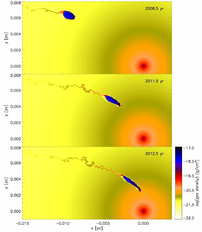
Figure 4: Early phases of the evolution of a cold gas cloud (model CC01) with a mass equal to G2 that starts in pressure equilibrium with the surrounding as a spherical clump in the year 1995. Colors correspond to the logarithm of gas density. White dotted contours correspond to a test particle simulation where gas particles move on ballistic orbits.

Figure 4 shows the evolution of a cloud that was born as a spherical droplet in the year 1995 at a distance of 7.6 $\times 10^{16}$ cm. Dotted white contours depict the expected shape of the cloud from a collisionless test particle simulation, if each gas particle would move on a ballistic orbit within the gravitational potential of the SMBH. In 2008.5 the hydrodynamical interaction with the surrounding is still small and the cloud’s structure follows the outer contour of the test particle simulations very well. The cloud already in this early phase is developing an elongated structure due to tidal effects. Ram pressure stripping at the outer edge also generates a trailing tail of gas that is dispersed by Kelvin-Helmholtz instabilities. The mass loss is however negligible. In 2011.5 and 2012.5 the cloud has become significantly more elongated. Ram pressure effects are now more clearly visible at the front side which is falling behind the ballistic orbits. The dotted black line in Figure 2 shows the mean density evolution as function of orbital radius. In agreement with our analytical estimates (dashed black line in Figure 2), the cloud’s density is not changing significantly between 1995 and 2011 as the crushing timescale for an object that starts in 1995 is longer than its infall timescale. While the mean density in the idealized model is continuously rising due to compression, it actually decreases slowly in the numerical simulation due to the tidal shearing along the orbit. This might be partly an artifact of the 2-dimensional simulations and needs to be confirmed by future 3-dimensional models.

Figure 5 compares the structure of the simulated cloud in the PV-diagram with the observations. In the year 2008.5 the cloud is still compact. In 2011.5 it has developed a strong shear that follows the center-of-mass, ballistic orbit (dashed line). Overall the structure of the simulated cloud in the PV-diagram is in excellent agreement with the observations (contours). The predicted structure and kinematics in 2012.5 is shown in the 3rd panels of the Figures 4 and 5 when the cloud has reached the point of maximum line-of-sight velocity. In the PV-diagram the cloud’s contours still do not deviate significantly from a ballistic orbit, shown by the dotted lines.

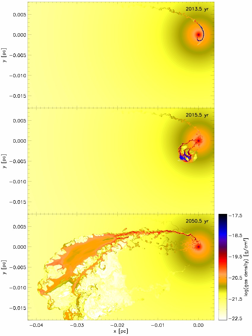
Figure 6: Late phases of the evolution of model CC01. In the year 2050 the cloud has broken up into a long filament that feeds Sgr A^∗.

Figure 6 shows G2’s structure for the ”in situ” scenario during and after pericenter passage. At pericenter the cloud will be tidally stretched into a long, curved filament. As discussed in Section 4.2 the hydrodynamical drag is not strong enough to remove a large fraction of the cloud’s kinetic energy. As a result, the bulk of the gas is moving out to large distances again. Ram pressure at the head has however removed a substantial amount of kinetic energy and angular momentum forcing the front of the filament to fall into the unresolved inner accretion zone of Sgr A^∗ (upper panel). The middle panel of Figure 6 shows that on its way outwards the gas is first compressed both by the negative divergence of the velocity field and by ram pressure. Large Kelvin-Helmholtz eddies are now visible at the inner edge, facing the SMBH, that begin to destroy the cloud, leading to several narrow gas streams that fall into Sgr A^∗. In 2050.5 the cloud has completely dissolved and generated a narrow, dense stream of cold gas that feeds the SMBH.

6.2 Model CC02: Formation of G2 at Apocenter

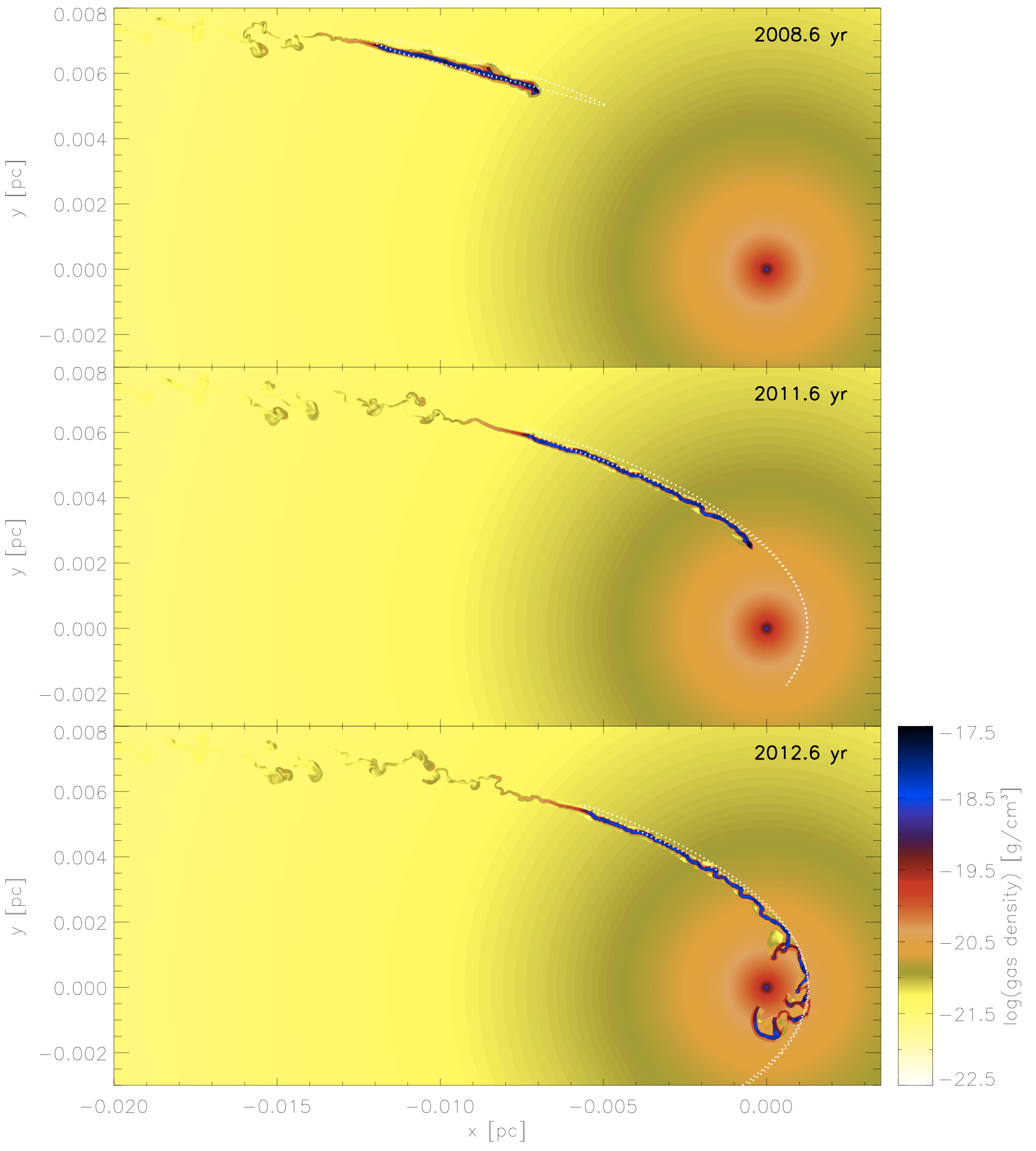
Figure 7: Same as Figure 4 for model CC02. Now the cloud starts in pressure equilibrium at apocenter.

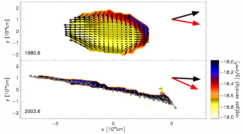
Figure 8: Density distribution and velocity field in the cloud in model CC02 that starts in pressure equilibrium at apocenter. The upper panel shows the early cloud structure in the year 1980.6. The two large vectors show the radial direction towards the SMBH (red) and the mean orbital velocity vector (black) of the cloud, respectively. The velocity field represents the internal velocity of the cloud’s gas after subtracting the center-of-mass velocity (large black arrow). The size of the velocity vectors scale linearly with velocity. As reference, the large arrows in the upper and lower panel correspond to a velocity of 485 km/s and 1135 km/s, respectively. The cloud is compressed perpendicular to its orbit and tidally sheared along its orbit. Due to ram pressure a high-density shell is visible at the upstream front of the cloud. The lower panel shows the structure in the year 2003.6. The cloud has been torn apart into a long spaghetti-like filament.

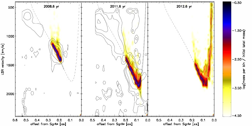
Figure 9: Position-velocity diagram of model CC02, a cloud that starts at apocenter.

We have argued in the Sections 2 and 3 that it is more likely for the cloud to have started in the clockwise rotating stellar disk which agrees with the cloud’s orbital plane and which has an inner edge equal to its apocenter. Figure 7 shows the evolution of an initially spherical, cold gas droplet in pressure equilibrium at apocenter. Initially the cloud remains in pressure equilibrium with its surrounding, in agreement with the analytical estimate (blue line in Figure 2). However even in the early phases tidal effects begin to reshape the cloud. The upper panel of Figure 8 shows the characteristic velocity field in the cloud at 1980.6 after subtracting its center-of-mass motion (large black arrow). The mean cloud density is $2\times 10^{-19}$ g cm^-3, in agreement with our analytical estimates. However, despite the fact that the cloud is still at a distance of $10^{17}$ cm, the strong tidal shear has already generated a strong internal velocity field that pushes material outwards along the orbit while at the same time compressing the cloud perpendicular to it. The surrounding gas pressure, even in combination with the ram pressure is not strong enough in order to stop this flow. Note also that the cloud has developed a density gradient due to ram pressure compression at the front. The lower panel of Figure 8 shows the cloud at 2003.6 when it is at a distance of $5.3\times 10^{16}$ cm. Its mean density has increased to $\rho_{c}=10^{-18}$ g cm^-3 which is in agreement with the observationally inferred cloud density (Figure 2). It is however in disagreement with our analytical estimates that predict higher compression if tidal effects are neglected. This is due to the fact that at this stage tides have turned the cloud into a long filament. The situation has become even more extreme in 2011.6 (middle panel of Figure 7) where the filament has grown to a length of $3\times 10^{16}$ cm which is much longer than the observationally inferred length of $\leq 3\times 10^{15}$ cm. Note that the filament is distorted by Kelvin-Helmholz instabilities as a result of its interaction with the diffuse surrounding. In 2012.6 (lower panel of Figure 7), these instabilites have become non-linear and begin to break up the system into a string of clumps that begin to fall into the SMBH. The PV-diagramm shown in Figure 9 confirms that the structure is much too elongated compared to the observations.

6.3 Model CC03: An Overpressured High-Density Cloud at Apocenter

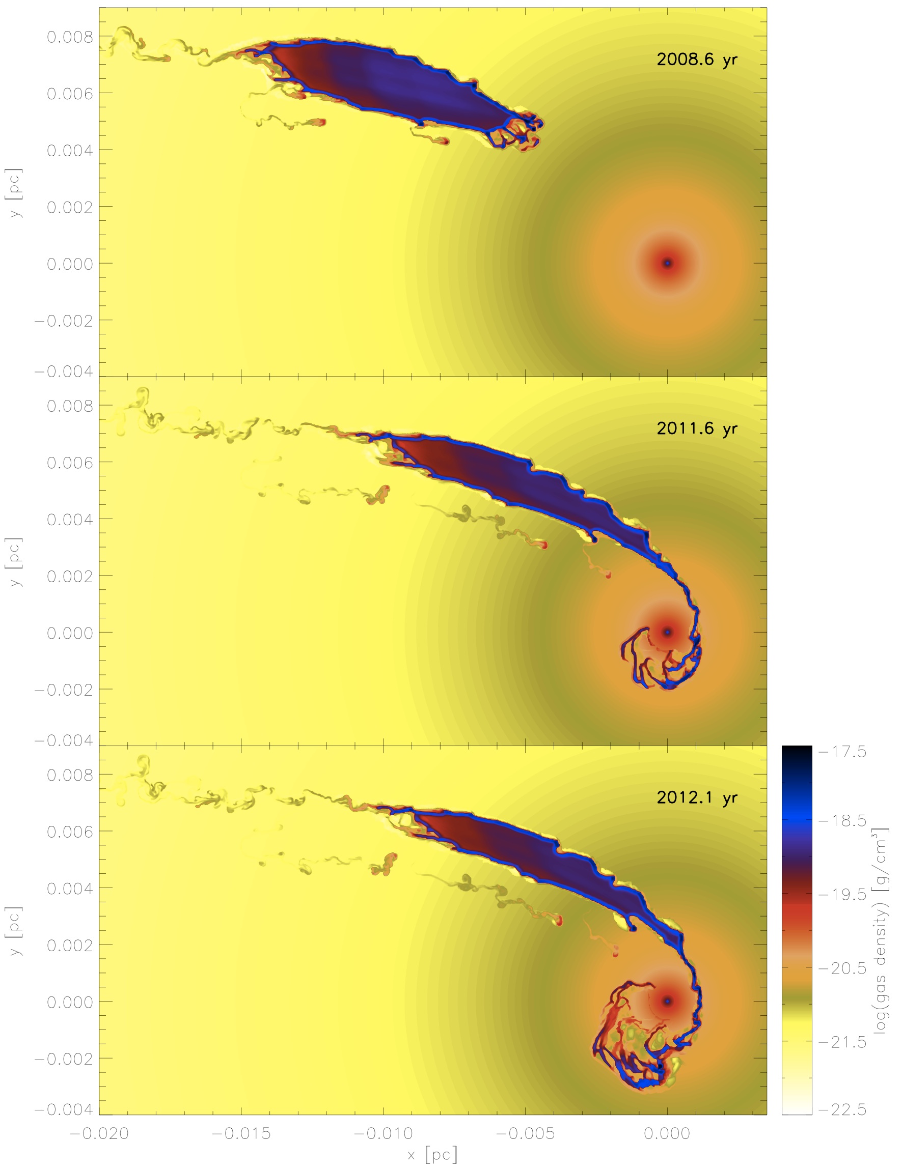
Figure 10: Evolution of model CC03, a cloud that starts at apocenter with a density and pressure that is a factor of 100 larger than its surrounding. Due to the resulting expansion the cloud evolves into a large clump with an internal pressure that is significantly smaller than the surrounding.

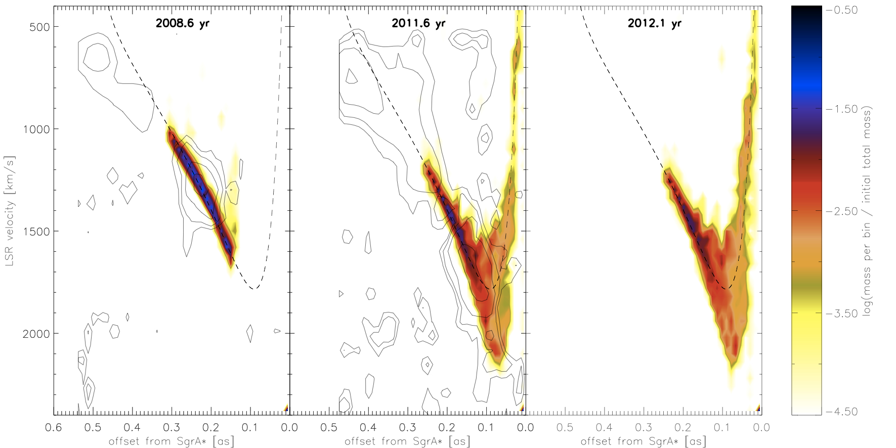
Figure 11: PV-diagram of model CC03.

We argued in the analytical part (Section 4) that a cloud that has a pressure much larger than its surrounding will expand. The detailed evolution is however difficult to predict analytically. We therefore show in Figure 10 the evolution of a clump that started at apocenter with an initial density that is a factor of 100 larger than the equilibrium density $\rho_{equi}$. The cloud initially expands, but the expansion does not stop as soon as the mean cloud density has become equal to $\rho_{equi}$ due to the outwards directed velocity field. The cloud overshoots this equilibrium point and its density and pressure drop further with the cloud forming a very extended structure that is now subject to the strong tidal forces as shown in Figure 10. Like in the previous case, the PV diagramm (Figure 11) is not at all in agreement with the observations. This confirms our previous conclusion that, if G2 is a diffuse cloud, it started its journey into the center close to pressure equilibrium with the surrounding.

6.4 Model SS01: The Spherical Shell Model

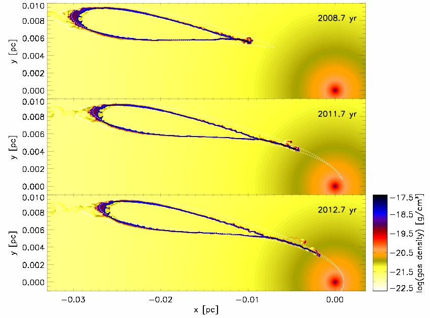
Figure 12: Evolution of the spherical shell model SS01, which assumes that gas is initially distributed in a ring-like structure at apocenter.

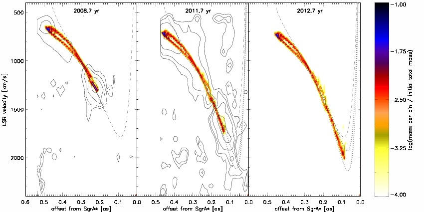
Figure 13: PV-diagram of model SS01 which forms two bright regions of emission with diffuse material in between, similar to the observations.

Up to now we assumed that G2 is an isolated, small few Earth mass cloud that formed either close to the location of first detection or at apocenter. It might however be part of a larger structure. The observations (Figure 2 of Gillessen et al. 2012; contours in the PV diagrams, e.g. Figure 5) indeed show extended emission downstream of G2 with a brighter area at the end that is offset with respect to G2’s orbit with a line-of-sight velocity difference of order 500 km/s. We have tried to generate an initial condition at apocenter that could reproduce these observations and found that a surprisingly simple symmetric shell of gas in the orbital plane with a tangential velocity of 125 km/s, similar to G2’s initial velocity, an outer radius of $1.2\times 10^{16}$ cm and a thickness of $3\times 10^{15}$ cm can reproduce the observations well (table 1). Its gas density $\rho_{c}=1.42\times 10^{-19}$ g cm^-3 is given by the requirement that it is in pressure equilibrium with its surrounding. Such a structure could have been produced either by the dusty wind shells of massive stars, an explosion or an object that crossed the plane of the stellar disk at apocenter. Figure 12 shows the evolution of the shell. G2 in this case represents its leading head that is being compressed into a spheroidal clump as a result of the converging, radial inflow. Interestingly, the projection of this distorted shell along the line of sight also generates a second high surface density region that is connected to G2 by low surface density gas. This is clearly shown in the shell’s PV diagram (Figure 13). Note that this second bright point is also offset with respect to G2’s orbit (dashed line) by $\sim$ 500 km/s, as observed.

7 DISCUSSION AND CONCLUSIONS

We investigated the origin and evolution of the small gas cloud G2 that has been detected approaching the Galactic SMBH on a highly eccentric orbit. The cloud has an observationally inferred density and temperature that during the first years of detection around 2003 indicates that it was in pressure equilibrium with its surrounding. Our analytical estimates and numerical simulations show that it must have formed close to pressure equilibrium. A cloud with a significant lower pressure would be destroyed by implosion while a highly overpressured cloud would go through a phase of rapid expansion, forming a diffuse, extended and tidally elongated structure that is not in agreement with the observations. The ”in situ” cloud scenario which assumes that the cloud formed as a spheroidal clump in pressure equilibrium in the year 1995, shortly before it was detected, provides an excellent match to all the observations, dating back to 2002 till today. In this case, our numerical simulations indicate that the cloud will be tidally stretched into a very elongated filament till 2013.5 which shortly after pericenter passage will begin to loose gas as a result of Kelvin-Helmholtz instabilities. This gas might fall into the inner accretion zone of Sgr A^∗, forming a hot luminous accretion disk. Over the next 80 years the debris of the tidally destroyed cloud will fuel the SMBH, maybe leading to an extended period of nuclear activity.

The main caveat of the ”in situ” model is the fact that we have not been able to identify any physical mechanism that could have formed G2 in 1995. We did not find any known star that was close to its birth place at that time. In addition, the cloud could also not have formed by a cooling instability of the hot gas as its cooling timescale is much longer than the dynamical timescale (Burkert & Lin 2000).

It is intriguing that the assumption of G2 having formed at apocenter leads to several interesting correlations that should be reproduced by any theoretical model of its formation. G2’s orbital plane coincides with the plane of the clockwise rotating stellar disk and its apocenter agrees with the inner disk edge. In addition, G2’s sound crossing timescale, evaporation timescale and orbital timescale are all equal at apocenter. If this is not a coincidence it provides several important constraints on its formation. First of all, G2 obviously did not form very recently (e.g. 1995) by some condensation processes but came from apocenter. It also means that G2 has been in pressure equilibrium at apocenter, either as a result of its formation or due to re-adjustment. It is reasonable to assume that a cloud that is subject to distortions when interacting with a turbulent environment can only maintain coherence if it can react and re-adjust to them. This requires that the cloud’s sound crossing timescale, which is the timescale on which information is transported through the cloud, is smaller than the timescale of the perturbation. Clouds that cannot react will break up into subunits that are smaller than this characteristic timescale. The origin of these perturbation is not clear up to now. The inner hot bubble is probably highly turbulent and might even be convective. For a Kolmogoroff spectrum, the largest fluctuations which are of order the size of the region and which interact with the cloud on timescales of order the dynamical time would dominate and might regulate its size. In this case, G2 might represent a piece of a larger dusty cold region that disintegrated into smaller clumps by its interaction with the turbulent environment. As the timescale for such a region to break up is at least equal to an orbital period, the cold gas inside G2 must be older than that. G2 should then have completed at least one full orbit. The massive progenitor cloud might already have been on a highly eccentric orbit at that time. Another possibility is that it was on a circular orbit. within the stellar disk region, where it experienced a collision or violent interaction e.g. with a stellar wind shell. This destroyed the cloud while at the same time deflected some of its parts onto highly eccentric orbits like G2.

One of the problems with all formation scenarios that start at apocenter is the fact that G2 will become very elongated with a strong velocity gradient around 2011 that is not in agreement with the observations. As our simulations show, one possible solution is that G2 is actually part of a larger shell. This scenario could explain the observed extended tail of lower surface brightness Br$\gamma$ emission that is seen on about the same orbit as that of G2. The shell’s origin is not clear. It might represent a clumpy wind shell, ejected from one of the luminous blue variable or Wolf-Rayet stars in the stellar disk. We investigated which of the known high-mass stars in the stellar disk was close to G2’s apocenter in the year 1944 and found one candidate, S91 which appears to be an O6.5II star with a mass loss rate of order $1\pm 0.5\times 10^{6}$ M_⊙/yr and a wind velocity of 2000 $\pm 500$ km/s (Puls & Kudritzki, private information). Winds of this kind are usually believed to generate hot plasma with temperatures of order $10^{8}$ K (Hall, Kleinmann & Scoville 1982; Cuadra et al. 2005). Whether a cooling instability in the expanding wind bubble could also have generated a ring of cold gas is not clear yet.

If the diffuse cloud scenario of G2 fails we are left with the possibility that G2 actually is the visible diffuse gas atmosphere of an unresolved, dense object in its center (Murray-Clay & Loeb 2012). This would keep the cloud spheroidal, despite the external gravitational force of the SMBH, first of all because gas is continuously replenished from the probably spherical radial outflow and secondly, because the gravitational force of the central object inside the Roche volume can balance the destructive and deforming gravitational force of the SMBH. A crucial test of this scenario is, whether it can explain the close agreement between the sound crossing, evaporation and dynamical timescales, that we discussed earlier. In this case, one also would expect a tail of stripped material, trailing G2. Its structure and especially its velocity distribution might however differ significantly from the shell scenario. For example, it is not clear whether its downstream end would be bright. In addition, it is unlikely that the trailing stripped gas will have the observed offset towards large infall velocities compared to the orbital velocity. We would instead expect smaller infall velocities due to the deceleration by the ram pressure which is not observed. Detailed observations of the diffuse environment of G2 and additional numerical simulations would be helpful in distinguishing between the diffuse cloud and compact source scenario.

We have presented and discussed a first set of simplified simulations, adopting a hydrostatic atmosphere and an isothermal cloud. Already these simulations reveal a very complex, non-linear evolution. Future papers should add the effects of compressional heating of the cloud, especially close to pericenter where Gillessen et al. (2012) estimate compression to significantly increase the temperature and by that the luminosity of the cloud. First test simulations demonstrate however that this effect does not significantly alter the cloud’s evolution as the gravitational force of the SMBH close to pericenter is much stronger than the increase in gas pressure due to tidal heating. After pericenter the cloud material will actually cool again due to expansion. It is also important to investigate the effects of gas evaporation and magnetic fields. In the long run one should replace the currently hydrostatic atmosphere by a turbulent and probably convective, inhomogeneous and rotating hot gas bubble that might strongly affect the cloud evolution.

The problem of the origin and evolution of the tiny gas cloud G2, falling into the accretion zone of Sgr A^∗ represents an exciting challenge for numerical and theoretical models of the complex multi-phase gas physics in the Galactic Center. We are in a unique situation where theoretical models and numerical simulations of G2’s evolution will be tested directly by observations within the next couple of years. For the next decades G2’s journey through the Galactic nucleus and its evolution will provide detailed information about this fascinating and extreme environment of the Milky Way and the processes that feed its central SMBH.

Table 1: Parameters of the hydrodynamical simulations.

	$\tau_{0}$	$\rho_{\mathrm{cloud}}$	$R_{\mathrm{cloud}}$	$x_{\mathrm{ini}}$	$y_{\mathrm{ini}}$	$v^{x}_{\mathrm{ini}}$	$v^{y}_{\mathrm{ini}}$
	yr AD	$10^{-19}\,\mathrm{g}\,\mathrm{cm}^{-3}$	$10^{15}\,\mathrm{cm}$	$10^{16}\,\mathrm{cm}$	$10^{16}\,\mathrm{cm}$	$\mathrm{km}\,\mathrm{s}^{-1}$	$\mathrm{km}\,\mathrm{s}^{-1}$
CC01	$1995.5$	$6.21$	$1.87$	$-7.22$	$2.21$	$794.59$	$48.45$
CC02	$1944.6$	$2.24$	$2.63$	$-12.59$	$0.0$	$0.0$	$167.29$
CC03	$1944.6$	$223.64$	$0.57$	$-12.59$	$0.0$	$0.0$	$167.29$
SS01	$1927.2$	$1.42$	$11.8$	$-15.80$	$0.0$	$0.0$	$125.00$

Acknowledgments: The research of A.B. is supported by a Max Planck Fellowship and by the DFG Cluster of Excellence “Origin and Structure of the Universe”. We thank Chris McKee, Eliot Quataert, Avi Loeb, Joachim Puls and Rolf Kudritzki for helpful discussions.

References

- Alexander et al. (2011) Alexander, R.D., Smedley, S.L., Nayakshin, S. & King, A.R. 2011, MNRAS, in press
- Alig et al. (2011) Alig, C., Burkert, A., Johansson, P.H. & Schartmann, M. 2011, MNRAS, 412, 469
- Baganoff et al. (2001) Baganoff, F.K., et al. 2001, Nature, 413,45
- Baganoff et al. (2003) Baganoff, F.K., et al. 2003, ApJ, 591, 891
- Bartko et al. (2009) Bartko, H. et al. 2009, ApJ, 697, 1741
- Burkert & Lin (2000) Burkert, A. & Lin, D. 2000, ApJ, 537, 270
- Burkert & Tremaine (2010) Burkert, A. & Tremaine, S. 2010, ApJ, 720, 516
- Bonnell & Rice (2008) Bonnell, I.A. & Rice, W.K.M. 2008, Sci, 321, 1060
- Bower et al. (2003) Bower, G.C., Wright, M.C.H., Falcke, H. & Backer, D.C. 2003, ApJ, 588, 331
- Cheng et al. (2011) Cheng, K.-S., Chernyshov, D.O., Dogiel, V.A., Ko, C.-M. & Ip, W.-H. 2011, ApJ, 731, L17
- Clenet et al. (2005) Clênet, Y., Roun, D., Gratadour, D., Marco, O., Léna, P., Ageorges, N. & Gendron, E. 2005, A&A, 439, 9
- Cowie & McKee (1977) Cowie, L.L. & McKee, C.F. 1977, ApJ, 211, 135
- Cuadra et al. (2005) Cuadra, J., Nayakshin, S., Springel, V. & Di Matteo, T. 2005, MNRAS, 360, L55
- Cuadra et al. (2006) Cuadra, J., Nayakshin, S., Springel, V. & Di Matteo, T. 2006, MNRAS, 366, 358
- Cuadra et al. (2008) Cuadra, J., Nayakshin, S. & Martins, F. 2008, MNRAS, 383, 458
- Field et al. (1969) Field, G.B., Goldsmith, D.W. & Habing, H.J. 1969, ApJ, 155, L49
- Genzel et al. (2003) Genzel, R. et al. 2003, ApJ, 594, 812
- Genzel et al. (2010) Genzel, R., Eisenhauer, F. & Gillessen, S. 2010, Reviews of Modern Physics, 82, 3121
- Ghez et al. (2005) Ghez, A.M., Salim, S., Hornstein, S.D., Tanner, A., Lu, J.R., Morris, M., Becklin, E.E. & Duchêne, G. 2005, ApJ, 620, 744
- Ghez et al. (2008) Ghez, A.M., et al. 2008, ApJ, 689, 1044
- Gillessen et al. (2009) Gillessen, S., et al. 2009, ApJ, 692, 1075
- Gillessen et al. (2012) Gillessen, S., et al. 2012, Nature, in press
- Gueltekin et al. (2009) Gültekin, K., et al. 2009, ApJ, 698, 198
- Hall et al. (1982) Hall, D.N.B., Kleinmann, S.G. & Scoville, N.Z. 1982, ApJ, 260, L53
- Hawley & Balbus (2002) Hawley, J.F. & Balbus, S.A. 2002, ApJ, 573, 738
- Heckman et al. (2004) Heckman, T.M., Kauffman, G., Brinchmann, J., Charlot, S., Tremonti, C. & White, S.D.M. 2004, ApJ, 613, 109
- Hobbs & Nayakshin (2009) Hobbs, A. & Nayakshin, S. 2009, MNRAS, 394, 191
- Johnson & Quataert (2007) Johnson, B.M. & Quataert, E. 2007, ApJ, 660, 1273
- King & Pringle (2007) King, A.R. & Pringle, J.E. 2007, MNRAS, 377, L25
- Klein et al. (1994) Klein, R.I., McKee, C.F. & Colella, P. 1994, ApJ, 420, 213
- Kormendy et al. (2011) Kormendy, J., Bender, R. & Cornell, M.E. 2011, Nature, 469, 7330
- Koyama et al. (1996) Koyama, K. et al. 1996, PASJ, 48, 249
- Koyama et al. (2003) Koyama, K., Senda, A., Murakami, H. & Maeda, Y. 2003, ChJAS, 3, 297
- Koyama et al. (2009) Koyama, K. et al. 2009, PASJ, 61, 255
- Krabbe et al. (1991) Krabbe, A., Genzel, R., Drapatz, S. & Rotaciuc, V. 1991, ApJ, 382, L19
- Loeb (2004) Loeb, A. 2004, MNRAS, 350, 725
- Marrone et al. (2007) Marrone, D.P., Moran, J.M., Zhao, J.-H. & Rao, R. 2007, ApJ, 654, L57
- Martins et al. (2007) Martins, F., Genzel, R., Hillier, D.J., Eisenhauer, F., Paumard, T., Gillessen, S., Ott, T. & Trippe, S. 2007, A&A, 468, 233
- Melia (1992) Melia, F. 1992, ApJ, 387, L25
- Mignone et al. (2007) Mignone, A. et al. 2007, ApJS, 170, 228
- Murray & Lin (2004) Murray, S.D. & Lin, D.N.C. 2004, ApJ, 615, 586
- Murray-Clay & Loeb (2012) Murray-Clay, R.A. & Loeb, A. 2012, astro-ph/1112.4822
- Najarro et al. (1997) Najarro, F. et al. 1997, A&A, 325, 700
- Narayan & Yi (1994) Narayan, R. & Yi, I. 1994, ApJ, 428, L13
- Narayan (2002) Narayan, R. 2002, in Lighthouses of the Universe, ed. M. Gilfanov et al. (Berlin, Springer), 405
- Nayakshin et al. (2005) Nayakshin, S. & Cuadra, J. 2005, A&A, 437, 437
- Nayakshin et al. (2007a) Nayakshin, S. & Cuadra, J. 2007, A&A, 465, 119
- Nayakshin et al. (2007b) Nayakshin, S., Cuadra, J. & Springel, V. 2007, MNRAS, 379, 21
- Parker (1963) Parker, E.N. 1963, Interplanetary dynamical processes (New York: Interscience)
- Quataert (2002) Quataert, E. 2002, ApJ, 575, 855
- Quataert (2004) Quataert, E. 2004, ApJ, 613, 322
- Revnivtsev et al. (2006) Revnivtsev, M., Molkov, S. & Sazonov. S. 2006, MNRAS, 373, L11
- Sazonov et al. (2011) Sazonov, S., Sunyaev, R. & Revnivtsev, M. 2011, astro-ph/1108.2778
- Schartmann et al. (2011) Schartmann, M., Krause, M. & Burkert, A. 2011, MNRAS, 415, 741
- Schartmann et al. (2012) Schartmann, M. et al. 2012, in preparation
- Schoedel et al. (2011) Schödel, R., Morris, M.R., Muzic, K., Alberdi, A., Meyer, L., Eckart, A., Gezari, D.Y. 2011, A&A, 532, 83
- Spitzer (1962) Spitzer, L. 1962, Physics of fully ionized gases (New York. Interscience).
- Su et al. (2010) Su, M., Slatyer, T.R. & Finkbeiner, D.P. 2010, ApJ, 724, 1044
- Sunyaev et al. (1993) Sunyaev, R., Markevitch, M. & Pavlinsky, M. 1993, ApJ, 407, 606
- Sutherland & Dopita (1993) Sutherland, R.S. & Dopita, M.A. 1993, ApJS, 88, 253
- Xu et al. (2005) Xu, Y.-D., Narayan, R., Quataert, E., Yuan, F. & Baganoff, F.K. 2006, ApJ, 640, 319
- Yuan et al. (2003) Yuan, F., Quataert, E. & Narajan, R. 2003, ApJ, 598, 301