A numerical investigation of the fluid mechanical sewing machine

Abstract

A thin thread of viscous fluid falling onto a moving belt generates a surprising variety of patterns depending on the belt speed, fall height, flow rate, and fluid properties. Here we simulate this experiment numerically using the Discrete Viscous Threads method that can predict the non-steady dynamics of thin viscous filaments, capturing the combined effects of inertia, stretching, bending and twisting. Our simulations successfully reproduce nine out of ten different patterns previously seen in the laboratory, and agree closely with the experimental phase diagram of Morris et al. (2008). We propose a new classification of the patterns based on the Fourier spectra of the longitudinal and transverse motion of the point of contact of the thread with the belt. These frequencies appear to be locked in most cases to simple ratios of the frequency $\Omega_{c}$ of steady coiling obtained in the limit of zero belt speed. In particular the intriguing ‘alternating loops’ pattern is produced by combining the first five multiples of $\Omega_{c}/3$.

I Instabilities of viscous threads

I.1 Introduction

A thin stream or jet of liquid falling onto a fixed surface is one of the simplest situations in fluid mechanics, yet it can generate a remarkable range of phenomena. Fast jets produce hydraulic jumps, which are circular when the viscosity is very low Rayleigh (1914); Watson (1964) and polygonal when it is somewhat higher Ellegaard et al. (1998). Thin streams of very viscous fluid can exhibit steady coiling Barnes and Woodcock (1958) or rotatory folding Habibi et al. (2010), and under some conditions coiling produces spiral waves of air bubbles in the thin fluid layer spreading over the surface Habibi et al. (2008). Finally, thin streams of non-Newtonian fluid can exhibit the Kaye (”leaping shampoo”) effect in which the stream rebounds episodically from the pile of previously deposited fluid Kaye (1963).

A further degree of complexity is introduced if the source of the jet and the surface onto which it falls are in relative motion. This is the case when a home cook lays down ‘squiggles’ of icing or molten chocolate on a cake, or when an artist lets paint dribble onto a canvas from a moving paintbrush, a technique used to great effect by Jackson Pollock Herczynski et al. (2011). An analogous situation involving many interacting jets is the ‘spunbonding’ process of non-woven fabric production, in which thousands of threads of molten polymer solidify and become entangled as they fall onto a moving belt, producing a fabric with a random texture.

Here we use a numerical approach to study an idealized model for these processes: the continuous fall of a single thread of viscous fluid onto a belt moving with a constant velocity in its own plane (Figure 1).

Figure 1: Configuration of the fluid mechanical sewing machine. Newtonian fluid with constant density $\rho$, viscosity $\nu$, and surface tension coefficient $\gamma$ is ejected at a volumetric rate $Q$ through a nozzle of diameter $d$ at a height $H$ above a belt moving in its own plane at constant speed $V$. The position of the contact point between the thread and the belt is $\mathbf{x}(t)$. Lateral advection of the contact point motion at speed $V$ creates complex ‘stitch’ patterns on the belt. In inset: geometry of an element of the thread, showing the orthonormal triad of basis vectors $\mathbf{d}_{1}$, $\mathbf{d}_{2}$, and $\mathbf{d}_{3}$ as a function of the Lagrangian coordinate $S$ along the center-line.

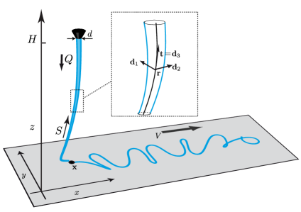
This system was first studied experimentally by Chiu-Webster and Lister Chiu-Webster and Lister (2006) (henceforth CWL), who called it the ‘fluid mechanical sewing machine’ on account of the stitch-like patterns traced on the belt by the thread. The complexity and diversity of these patterns testifies to a rich nonlinear dynamics and bifurcation structure. The appeal of the system is further increased by the theoretical and numerical challenges involved in modeling it.

In CWL’s experiments, viscous fluid (corn syrup) with density $\rho$, surface tension coefficient $\gamma$ and viscosity $\nu$ was ejected at a volumetric rate $Q$ from a vertical nozzle of diameter $d$, from which it fell a distance $H$ onto a belt moving at speed $V$ (fig. 1). The experiments were conducted by varying $V$ and $H$ for several different combinations of values of $d$, $Q$ and $\nu$. When $V$ greatly exceeded a fall height-dependent critical value $V_{b}(H)$, the fluid thread had the form of a steady dragged catenary. As the belt speed was decreased towards $V_{b}$, the lowermost part of the thread evolved into a backward-facing ‘heel’, which became unstable to periodic meandering when $V=V_{b}$. Further decrease of the belt speed led to a series of bifurcations to more complex patterns (fig. 5), ending with the establishment of steady coiling for $V=0$. CWL successfully predicted the shape of the steady dragged catenary using a ‘viscous string’ model that neglected bending stresses. However, this solution ceases to exist when the extensional axial stress at the bottom of the thread becomes zero, corresponding to the incipient formation of a heel in which the axial stress is compressional. Because a state of axial compressive stress is a necessary condition for the buckling of a slender body Taylor (1968), CWL interpreted the onset of meandering as a buckling instability of the heel.

Ribe et al. Ribe et al. (2006) carried out a numerical linear stability analysis of the dragged catenary state to predict the critical belt speed $V_{b}$ and the frequency $\omega_{b}$ for the onset of meandering, using a more complete ‘viscous rod’ theory incorporating bending and twisting of the filament. The numerical predictions of $V_{b}$ and $\omega_{b}$ thereby obtained agree closely with the experimental measurements of Chiu-Webster and Lister (2006). Ribe et al. Ribe et al. (2006) also documented a close correspondence between incipient meandering and finite-amplitude steady coiling on a motionless ($V=0$) surface, such that $\omega_{b}$ is nearly identical to the steady coiling frequency $\Omega_{c}$ for any given fall height $H$. Moreover, the critical belt speed $V_{b}(H)$ is nearly identical to the vertical (free-fall) speed $U_{f}$ of the fluid at the bottom of the thread, indicating that meandering sets in when the belt is no longer moving fast enough to carry away in a straight line the fluid falling onto it.

More extensive experiments were conducted by Morris et al. Morris et al. (2008), using a carefully engineered apparatus with silicone oil as the working fluid for better stability and reproducibility. They determined a complete phase diagram for the patterns as a function of $H$ and $V$ for a particular set of values of the fluid viscosity $\nu$ and the flow rate $Q$. They showed that the observed amplitude of meandering as a function of the belt speed is consistent with a Hopf bifurcation, and proposed a simple model to predict it based on the hypothesis that the contact point moves at constant speed relative to the belt. Finally, they proposed a generic set of amplitude equations which they used to characterize the alternating loops (which they called ‘figure-of-eight’) and translated coiling patterns.

Most recently, Blount and Lister Blount and Lister (2011) performed a detailed asymptotic analysis of a slender dragged viscous thread, focussing on the structure of the heel. They showed that the lowermost part of the thread can exhibit three distinct dynamical regimes depending on whether the belt speed is greater than, nearly equal to, or less than the free-fall speed $U_{f}$. Their asymptotic stability analysis of these steady states indicates that meandering sets in when the horizontal reaction force at the belt begins to be slightly against the direction of belt motion, corresponding to the heel ‘losing its balance’.

As the above summary indicates, our current theoretical understanding of the fluid-mechanical sewing machine is essentially limited to the initial bifurcation from the steady dragged configuration to meandering. In this paper, we push forward into the fully nonlinear regime with the help of a new computational algorithm Bergou et al. (2010); Audoly et al. (2011) that permits for the first time robust numerical modeling of arbitrary non-stationary dynamics of viscous threads. After describing the method briefly, we use it to generate a complete phase diagram of sewing-machine patterns that reproduces all the major features of the diagram determined experimentally by Morris et al. Morris et al. (2008). We then perform a detailed Fourier analysis of the motion of the contact point for each of the patterns simulated, and propose a new classification of them based on the spectral content of the motions of the contact point in two orthogonal directions.

For most of the patterns studied, we find that the frequencies present in the spectra of the contact point motion are multiples of the steady coiling frequency $\Omega_{c}$, indicating that the dynamics of the sewing machine are closely related to those of steady coiling. Accordingly, we set the stage for our study with a brief summary of the latter in the next section.

I.2 Steady coiling

In steady coiling, the contact point of the thread with the surface moves with a constant angular velocity $\Omega_{c}$ along a circle of radius $R_{c}$ (Figure 2a).

Figure 2: Steady coiling of a viscous thread. (a) Definition sketch. (b) Coiling frequency as a function of height for the parameters of the experiments of Morris et al. Morris et al. (2008), calculated numerically using a continuation method Ribe (2004). The solid curve includes the effect of surface tension ($\Pi_{3}=1.84$), while the dashed curve is for zero surface tension ($\Pi_{3}=0$). The portions of the curves corresponding to the gravitational (G), inertio-gravitational (IG), and inertial (I) regimes are indicated. The dotted lines show the first three eigenfrequencies of a free viscous pendulum.

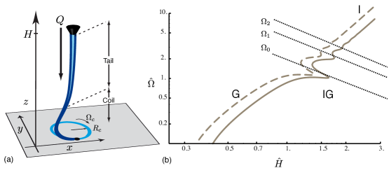
In most cases, the thread comprises two distinct parts: a long, roughly vertical ‘tail’ which deforms primarily by stretching under gravity, and a helical ‘coil’ in which the deformation is dominated by bending and (to a lesser extent) twisting. Thus the radius of the thread within the coil $a_{1}$ is nearly constant. By conservation of mass, the axial speed of the fluid in the coil is $U_{1}=Q/\pi a_{1}^{2}$.

Steady coiling can occur in several distinct dynamical regimes characterized by different balances of the viscous, gravitational, and inertial forces acting on the thread Mahadevan et al. (1998); Ribe (2004); Ribe et al. (2006). These regimes appear clearly on plots of the coiling frequency vs. the fall height. For convenience, we define a dimensionless fall height $\hat{H}$ and a dimensionless coiling frequency $\hat{\Omega}$:

$$\hat{H}=H\left(\frac{g}{\nu^{2}}\right)^{1/3},\quad\hat{\Omega}=\Omega\left(\frac{\nu}{g^{2}}\right)^{1/3}.$$ (1)

Figure 2b shows $\hat{\Omega}$ as a function of $\hat{H}$ for the parameters of the experiments of Morris et al. Morris et al. (2008), viz., $\nu=0.0277\,\mathrm{m}^{2}\,\mathrm{s}^{-1}$, $\rho=10^{3}\,\mathrm{kg\,m}^{-3}$, $\gamma=0.0215\,\mathrm{N\,m}^{-1}$, $d=8\,\mathrm{mm}$ and $\rho\,Q=0.0270\,\mathrm{g\,s}^{-1}$. For $\hat{H}<1.2$, coiling occurs in a gravitational (G) regime. Inertia is negligible everywhere in the thread, which is governed by a balance between gravity and the viscous forces that resist stretching (in the tail) and bending (in the coil). At intermediate heights $1.2\leq\hat{H}\leq 2.2$, a complex inertio-gravitational (IG) regime appears, in which the coiling frequency is a multivalued function of the fall height. The centrifugal force now becomes important in the tail, which behaves as a distributed pendulum with an infinity of eigenmodes whose corresponding eigenfrequencies are proportional to the simple pendulum frequency $(g/H)^{1/2}$. The first three of these frequencies are shown by the dotted lines in Figure 2b. When one of these eigenfrequencies is close to the frequency set by the coil, the tail enters into resonance with the latter, giving rise to resonance peaks that appear as rightward-facing ‘bumps’ in the curve $\hat{\Omega}(\hat{H})$. For large heights $\hat{H}>2.2$, coiling occurs in an inertial (I) regime in which the viscous bending force in the coil is balanced by inertia Mahadevan et al. (1998). The tail in this regime is almost perfectly vertical, and is controlled by a balance between gravity, the viscous stretching force, and the axial momentum flux. Finally, there is also a viscous (V) regime in which both gravity and inertia are negligible everywhere in the thread, but this is only observed when both $H$ and $d$ are much smaller than in the experiments of CWL and Morris et al.

In a typical laboratory experiments on steady coiling, the parameters $d$ and $Q$ and the fluid properties $\rho$, $\nu$ and $\gamma$ are held fixed while $H$ is varied. Each such experiment is completely defined by the values of the three dimensionless groups

$$\Pi_{1}=\left(\frac{\nu^{5}}{g\,Q^{3}}\right)^{1/5},\quad\Pi_{2}=\left(\frac{\nu\,Q}{g\,d^{4}}\right)^{1/4},\quad\Pi_{3}=\frac{\gamma\,d^{2}}{\rho\,\nu\,Q}$$ (2)

As an example, $\Pi_{1}=610$, $\Pi_{2}=0.370$, and $\Pi_{3}=1.84$ for all the experiments of Morris et al. Morris et al. (2008). The (dimensionless) functional dependence of the coiling frequency on the other parameters now takes the general form

$$\hat{\Omega}=\hat{\Omega}(\hat{H},\Pi_{1},\Pi_{2},\Pi_{3}).$$ (3)

The effect of surface tension is measured by the parameter $\Pi_{3}$. Surface tension modifies the coiling frequency quantitatively but introduces no essentially new dynamics, as can be seen by comparing the solid ($\Pi_{3}=1.84$) and dashed ($\Pi_{3}=0$) curves in Fig. 2b.

The continuation method used to generate the curves in Fig. 2b can be used for steady coiling because the flow is stationary in a co-rotating reference frame that moves with the contact point. No such reference frame exists for the sewing machine configuration. We therefore require a different numerical method, which is described in the next section.

II Numerical method

Our numerical experiments of the sewing machine were set up using the computational method of Discrete Viscous Threads (henceforth DVT) originally described in a conference paper Bergou et al. (2010), and presented in detail in a recent paper Audoly et al. (2011). To the best of our knowledge, DVT is the only available numerical method that is fast and robust enough to be applicable to the sewing machine geometry while retaining all the relevant modes of deformation, namely stretching, twisting and bending. For a thin thread the stretching modulus varies as the square of the thread’s radius, while the bending and twisting moduli are proportional to the fourth power of the radius. As a result the dynamics of thin threads is a nonlinear and numerically stiff problem. The DVT method addresses this difficulty by introducing an elaborate spatial discretization of the equations based on ideas from differential geometry. The method allows simulations to be run for arbitrary mesh sizes, even very coarse ones, with optimal stability. This contrasts with conventional discretization schemes which are typically stable for sufficiently small mesh sizes only, the maximum mesh size being in practice a small fraction of the smallest length scale in the flow, here the small size of the coiled region at the bottom.

Below we briefly present the principles of the DVT method, introduce adaptive mesh refinement which provides a tremendous speed-up of the calculations when gravity stretches the tail significantly, validate the code against known solutions for steady coiling, explain the details of the numerical procedure, and finally present our numerical results.

II.1 Smooth case: the equations for thin viscous threads

The numerical code makes use of the Lagrangian approach and the viscous thread is discretized as a polygonal line. A mass is assigned to each vertex, forces are set up on these masses, and the motion of each mass is obtained by time integration of the fundamental law of dynamics. The discrete forces are designed in such a way that the motion of the polygonal line is equivalent to that of a thin viscous thread in the smooth limit. The key element of the numerical method is the expressions for these discrete viscous forces. To prepare the derivation, we start by reformulating the smooth case, usually expressed in Eulerian variables, in the Lagrangian framework. We introduce a Lagrangian coordinate $S$ that marks cross-sections and follows them during motion. This Lagrangian coordinate $S$ is defined as the arc-length in an imaginary reference configuration where the thread is a cylindrical tube of constant radius. It plays the same role as the vertex index $i$ in the discrete case.

At a particular time $t$, the configuration of the thread is defined by its center-line $\mathbf{r}(S,t)$ and an orthonormal triad $(\mathbf{d}_{1}(S,t),\mathbf{d}_{2}(S,t),\mathbf{d}_{3}(S,t))$. This triad allows one to keep track of twisting, because the directions of $\mathbf{d}_{1}$ and $\mathbf{d}_{2}$ follow the orientation of a cross-section as it spins about the center-line. Thin threads deform is such a way that cross-sections remain approximately planar and perpendicular to the centerline. As a result, the center-line tangent $\mathbf{r}^{\prime}(S,t)=\frac{\partial\mathbf{r}}{\partial S}$ and the unit vector $\mathbf{d}_{3}(S,t)$ are aligned. Denoting by $\ell(S,t)$ the axial stretch factor based on the reference configuration, given by the norm of $\mathbf{r}^{\prime}(S,t)$, we have:

$$\mathbf{r}^{\prime}(S,t)=\ell(S,t)\,\mathbf{d}_{3}(S,t)\textrm{.}$$ (4)

Since the triad $(\mathbf{d}_{i}(S,t))_{i=1,2,3}$ is orthonormal, its time evolution defines a rigid-body rotation for any particular value of $S$. The associated instantaneous angular velocity ${\bm{\omega}}(S,t)$ is such that

$$\frac{\partial\mathbf{d}_{i}(S,t)}{\partial t}={\bm{\omega}}(S,t)\times\mathbf{d}_{i}(S,t)\quad\textrm{($i=1,2,3$)}\textrm{.}$$ (5)

One can take advantage of the fact that the vectors $\mathbf{r}^{\prime}$ and $\mathbf{d}_{3}$ must remain aligned by equation (4) to capture the twisting motion of the thread using a single parameter, the angular spinning velocity $w(S,t)$ defined by $w(S,t)={\bm{\omega}}(S,t)\cdot\mathbf{d}_{3}(S,t)$. In this view, which we call the centerline/spin representation Audoly et al. (2011), the material velocity ${\bm{\omega}}$ is a secondary variable which can be reconstructed by the equation

$${\bm{\omega}}(S,t)=\mathbf{d}_{3}(S,t)\times\dot{\mathbf{d}}_{3}(S,t)+w(S,t)\,\mathbf{d}_{3}(S,t)\textrm{.}$$ (6)

where the time derivative $\frac{\partial}{\partial t}$ is denoted using a dot. In a viscous thread, the fundamental kinematical quantities are the strain rates, defined by

$$\dot{\epsilon}_{\mathrm{s}}=\frac{1}{\ell}\,\frac{\partial\mathbf{u}(S,t)}{\partial S}\cdot\mathbf{d}_{3}(S,t),\qquad\dot{{\bm{\epsilon}}}_{\mathrm{tb}}=\frac{1}{\ell}\,\frac{\partial{\bm{\omega}}(S,t)}{\partial S}$$ (7)

where $\mathbf{u}=\dot{\mathbf{r}}$ is the center-line velocity. Here $\dot{\epsilon}_{\mathrm{s}}$ captures the strain rate associated with axial stretching, while the vector $\dot{{\bm{\epsilon}}}_{\mathrm{tb}}$ captures in a combined manner the strain rates for the twisting and bending modes. The strain rate for stretching, $\dot{\epsilon}_{\mathrm{s}}$, is related to the time evolution of center-line stretch $\ell$ by the formula $\dot{\epsilon}_{\mathrm{s}}=\partial\ln\ell/\partial t$.

For a thin thread, the internal stress is described by the resultant $\mathbf{n}(S,t)$ of the viscous forces over a particular cross-section, and their moment $\mathbf{m}(S,t)$ with respect to the origin of the cross-section. These internal force and moment vectors play the same role as the tensor ${\bm{\sigma}}$ in 3D continuum mechanics. For the special case of a thin thread geometry, Stokes’s constitutive law states that stress is proportional to the rate of deformation: for the stretching mode, we have

$$\mathbf{n}(S,t)\cdot\mathbf{d}_{3}(S,t)=3\,\mu\,A\,\dot{\epsilon}_{\mathrm{s}}\textrm{,}$$ (8)

and for the bending and twisting modes,

$$\mathbf{m}(S,t)=\left(3\mu\,I\,\mathbf{P}_{12}+2\mu\,I\,\mathbf{P}_{3}\right)\cdot\dot{{\bm{\epsilon}}}_{\mathrm{tb}}\textrm{.}$$ (9)

Here $\mu\equiv\rho\,\nu$ is the dynamic viscosity, $A=\pi\,a^{2}$ the cross-sectional area, $I=\pi\,a^{4}/4$ is the moment of inertia, $a$ is the radius, $\mathbf{P}_{3}=\mathbf{d}_{3}\otimes\mathbf{d}_{3}$ is the tangent projection operator, and $\mathbf{P}_{12}=\mathbf{1}-\mathbf{P}_{3}$ is the normal projection operator. The radius $a(S,t)$ is a dependent variable which is reconstructed by the incompressibility condition

$$a(S,t)=\frac{a_{0}}{\sqrt{\ell(S,t)}}\textrm{,}$$ (10)

where $a_{0}=d/2$ is the radius in the configuration of reference (note that $\ell=1$ in the reference configuration by definition). The stretching modulus $3\mu\,A$ was originally derived by Trouton Trouton (1906), and the bending modulus $3\mu\,I$ can be found for instance in Buckmaster et al. (1975).

These equations are complemented by the balance of linear and angular momentum, known as the Kirchhoff equations for thin rods:

$$\frac{\partial\mathbf{n}(S,t)}{\partial S}+\mathbf{P}(S,t) =\rho\,A_{0}\,\frac{\partial{}^{2}\mathbf{r}(S,t)}{\partial t^{2}}$$ (11)

$$\frac{\partial\mathbf{m}(S,t)}{\partial S}+\frac{\partial\mathbf{r}(S,t)}{\partial S}\times\mathbf{n}(S,t) =\mathbf{0}\textrm{.}$$ (12)

Following an approximation introduced by Kirchhoff himself which is valid for thin threads, we have neglected the rotational inertia in the second equation. The vector $\mathbf{P}(S,t)$ is the resultant of the external forces per unit reference length $\mathrm{d}S$. The weight of the thread and the surface tension are taken into account by setting

$$\mathbf{P}=\rho\,A_{0}\,\mathbf{g}-\frac{\partial(\pi\,\gamma\,a(S,t)\,\mathbf{d}_{3}(S,t))}{\partial S}$$ (13)

where $A_{0}=\pi\,{a_{0}}^{2}$ is the cross-sectional area in the reference configuration, $\mathbf{g}$ the acceleration of gravity, and $\gamma$ is the surface tension at the fluid-air interface. The last term in equation (13) is the net force on the center-line due to surface tension at the fluid-air interface, the argument in the derivative being the axial force due to the capillary overpressure $(\pi\,a^{2})\,(\frac{\gamma}{a})$. Note that there is no need to consider a linear density of applied torque in equation (12) for the problem at hand.

With suitable boundary conditions, the set of partial differential equations (4–12) constitutes a well-posed mathematical problem governing the dynamics of a viscous thread.

II.2 A variational view: Rayleigh potentials

The equations of motion (11–12) and the constitutive law (8–9) can be discretized in a natural manner Audoly et al. (2011) if they are first re-written in terms of a Rayleigh potential. The Rayleigh potential $\mathcal{D}$ yields the power dissipated by viscous forces as a function of the vertex velocity $\mathbf{u}(S)=\dot{\mathbf{r}}(S)$ and spinning velocity $w(S)={\bm{\omega}}(S)\cdot\mathbf{d}_{3}(S)$. For a thin thread, it has three contributions corresponding to the stretching, bending and twisting modes, $\mathcal{D}(\mathbf{u},w)=\mathcal{D}_{\mathrm{s}}(\mathbf{u})+\mathcal{D}_{\mathrm{t}}(\mathbf{u},w)+\mathcal{D}_{\mathrm{b}}(\mathbf{u},w)$. Note that the Rayleigh potential $\mathcal{D}$ also depends on the current configuration $\mathbf{r}(S,t)$ but this dependence will be implicit in our notations. As an illustration, consider the stretching contribution $\mathcal{D}_{\mathrm{s}}$. It only depends on the vertex velocities, and reads

$$\mathcal{D}_{\mathrm{s}}(\mathbf{u})=\frac{1}{2}\,\int 3\,\mu\,A\,(\dot{\epsilon}_{\mathrm{s}})^{2}\,\ell\,\mathrm{d}S$$ (14)

where $\dot{\epsilon}_{\mathrm{s}}$ in the integrand is given by equation (7), and $\ell\,\mathrm{d}S$ is the infinitesimal arc-length in current configuration. The expressions for the twist and bending contributions can be found in reference Audoly et al. (2011).

The Rayleigh dissipation potential is useful as it captures the effect of the internal viscous stress in a compact mathematical form. Indeed in the equations of motion (11–12) the net viscous force $\mathbf{n}^{\prime}$ and the net viscous moment $\mathbf{m}^{\prime}+\mathbf{r}^{\prime}\times\mathbf{n}$ in the left-hand sides can be shown to be equivalent to a density of applied force

$$\mathbf{P}_{\mathrm{v}}(S,t)=-\left.\frac{\partial\mathcal{D}(\hat{\mathbf{u}},\hat{w})}{\partial\hat{\mathbf{u}}(S)}\right|_{(\hat{\mathbf{u}}=\dot{\mathbf{x}}(t),\hat{w}=w(t))}$$ (15)

and a density of applied twisting torque

$$Q_{\mathrm{v}}(S,t)=-\left.\frac{\partial\mathcal{D}(\hat{\mathbf{u}},\hat{w})}{\partial\hat{w}(S)}\right|_{(\hat{\mathbf{u}}=\dot{\mathbf{x}}(t),\hat{w}=w(t))}\textrm{.}$$ (16)

In these equations, the right-hand sides denote functional derivatives, as the dissipation potential $\mathcal{D}$ takes the functions $\hat{\mathbf{u}}(S)$ and $\hat{w}(S)$ as arguments. The hat notation expresses the fact that the derivatives have to be calculated formally first, and evaluated with using the real motion $(\mathbf{u}=\dot{\mathbf{r}},w)$ next.

II.3 Discretization

In the discrete case, the center-line of the thread is represented by a polygonal chain of $n+2$ particles $\mathbf{R}(t)=\{\mathbf{r}_{0}(t),\mathbf{r}_{1}(t),\cdots,\mathbf{r}_{n+1}(t)\}$. The length $\ell^{i}(t)$ and unit tangent $\mathbf{d}_{3}^{i}(t)$ of an edge $i$ are defined by

$$\mathbf{r}_{i+1}(t)-\mathbf{r}_{i}(t)=\ell^{i}(t)\,\mathbf{d}_{3}^{i}(t)\textrm{.}$$ (17)

We consider viscous threads having a circular cross-section. As a result there is no need to keep track of the absolute orientation of the cross-sections during motion. Twist is taken into account through the instantaneous angular velocity of spin of an edge, noted $w^{i}(t)$. This is an unknown of the motion, for which we will derive an equation. Representing rotations by a single degree of freedom is beneficial for the simulation. The angular velocity vector ${\bm{\omega}}^{i}$ is a secondary quantity in the simulation, which is reconstructed from the spinning velocity $w^{i}$ by an equation similar to the smooth equation (6).

The generalized velocity of a viscous thread is obtained by complementing the vertex velocities $\dot{\mathbf{R}}(t)=\{\dot{\mathbf{r}_{0}}(t),\cdots\}$ with the spinning velocities of the edges $\mathbf{W}(t)=\{w^{0}(t),\cdots\}$. The dynamics of the thread is specified by a differential equation involving the position $\mathbf{R}(t)$, velocities $\dot{\mathbf{R}}(t)$, $\mathbf{W}(t)$, as well as the acceleration $\ddot{\mathbf{R}}(t)$. Rotational inertia is neglected and so $\dot{\mathbf{W}}(t)$ does not enter into the equation. This differential equation is derived next.

As in the smooth case, internal viscous stress is captured by means of a discrete Rayleigh dissipation potential which is the sum of three contributions, $\mathcal{D}(\mathbf{U},\mathbf{W})=\mathcal{D}_{\mathrm{s}}(\mathbf{U})+\mathcal{D}_{\mathrm{t}}(\mathbf{U},\mathbf{W})+\mathcal{D}_{\mathrm{b}}(\mathbf{U},\mathbf{W})$. As an illustration, the stretching contribution is defined in close analogy with equation (14) by

$$\mathcal{D}_{\mathrm{s}}(\mathbf{U})=\frac{1}{2}\,\sum D^{i}\,(\dot{\epsilon}_{\mathrm{s}}^{i})^{2}$$ (18)

where $D^{i}=3\,\mu\,A^{i}\,\ell^{i}$ is a discrete stretching modulus defined by analogy with equation (8), and $\dot{\epsilon}_{\mathrm{s}}^{i}=\frac{1}{\ell^{i}}\,\mathbf{d}_{3}^{i}\cdot(\mathbf{u}_{i+1}-\mathbf{u}_{i})$ is a discrete axial strain rate defined by analogy with equation (7). For an expression of the twist and bending contributions $\mathcal{D}_{\mathrm{t}}$ and $\mathcal{D}_{\mathrm{b}}$, we refer the reader to Audoly et al. (2011). They make use of discrete notions of curvature and twist, based on ideas from discrete differential geometry.

In analogy with the smooth case, we write the equations of motion as

$$\mathbf{P}_{\mathrm{v}}(t)+\mathbf{P}(t) =\mathbf{M}\cdot\ddot{\mathbf{R}}(t)$$ (19)

$$\mathbf{Q}_{\mathrm{v}}(t) =\mathbf{0}\textrm{.}$$ (20)

The first equation is a balance of linear momentum for the vertices and is associated with the positional degrees of freedom $\mathbf{R}(t)$, while the second equation is a balance of twisting torque at each edge, associated with the spinning degrees of freedom $\mathbf{W}(t)$. Here, $\mathbf{M}$ is the diagonal matrix filled with the mass of the vertices, $\mathbf{P}_{\mathrm{v}}$ and $\mathbf{Q}_{\mathrm{v}}$ are the viscous forces and twisting torques representing the internal stress in the thread, and $\mathbf{P}$ combines the weight and the net force on vertices due to surface tension. For a detailed derivation of the discrete surface tension forces, see Audoly et al. (2011). As in equation (12) for the smooth case, we have neglected rotational inertia in the right-hand side of equation (20): we have checked that this has negligible effect on the simulation when the thread is thin enough.

Our discretization of the thread is based on the Rayleigh potentials, and the discrete viscous forces and moments are defined as in equations (15) and (16) by:

$$\mathbf{P}_{\mathrm{v}}(t) =-\left.\frac{\partial\mathcal{D}(\hat{\mathbf{U}},\hat{\mathbf{W}})}{\partial\hat{\mathbf{U}}}\right|_{(\hat{\mathbf{U}}=\dot{\mathbf{R}}(t),\hat{\mathbf{W}}=\mathbf{W}(t))}$$ (21)

$$\mathbf{Q}_{\mathrm{v}}(t) =-\left.\frac{\partial\mathcal{D}(\mathbf{U},\mathbf{W})}{\partial\mathbf{W}}\right|_{(\hat{\mathbf{U}}=\dot{\mathbf{R}}(t),\hat{\mathbf{W}}=\mathbf{W}(t))}\textrm{.}$$ (22)

The equations of the present section provide a complete system of equations for the dynamics of a discrete viscous thread. For the time discretization, we use a semi-implicit Euler scheme, which provides good stability even for quite large time-steps (by semi-implicit, we mean that we linearize the equations near the current configuration at every time-step, before applying an implicit scheme). The treatment of boundary conditions is explained in section II.5.

II.4 Adaptive mesh refinement

The DVT method uses a Lagrangian grid which is advected by the flow. In sewing machine experiments, gravity can typically stretch the centerline by a factor 5 to 10 over the course of the descent. In the absence of refinement, this makes the grid very inhomogeneous: to capture the small-scale features near the belt one has to use an extremely fine mesh size near the nozzle. Overall, a large number of degrees of freedom are required and the simulation is inefficient. In addition, important inhomogeneities in edge lengths makes the time-stepping problem ill-conditioned and robustness is affected. To overcome these difficulties, we have set up adaptive mesh refinement.

In our implementation of refinement, edges are subdivided whenever their length exceeds a nominal length, which is a prescribed function of the distance to the belt. In the upper part of the belt, this nominal length is equal to twice the initial segment length, defined by the periodic release of new (Lagrangian) vertices from the nozzle. To better resolve the coil region, this nominal segment length decreased near the belt according to a prescribed exponential profile. This profile was adjusted in such a way that the coil region always includes a sufficient number of vertices, typically 10 to 30, with a final edge length typically below $0.006\,(\nu^{2}/g)^{1/3}$, and that the interval between subsequent subdivisions of a given edge is always larger than two simulation steps.

Whenever an edge was marked as needing subdivision, a new vertex was inserted. We computed the properties of the new vertex and of the two new edges as follows: the Lagrangian coordinate of the new vertex is obtained by linear interpolation, the mass stored in the former edge is equally split among its children, the position and velocity of the new vertex are calculated by an interpolation of order 4, the cross-sectional area $A$, the spinning velocities, and the viscosities of the new edges are obtained by second-order interpolation. These interpolation orders were chosen in such a way that the bending and twist forces remain continuous upon subdivision. We used the steady coiling geometry to adjust the subdivision parameters and to validate the subdivision scheme.

II.5 Emission from the nozzle, capture by the belt

We found that the implementation of boundary conditions was a key point to successfully reproduce the patterns and the phase diagram of the experimental sewing machine. We tried simple implementations first, and could reproduce the curves $\hat{\Omega}_{c}(\hat{H})$ for the frequency of steady coiling as well as the simplest stitch patterns, but failed to reproduce entire regions of the phase diagram. Further examination revealed the presence of spurious oscillations in the calculated acceleration in the steady coiling geometry ($\hat{V}=0$), even though the coiling frequency $\hat{\Omega}_{c}(\hat{H})$ was correctly predicted. We removed these spurious oscillations by a more careful account of the boundary conditions both at the nozzle and at the belt, as explained below. Suppressing these oscillations appeared to be sufficient to bring the numerical predictions in close agreement with the experimental ones.

New vertices need to be emitted periodically from the nozzle. In a first implementation of the clamped boundary conditions there, we considered an infinite string of fluid particles which were moved with the prescribed ejection velocity $Q/A_{0}$, until they passed below the nozzle and were released. The position of the first vertex clamped inside the nozzle varies abruptly as a new vertex is released, and this was the cause of unwanted oscillations. They were suppressed by considering a string of two particles in the nozzle, with a fixed position relative to the nozzle; the injection velocity is then modelled by steadily increasing the length of the second edge, and periodically inserting a new vertex in third position.

Impact with the belt was first handled by detecting penetration of vertices into the belt at the end of every time-step, and constraining their velocity to match the belt’s velocity at any subsequent time. This also induces large unwanted fluctuations in the acceleration, which can be interpreted by the fact that the vertical momentum resulting from the collision is not transferred to the thread until the following time step. The oscillations were removed by using a technique known as roll-back. Then, every time-step involves an iteration whose aim is to determine the set of vertices undergoing a collision during the time-step: whenever an unexpected collision takes place, the step is discarded, time is rolled back, and a new time-step is computed, forcing additional vertices to land on the belt at the end of the time-step. An additional difficulty in the implementation of roll-back in the context of a linearized implicit scheme, is that a only small number of particles can be captured at every step. We circumvented this difficulty by using adaptive time refinement. Such an adaptive time refinement is presumably not needed if a fully (non-linear) implicit scheme is used, such as the one presented in Ref. Bergou et al. (2010).

II.6 Validation

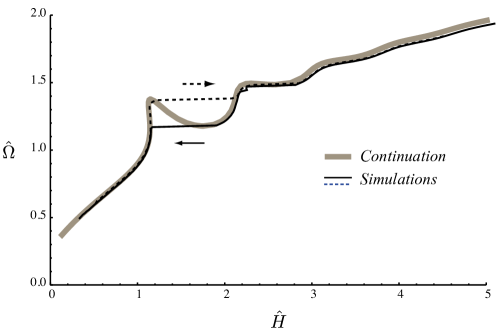
The numerical code was validated by comparing its predictions of the steady coiling frequency to the predictions of the continuation method of Ribe Ribe (2004). The agreement is excellent for all fall heights (Figure 3). The hysteresis of the dynamic simulation in the range $1.1\leq\hat{H}\leq 2.2$ is physical, but inaccessible to the continuation method because the latter records all steady-state solutions regardless of their stability.

Figure 3: Validation of the discrete numerical algorithm for a steadily coiling viscous thread with $\Pi_{1}=610$, $\Pi_{2}=0.37$, and $\Pi_{3}=0$. The discrete simulations with the fall height increasing (dashed line) and decreasing (solid line) match closely the solution of the steady-state equations obtained using an independent continuation method Ribe (2004). Arrows denote transient regimes observed in the dynamic simulation when the system jumps to a different solution branch after encountering a limit point (by contrast the continuation method records a steady but unstable solution, corresponding the part of the curve with negative slope).

III Simulation results

Our dynamic simulations of the sewing machine patterns, based on the DVT method were carried out with non-dimensional quantities. This is achieved by setting the density $\rho$, the viscosity $\mu$, and the gravity $g$ to the value 1. This choice implies that both the length scale $(\nu^{2}/g)^{1/3}$ and the time scale $(\nu/g^{2})^{1/3}$ of the problem introduced in equation (1) are equal to 1. The three other physical parameters namely the nozzle diameter, the flow rate and the surface tension were chosen to match the values of $\Pi_{1}=670$, $\Pi_{2}=0.37$ and $\Pi_{3}=1.84$ prescribed by Morris et al. experiments Morris et al. (2008): $d=0.187$, $Q=22.9\,10^{-6}$ and $\gamma=1.20\,10^{-3}$. The simulations were initiated from a vertical thread of uniform radius comprising 172 segments of equal length, falling from a height $\hat{H}=0.86$ (gravitational regime) onto a belt at rest. To avoid dealing with a shock when the thread hits the belt, the simulation was started with the bottom end of the thread clamped into the ground. The simulation was run until the radius settled to a steady profile as a function of the elevation, and a steady state of coiling was established. Next the $(\hat{H},\hat{V})$ space was sampled by slowly varying $\hat{H}$ or $\hat{V}$ in turn.

As an illustration of the capabilities of our numerical technique, we show in Figure 4 a simulation of the ’translated coiling’ pattern that occurs for relatively low belt speeds.

Figure 4: Simulation of the translated coiling pattern for $\Pi_{1}=670$, $\Pi_{2}=0.37$, $\Pi_{3}=0$, $\hat{H}=0.98\,$ and $\hat{V}=0.022$ using 182 vertices for 181 segments. (a) Three-dimensional perspective view. A–D denote reference points along the thread. (b) Thick gray curve: trajectory of the contact point in the frame of the nozzle. The velocity of the contact point relative to the belt is shown at various times (thin gray lines) and highlighted when the contact points passes the reference points A–D (green arrows) . (c) Viscous power dissipated per unit length $\mathrm{d}\mathcal{D}/\mathrm{d}\hat{s}$ by the stretching modes (plain black and dashed black curves, respectively), and by the twisting and bending modes (thick grey curve), as a function of arc-length $\hat{s}$, when the contact point passes the apical reference position C. All numerical quantities are dimensionless, as explained in the beginning of section III.

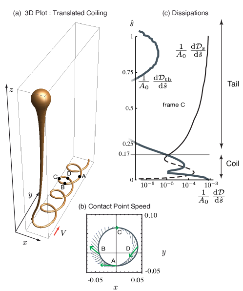
Fig. 4a shows a three-dimensional view of the falling thread and the trace it lays down on the belt. The simulation time is $0.73\;\mathrm{s}$ for one period of this pattern using a $2.6\;\mathrm{Ghz}$ Intel Core i7 processor and $8~{}\mathrm{Go}$ of $1067\;\mathrm{Mhz}$ DDR3 memory.

Fig. 4b shows the trajectory of the contact point in the frame of the nozzle (solid line). Interestingly, the belt motion breaks the symmetry of steady coiling not only in the longitudinal $x$-direction, but also in the transverse $y$-direction. Fig. 4b also shows the velocity of the contact point relative to the moving belt as a function of position along the trajectory (thin lines and green arrows). The magnitude of the relative velocity varies significantly over a period, in contrast to the meandering pattern for which it is nearly uniform Morris et al. (2008). The relative speed is maximum at point A where the contact point is moving upstream along the belt, and very small at C where the motion is downstream. Finally, fig. 4c shows the amount of viscous power dissipated by the various modes, as a function of arc-length along the thread. The curves cross each other at a height $z\approx 0.1$ that corresponds to the transition from the bending-dominated coil, to the stretching-dominated tail. Thanks to adaptivity, the coil is well resolved and the curves for the viscous power dissipation remain smooth there, even though they vary rapidly.

In addition to the dimensionless parameters $\Pi_{1}$, $\Pi_{2}$ and $\Pi_{3}$ in equation (2) that describe the fluid properties and the ejection conditions, the patterns depend on the dimensionless fall height $\hat{H}$ in equation (1), and the dimensionless belt speed

$$\hat{V}=V(\nu g)^{-1/3}.$$ (23)

Our simulations were carried out by varying $\hat{H}$ and $\hat{V}$ for fixed values of $\Pi_{1}=610$ and $\Pi_{2}=0.370$ corresponding to the experiments of Morris et al.Morris et al. (2008). Some of our simulations were done with a surface tension parameter matching the experimental value $\Pi_{3}=1.84$; for reasons of numerical stability, however, most of the simulations used $\Pi_{3}=0$.

Figure 5 summarizes all the types of patterns that were encountered when scanning the ($\hat{H},\hat{V}$) plane in the simulations, together with their experimental equivalents Chiu-Webster and Lister (2006).

Figure 5: Simulated sewing machine patterns (black curves) together with photographs of similar patterns observed experimentally Chiu-Webster and Lister (2006). The comparison is qualitative because the parameters used in the simulations ($\Pi_{1}=670$, $\Pi_{2}=0.37$, $\Pi_{3}=0$) are not the same as in the experiments of Chiu-Webster and Lister (2006). A: Transient coiling, B: Meanders, C: Alternating loops (figure-of-eight) pattern, D: Disorder, E: Double coiling, F: Double meanders, G: W pattern, H: Stretched coiling, I: catenary. (^∗) Photo Courtesy: Chiu-Webster and Lister.

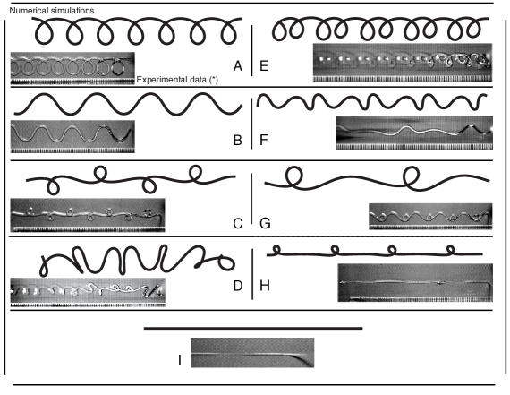
The simulation reproduces nine out of the ten patterns reported by Morris et al.Morris et al. (2008) and observed by CWL Chiu-Webster and Lister (2006). The only missing pattern, the slanted loops, will be discussed later on. To ease the understanding, the name ’figure-of-8’ is replaced by ’alternating loops’ which more accurately describes the pattern in Figure 5C.

In Figure 6 a phase diagram lists all the numerical patterns encountered in the $(\hat{H},\hat{V})$ space for $\hat{H}\leq 0.8$.

Figure 6: Phase diagram of the numerically simulated patterns as a function of dimensionless fall height $\hat{H}\leq 0.80$ and dimensionless belt speed $\hat{V}$, for $\Pi_{1}=670$, $\Pi_{2}=0.37$ and $\Pi_{3}=1.84$. The observations of Morris et al. Morris et al. (2008) are shown by colored dots for comparison. The typical appearance of each pattern (catenary, meanders, alternating loops, translated coiling) is shown in insets.

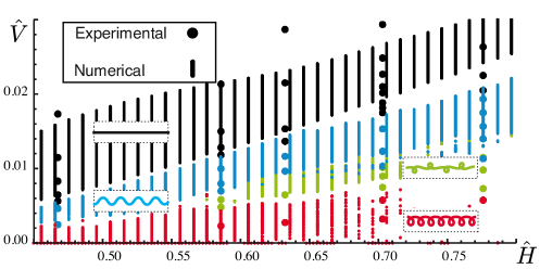
The effect of surface tension is included, $\Pi_{3}=1.84$ in the simulation. For comparison, the patterns observed experimentally by Morris et al.Morris et al. (2008) are shown by dots. The agreement between the simulations and the experiments is remarkable: all four patterns that were observed experimentally in this region of the parameter space, namely translated coiling, alternating loops, meanders and catenary, are recovered. In addition the location of the boundaries separating the different patterns are reproduced accurately.

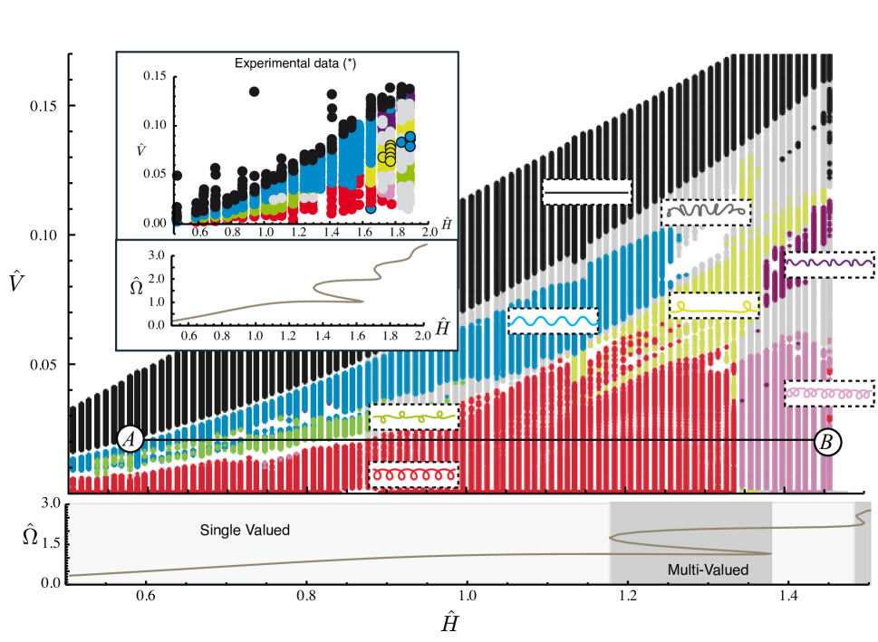
The inclusion of surface tension gives rise to numerical instabilities for heights approximately above $\hat{H}>0.70$, which we have not been able to overcome by decreasing the mesh size or the time-step. This is why there is no simulation data shown in the lower right portion of Figure 6. Since surface tension is not expected to modify qualitatively the dynamics of threads (see Fig. 2) we investigated the case of larger fall heights without any surface tension ($\Pi_{3}=0$). Five new patterns were observed for larger fall heights, as shown in Figure 7, namely double coiling, double meanders, stretched coiling, W-pattern, disordered pattern, despite the absence of surface tension in the simulations. The new portion of the phase diagram, $\hat{H}>0.8$, is very similar to that reported by Morris et al.Morris et al. (2008), shown in the inset in Fig. 7. In both diagrams, the alternating loops pattern disappears at a critical height, beyond which there is a substantial height ‘window’ containing only simple patterns (catenary, translated coiling, and meanders). When the height is increased, three patterns having a complex aspect (disordered pattern, stretched coiling and the double meanders) all appear together at nearly the same height. Finally, for some values of the height, disordered patterns, shown in grey in the diagram, occur in two separate ranges of the belt speed, with stretched coiling in between.

It is instructive to compare the numerical and experimental phase diagrams with the curves $\hat{\Omega}_{c}(\hat{H})$ of frequency vs. height for steady coiling, calculated with same value of surface tension ($\Pi_{3}=0$ for the simulations, $\Pi_{3}=1.84$ for the experiments). These curves are shown below each phase diagram in Figure 7. The comparison reveals that some of the more complicated patterns (stretched coiling, W-pattern, disordered pattern) appear at heights close to that for the onset of the multivalued IG regime in the steady coiling. In the steady coiling geometry, it is known that the multivalued regime is caused by the competition of several ‘viscous pendulum’ modes. This suggests that the complex patterns of the sewing machine are produced by the non-linear interaction of these pendulum modes.

Despite their similarities, the numerical (N) and experimental (E) phase diagrams in Figure 7 exhibit some systematic differences. In E, double coiling (pink) first appears at the same height as the disordered (grey) and stretched coiling (yellow), whereas in N it appears at significantly greater heights. Double meanders (purple) have a common boundary with the catenary pattern (black) in E, but occur only for significantly lower belt speeds in N. In N, the catenary state can transition to disorder (grey) over a range of heights, unlike in E. The range of belt speeds for double coiling is significantly wider in N than in E. Finally, in N the W-pattern is observed sporadically and for greater heights than in the diagram in Fig. 7. Some of these differences are due to the absence of surface tension in the simulations, and to the fact that collisions of the viscous thread with its trace are not prevented. Another explanation for the discrepancies may be the fact that Morris et al. Morris et al. (2008) performed their pattern recognition visually, whereas we used a more quantitative automatic procedure based on Fourier decomposition. This is described in the following section, where we review each of the individual patterns in detail and propose a systematic classification of them.

Figure 7: Phase diagram of sewing machine patterns determined from numerical simulations with $\Pi_{1}=670$, $\Pi_{2}=0.37$ and no surface tension ($\Pi_{3}=0$). The patterns simulated include translated coiling (red), meanders (blue), alternating loops (green), double coiling (pink), stretched coiling (yellow), double meanders (purple), and disordered patterns (grey). The catenary pattern in black would extend all the way up in the diagram, the border between black stripes and the white region at the top being only the result of the simulation being stopped for large enough values of $\hat{V}$. The W-pattern (yellow dots circled in black in inset) and slanted loops (blue dots circled in black in inset) are discussed in section IV.2. The horizontal path AB is used to construct Figure 8. The coiling frequency $\hat{\Omega}$ for steady coiling is shown as a function of height $\hat{H}$ below the phase diagram. Inset: Phase diagram determined experimentally Morris et al. (2008) for $\Pi_{1}=670$, $\Pi_{2}=0.37$, and $\Pi_{3}=1.84$ (top) together with the corresponding curve $\hat{\Omega}(\hat{H})$ (bottom).

IV Analysis of the patterns

To illustrate our pattern analysis, we fix the belt speed $\hat{V}=0.02$ and vary the fall height, thereby following the horizontal line AB in the phase diagram of Fig. 7. In order of increasing height, the patterns seen along this line are meanders, alternating loops, translated coiling, and double coiling. We track the spectral content of these patterns continuously as they change smoothly or bifurcate. To do so, we focus on the trajectory of the contact point of the thread with the belt. Let $x(t)$ and $y(t)$ be its longitudinal and transverse coordinates in the laboratory (nozzle) reference frame, and define $\mathbf{x}(t)=x(t)+iy(t)$. Let $X(t,t^{*})$ and $Y(t,t^{*})$ be the coordinates (also relative to the nozzle) at time $t$ of a material point that was laid down on the belt at time $t^{*}<t$, and let $\mbox{\boldmath$X$}(t,t^{*})=X(t,t^{*})+i\,Y(t,t^{*})$ be a generic point in the trace. The advection by the belt is expressed by:

$$\mbox{\boldmath$X$}(t,t^{\star})=\mathbf{x}(t^{\star})+(t-t^{*})\,V.$$ (24)

This equation means that the pattern $\mbox{\boldmath$X$}(t,t^{*})$ seen on the belt is obtained by unfolding the motion of the contact point motion $\mbox{\boldmath$x$}(t)$, as illustrated in Fig. 9a.

The numerical traversal of the line AB in Figure 7 required about 78500 time steps of size $\delta t=0.1(\nu/g^{2})^{1/3}$. We performed a Fourier analysis of the motion $\mbox{\boldmath$x$}(t)$ over a sliding window of 2000 time steps (the FFT spectrum was computed every 500 steps). The spectra obtained in this way typically comprise several well-defined peaks whose frequencies can be determined precisely (Fig. 9b).

Figure 8: Frequency content of patterns encountered along the line AB through the phase diagram of Figure 7. Frequencies of transverse ($y$-direction) and longitudinal ($x$-direction) motion are shown as blue and red, respectively. Note that these frequency are the same in the upper region of the diagram where the two colors overlap. In the dashed insets, the patterns are identified using the same color codes as in Figure 7. Grey bands indicate ranges of heights for which the patterns are transient. Also shown is the frequency $\hat{\Omega}_{c}$ of steady coiling as a function of height (brown solid line), together with several multiples of that frequency (brown dotted lines).

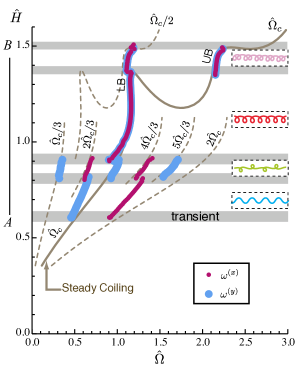
Let $\omega^{(x)}_{1}$, $\omega^{(x)}_{2}$, etc. be the peak frequencies of the motion in the $x$-direction, and $\omega^{(y)}_{1}$, $\omega^{(y)}_{2}$, etc. be those for the motion in the $y$-direction. Because the fall height $\hat{H}$ is slowly changing with time during the simulation, each observed frequency $\omega^{(x)}_{i}$ or $\omega^{(y)}_{i}$ can be plotted on a diagram to provide a ‘portrait’ of the evolving frequency content of the contact point motion, as a function of the fall height $\hat{H}$. The result is shown in Figure 8. The principal observed frequencies $\omega^{(x)}_{n}$ and $\omega^{(y)}_{n}$ are indicated in red and blue, respectively. Also shown for reference is the steady coiling frequency $\hat{\Omega}_{c}(\hat{H})$ for the same fluid properties and ejection parameters (solid line), together with several multiples (1/3, 2/3, 1/2, 4/3, 5/3, 2) of that frequency (dashed lines).

The first pattern ($0.62\leq\hat{H}\leq 0.8$) is meandering, which is characterized by two frequencies with a ratio $\omega^{(x)}_{1}/\omega^{(y)}_{1}=2$. At the lowest height $\hat{H}=0.62$ where meandering first appears, the meandering frequency $\omega^{(x)}_{1}$ is very close to the steady coiling frequency $\hat{\Omega}_{c}$ for the same height, as expected on theoretical groundsRibe et al. (2006); Blount and Lister (2011). The next pattern ($0.8\leq\hat{H}\leq 0.9$) is the alternating loops, which has a rich spectrum involving five multiples of $\hat{\Omega}_{c}/3$. Translated coiling appears next ($0.9\leq\hat{H}\leq 1.35$), and is characterized by a single frequency $\omega^{(x)}_{1}=\omega^{(y)}_{1}$ very close to the steady coiling frequency. Finally, double coiling ($1.35\leq\hat{H}\leq 1.5$) has two frequencies $\omega^{(x)}_{1}=\omega^{(y)}_{1}\approx\hat{\Omega}_{c}$ and $\omega^{(x)}_{2}=\omega^{(y)}_{2}\approx\hat{\Omega}_{c}/2$.

Figure 9: Three-stage analysis of the patterns, illustrated for the case of meandering. (a) From the trace of the thread on the belt (a1), we extract the trajectory of the contact point in the frame of the nozzle (a2). (b1) Fourier spectra of the longitudinal (red) and transverse (blue) components are obtained by Fast Fourier Transform, and compared to the frequencies $\hat{\Omega}$ of steady coiling for the same height: the blue and red dots in (b2) are the main frequencies in the simulation, while the intersection of the horizontal line with the thick black curve is the frequency of steady coiling. In the example shown here the belt speed is close to the critical value for the onset of meandering and the dominant transverse frequency $\omega_{1}^{(y)}$ is close to the steady coiling frequency $\hat{\Omega}_{c}$ for the same height. (c) The two main frequencies extracted by FFT are injected into the kinematic model (26) to generate a synthetic motion for the contact point in the nozzle frame (c1), and a synthetic stitch pattern (c2). In the example shown, the motion involves only one transverse frequency $\omega_{1}^{(y)}$ and one longitudinal frequency $\omega_{1}^{(x)}=2\omega_{1}^{(y)}$.

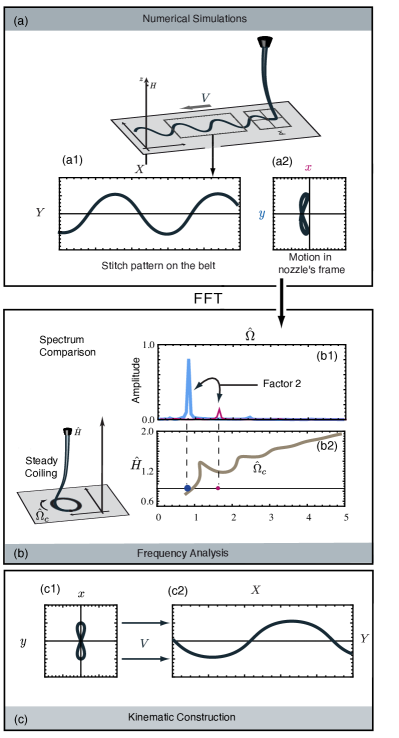
Figure 8 shows that the stitch patterns are combinations of motions in two orthogonal directions with frequencies closely related to the steady coiling frequency $\hat{\Omega}_{c}$. Accordingly, we now change our perspective and classify the patterns based on their frequency content rather than on the shape they lay down on the belt. This frequency analysis is used to set up an efficient tool for identifying the patterns and assembling the numerical phase diagram automatically. In addition it leads to a simple kinematic model that provides a unified description of the different patterns.

IV.1 Spectral signature of a pattern

We illustrate our method using the example of meandering which in most cases is the first pattern to bifurcate from the catenary state as the belt speed decreases. The red and blue lines in figure 9b show typical spectra of the motion of the contact point in the longitudinal $x$ and transverse $y$-directions, respectively. The amplitude of the transverse motion is much greater than that of the longitudinal motion, and the frequency of the latter is exactly twice that of the former, $\omega_{1}^{(x)}=2\omega_{1}^{(y)}$. This suggests that a meander pattern can be synthesized by retaining only the two main frequencies, viz.

$$\mbox{\boldmath$x$}(t)=\alpha_{1}\cos(2\omega_{1}^{(y)}t)+i\,\beta_{1}\cos(\omega_{1}^{(y)}+\pi/4)$$ (25)

where $\alpha_{1}$ and $\beta_{1}$ are the amplitudes of the longitudinal and transverse motions, respectively. Here the phase difference $\pi/4$ is required to reproduce the symmetry of the pattern. A similar two-frequency model was used by Morris et al. Morris et al. (2008) to analyze weakly non-linear meanders. Figure 9c1 shows the contact line trajectory in the frame of the nozzle implied by (25) with $\alpha_{1}/\beta_{1}=0.2$, and Figure 9c2 shows the corresponding meander pattern obtained by advecting the motion (25) in the $x$-direction with $V=1.4(\nu g)^{1/3}$ and $\omega_{1}^{(y)}=1$. Based on Figure 9, we define as a ‘meander’ any pattern whose longitudinal motion, compared to the transverse motion, has twice the frequency, a much smaller amplitude, and a phase shift of $\pi/4$.

Generalizing the above example, we show that all the sewing machine patterns can be represented by a superposition of a few harmonic motions of the form:

$$x(t)+iy(t)=\sum_{j=1}^{N_{x}}\alpha_{j}\cos(\omega^{x}_{j}t+\phi^{x}_{j})+i\sum_{j=1}^{N_{y}}\beta_{j}\cos(\omega^{y}_{j}t+\phi^{y}_{j})\textrm{.}$$ (26)

Two terms in each direction are sufficient to reproduce the main features of the patterns, $N_{x}\leq 2$ and $N_{y}\leq 2$. In Eqn. (26), $\alpha_{j}$ and $\beta_{j}$ are the amplitudes of the components of the motion with frequencies $\omega^{(x)}_{j}$ and $\omega^{(y)}_{j}$, and $\phi^{x}_{j}$ and $\phi^{y}_{j}$ are the phases relative to the highest-frequency mode. We now show how each of the sewing machine patterns can be characterized in terms of the parameters that appear in Eqn. (26).

IV.2 Identification of the patterns

The identity of each pattern is determined not by the absolute values of the parameters in Eqn. (26), but rather by the dimensionless groups that can be formed from them, namely frequency ratios, amplitude ratios, and the relative phases $\phi_{j}$. In the following we identify the characteristic values of these groups for each of the patterns in turn. For ease of reference, the results are summarized in Table 1.

Figure 10: Kinematic analysis of individual sewing machine patterns. (A) coiling; (B) alternating loops; (C) double coiling. For each pattern, the upper left, right, and lower left panels correspond to parts a), b) and c), respectively, of Figure 9. The kinematical reconstruction is a proof of concept, there is no attempt to match the wavelength of the simulations.

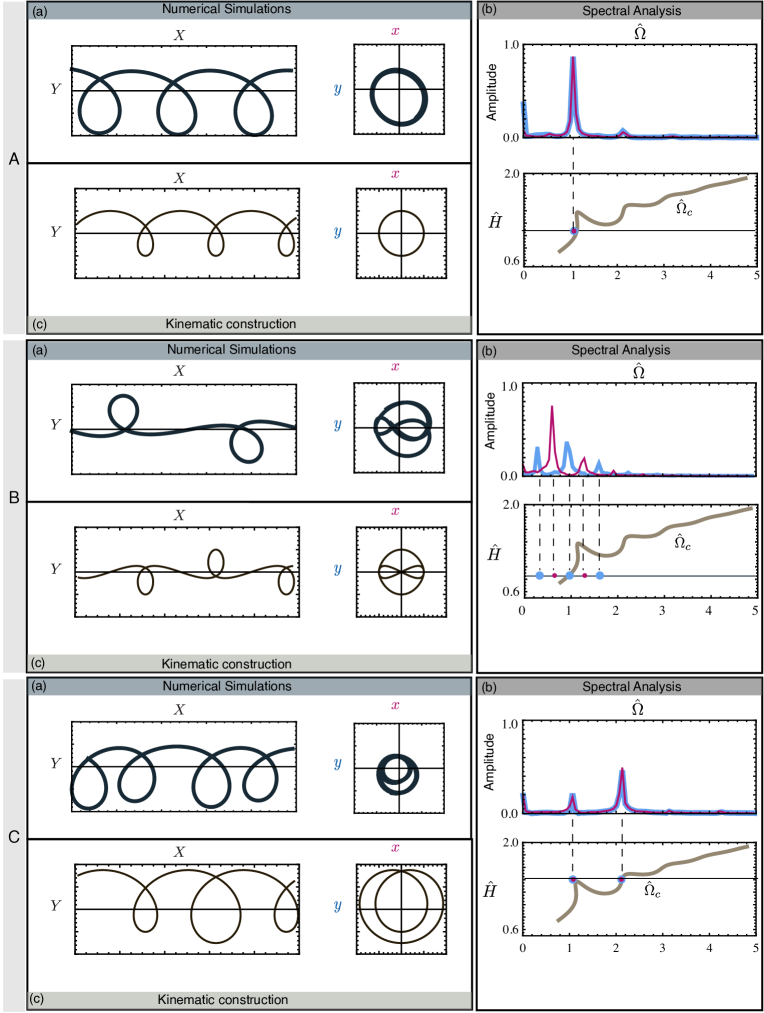
1. Translated coiling. This pattern occurs for $0.5\leqslant\hat{H}\leqslant 1.35$ and low belt speeds (Figure 7). Figure 10A shows a simulation of this pattern (upper left) and the corresponding Fourier spectra of the longitudinal and transverse motions of the contact point (upper right), and the steady coiling frequency $\hat{\Omega}_{c}$. The longitudinal and transverse motions have similar amplitudes and are characterized by a single dominant frequency $\omega_{1}^{(x)}=\omega_{1}^{(y)}$ that is very close to the steady coiling frequency $\hat{\Omega}_{c}(\hat{H})$ for the same fall height $\hat{H}$. The peak frequency deviates from its original value as the belt speed increases. The amplitudes in both directions remain equal and an almost circular shape is created. The panels at lower left show the reconstructed motion in the frame of the nozzle (right) and on the belt (left), calculated using (26) with $N_{x}=N_{y}=1$, $\alpha_{1}=\beta_{1}=1$ and $\omega_{1}^{(x)}=\omega_{1}^{(y)}=1$. Note that the experimental pattern shifts upwards or downwards as the belt speed is increased; this shift does not affect the spectral context, but could be taken into account by including a purely imaginary constant in Eqn. (26).

Patterns	$\omega_{1}^{x}$	$\omega_{2}^{x}$	$\omega_{1}^{y}$	$\omega_{2}^{y}$	$\phi_{1}^{x}$	$\phi_{2}^{x}$	$\phi_{1}^{y}$	$\phi_{2}^{y}$	$\alpha_{1}$	$\alpha_{2}$	$\beta_{1}$	$\beta_{2}$	V
Translated Coiling	$1^{*}$	-	$1^{*}$	-	0	-	0	-	1.	-	1.	-	.5
Meanders	2	-	$1^{*}$	-	0	-	$\pi/4$	-	.2	-	1.	-	1.4
Alternating loops	1	-	1/2	$3/2^{*}$	$\pi/2$	-	0	0	1	-	.5	.5	0.33
Double Coiling	1/2	$1^{*}$	1/2	$1^{*}$	$\pi/2$	$\pi/2$	0	0	.5	1.5	.1	1.5	.5
Double Meanders	1/2	-	-	$1^{*}$	$\pi/4$	-	0	-	1.	0	0	1.5	.75
Stretched Coiling	1	$2^{*}$	1	$2^{*}$	$\pi/2$	$\pi/2$	0	0	1.	.1	.5	.1	.6
W-pattern	1	$2^{*}$	1	$2^{*}$	$\pi/2$	$\pi/2$	0	0	1.	.2	.2	.5	.7
Catenary	-	-	0	-	-	-	0	-	-	-	0	-	1
Disorder	-	-	-	-	-	-	-	-	-	-	-	-	-

Table 1: Parameters of the kinematic model in Eqn. (26) used to construct synthetic patterns. Because the patterns are defined by the relative values of the frequencies $\omega_{1}^{x}$ and $\omega_{1}^{y}$, the frequency 1 is assigned by convention to the peak of largest amplitude. The other frequencies are given by ratios of small integer numbers. A star indicates a frequency that is locked to the steady coiling frequency $\hat{\Omega}_{c}$. Likewise, the amplitudes $\alpha_{1}$, $\alpha_{2}$, $\beta_{1}$ and $\beta_{2}$ are given relative to each other, and correspond to typical values. $V$ indicates the speed of the belt used to unfold the synthetic patterns. A dash indicates that the parameter is not relevant for the pattern in question. The disordered pattern is not reconstructed using the kinematical model as it involves more harmonics.

2. Meanders. On Figure 7 this pattern is seen for $0.6\leqslant\hat{H}\leqslant 1.3$ and a range of intermediate belt speeds. The typical Fourier spectra of the meandering pattern were previously shown in Figure 9. The pattern is a superposition of a single longitudinal, and a single transverse harmonic motions, with frequency ratio $\omega_{1}^{(x)}/\omega_{1}^{(y)}=2$, amplitude ratio $\alpha_{1}/\beta_{1}\ll 1$, and a relative phase $\phi_{1}^{y}=\pi/4$ (with the convention $\phi_{1}^{x}=0$). Near the catenary/meander boundary $\omega_{1}^{(y)}\simeq\hat{\Omega}_{c}$; farther from the boundary, the meandering frequency departs significantly from $\hat{\Omega}_{c}$. The regular symmetrical meanders correspond to a phase difference of $\pi/4$ between the two directions (fig. 9) However, the pattern may deform into a bean-like shape in certain cases. This situation was reproduced kinematically by reducing the phase difference to a value close to $\pi/6$.

3. Alternating loops. This pattern was called ‘figure-of-eight’ by CWLChiu-Webster and Lister (2006) and Morris et al.Morris et al. (2008), but we prefer to call it ‘alternating loops’. The domain of this pattern is an elongated ‘bubble’ sandwiched between translated coiling and meandering at relatively low fall heights $\hat{H}\leq 1$ (Figure 7). This pattern displays a remarkably rich frequency spectrum with five principal peaks (Figure 10B-c). In contrast to meandering, the motion with the largest amplitude is longitudinal, with a frequency $\omega_{1}^{(x)}$ that locks onto the frequency $2\hat{\Omega}_{c}/3$ (see also Figure 8). The next largest peaks correspond to a transverse motion with frequencies $\omega^{(y)}_{2}=\hat{\Omega}_{c}$ and $\omega^{(y)}_{1}=\hat{\Omega}_{c}/3$, both amplitudes being very close. The harmonics $4\hat{\Omega}_{c}/3$ in the longitudinal direction, and $5\hat{\Omega}_{c}/3$ in the transverse direction are also visible.

The frequencies of all five peaks can be written compactly as

$$\omega^{(y)}_{p} =(2p-1)\,\frac{\hat{\Omega}_{c}}{3} (p=1,2,3),$$

$$\omega^{(x)}_{p} =2p\,\frac{\hat{\Omega}_{c}}{3} (p=1,2).$$

Even though the spectra in Fig. 10B-b shows five peaks, the kinematic model in Eqn. (26) generates an almost identical pattern if one retains only the three main contributions $\omega_{1}^{(x)}$, $\omega_{1}^{(y)}$, and $\omega_{2}^{(y)}$ with an amplitude ratio $\beta_{1}/\alpha_{1}\approx.5$, $\beta_{1}/\alpha_{2}\approx.5$, and phases $\phi_{1}^{x}=\pi/2$ and $\phi_{1}^{y}=\phi_{2}^{y}=0$ (Figure 10B-c). We used these characteristics of the three main frequencies as a criterion for automatic detection of alternating loops.

Figure 11: Same as Figure 10, but for (A) double meanders, (B) stretched coiling, and (C) the ’W-pattern’. $\delta A$ denotes the difference of amplitude.

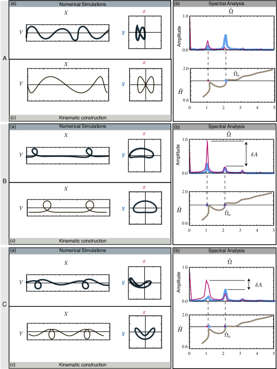
4., 5. Double coiling and double meanders. The Fourier spectra for these patterns are shown in Figures 10C and 11A, respectively. Both the longitudinal and transverse components have peaks at two frequencies $\omega_{1}^{(x)}=\omega_{1}^{(y)}=\hat{\Omega}_{c}/2$ and $\omega_{2}^{(x)}=\omega_{2}^{(y)}=\hat{\Omega}_{c}$. The origin of these frequencies is clear from the uppermost part of Figure 8, which shows them as functions of fall height for double coiling. The range of fall heights in question is within the inertio-gravitational regime of steady coiling, for which the curve $\hat{\Omega}_{c}(\hat{H})$ is multivalued in specific height ranges (Figure 2). The portion $1.2\leq\hat{H}\leq 1.5$ of that curve has two stable branches corresponding to different ‘pendulum’ modes of the tail: a lower branch (labelled LB in Figure 8) with $\hat{\Omega}_{c}\approx 1.15$, and an upper branch (UB) with $\hat{\Omega}_{c}\approx$ 2.1-2.2. Figure 8 shows that the higher double coiling frequency $\omega_{2}^{(x)}=\omega_{2}^{(y)}$ stays locked to the upper branch of $\hat{\Omega}_{c}(\hat{H})$, which is the only stable one when $\hat{H}\geq 1.37$. The lower frequency, by contrast, follows a ‘phantom’ branch with frequency $\hat{\Omega}_{c}/2$ that is very nearly a direct continuation of the lower branch of $\hat{\Omega}_{c}(\hat{H})$ to greater fall heights. This behavior is possible because the ratio of the frequencies of the upper and lower branches happens to be quite close to 2.0.

Although double coiling and double meanders have the same frequency content, they are distinguished by the relative amplitudes and phases of the transverse and longitudinal motions. For double coiling, the amplitudes of the two motions are the same at both frequencies ($\alpha_{1}=\beta_{1}$, $\alpha_{2}=\beta_{2}$), and the relative phases are $\phi_{1}^{x}=\phi_{2}^{x}=\pi/2$ and $\phi_{1}^{y}=\phi_{2}^{y}=0$. For double meandering, by contrast, the transverse motion is dominated by the frequency $\omega_{2}^{(y)}=\hat{\Omega}_{c}$ while the longitudinal motion is dominated by $\omega_{1}^{(x)}=\hat{\Omega}_{c}/2$. The relative phases are $\phi_{1}^{x}=\pi/4$ while $\phi_{1}^{y}=0$.

6., 7. Stretched coiling and the W-pattern. These patterns occur predominantly in the range of heights corresponding to inertio-gravitational coiling (right-hand side of Figure 7). Their typical Fourier spectra are shown in Figure 11B and C, respectively. Like double coiling and double meanders, their characteristic signature is the ($\hat{\Omega}_{c}/2,\hat{\Omega}_{c}$) frequency couple. But whereas double coiling and double meanders are dominated by transverse motion at the frequency $\hat{\Omega}_{c}$, stretched coiling and the W-pattern are dominated by longitudinal motion at the frequency $\hat{\Omega}_{c}/2$. The difference between stretched coiling and the W-pattern is only due to different relative amplitudes of the transverse and longitudinal motions denoted $\delta_{A}$ in Figure 11B-b and C-b. The $x-$direction is dominant in both cases but the peak at $\hat{\Omega}_{c}$ in the $y$-direction is much closer for the W-pattern than for the stretched coiling. Theses differences cause the change of invagination between the two patterns (Figure 11B-a and C-a). The phase difference between the longitudinal and transverse motions is $\pi/2$ in both cases.

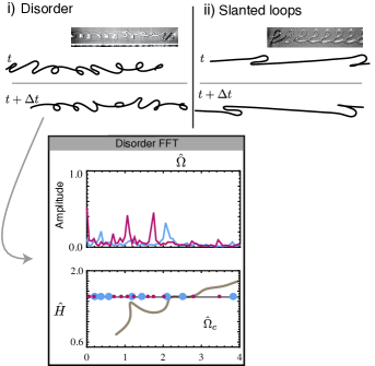
8. Disorder. Disordered patterns appear in several parts of the phase diagram (grey in Figure 7), primarily at heights within the inertio-gravitational coiling regime. The typical Fourier spectra of these patterns is very rich, with more than four peaks in both the longitudinal and transverse directions with comparable and strongly time-dependent amplitudes (Fig. 12-i and corresponding FFT). Such patterns are not transient between two steady patterns, as the aperiodic behavior persists indefinitely in time.

9. Catenary. The catenary is obtained when the point of contact is at rest in the nozzle frame, which happens in the upper region of the phase diagram. The FFT spectrum is then empty.

In addition to the patterns discussed above, slanted loops Chiu-Webster and Lister (2006) were also reported by Morris et al. Morris et al. (2008) in a very narrow region of their phase diagram. Slanted loops is a pattern wherein a buckle is periodically laid down on the belt, and subsequently closes up into a loop when the thread touches itself and coalesces. Our numerical simulations do not account for self-contact of the thread, nor for surface tension-mediated coalescence. This probably explains why we observed slanted loops transiently only, as shown in Fig. 12-ii. A similar argument may also explain why the W-pattern is observed for significantly larger fall heights in the simulations than in the experiments: considering self-contact of the thread would certainly favor its existence over the stretched coiling pattern in the simulation.

We observe that CWL Chiu-Webster and Lister (2006) reported yet another pattern, side kicks. Side kicks consist of small heaps of fluid regularly spaced along an otherwise perfectly straight trace. We suggest that this pattern is a limiting case of stretched coiling in which the amplitude of the transverse motion becomes very small relative to that of the longitudinal motion. Side kicks have not been reported in the experimental phase diagram of Morris and al., the one we attempt to reproduce in the simulations; consistently, we have observed this pattern in our simulation only transiently.

Figure 12: Unsteady patterns: (i) disordered pattern and (ii) slanted loops. Both patterns are shown at two different times of the simulations, and compared in the insets to experiments Chiu-Webster and Lister (2006). The lower part of the figure illustrates the FFT of the disordered patterns.

V Discussion

The simulations of the fluid-mechanical sewing machine presented here were performed using a new numerical algorithm, Discrete Viscous Threads (DVT). The essential idea of DVT is to start from a complete geometrical and kinematical description of the thread in the discrete setting, and push the discrete approach as far as possible; in particular a discrete representation of viscous stress is built based on a variational view (Rayleigh potentials). This approach leads to a code that is robust even for quite large mesh size. This numerical method is used to simulate complex unsteady behavior of a viscous thread and offers good efficiency. As an example, the traversal (78500 time steps) of the line AB in Figure 7 required $987\;\mathrm{s}$ on a $2.87\,\mathrm{GHz}$ Intel Core processor. The accuracy of the method is demonstrated by its ability to reproduce the curve of steady coiling frequency vs. height, as predicted by an independent continuation method (Figure 2), and by the close agreement between the calculated and experimentally determined phase diagrams for the sewing machine patterns (Figure 6).

At each time step in an unsteady DVT simulation, any desired kinematical or dynamical variable can be calculated as a function of arc-length, i. e. at every vertex along the thread’s centerline. Examination of these functions provides insights into the thread’s dynamics. We saw an example in Figure 4c, which showed the local rates of viscous dissipation of energy due to deformation by stretching (or compression), bending, and twisting. The figure reveals that the thread is divided into two distinct parts: a ‘tail’ in which the dissipation is dominated by stretching, and a ‘coil’ in which it is dominated by bending and twisting, but with a significant contribution from compression. The differential equations describing bending are of higher order than those describing stretching, so Figure 4c implies that the coil is an ‘inner’ solution or boundary layer whose presence is required by the need to satisfy all the relevant boundary conditions at the thread’s contact point with the belt. While the boundary-layer character of the coil region has long been recognized for steady coiling Mahadevan et al. (1998); Ribe (2004), our simulations open up the possibility of studying the associated non-steady dynamics.

Another benefit of the simulations is to allow exploration of regions of parameters space that are inaccessible in the real world but provide new insights into the dynamics of the thread. In Figure 4c, the rates of viscous dissipation for the bending and twisting modes were added together. A real thread is made up of an incompressible fluid, and the ratio of the bending to the twisting modulus is always $3/2$ (both moduli are in particular proportional to the fourth power of the thread’s radius). In the simulation, it is possible to investigate the relative importance of bending and twisting in the thread’s dynamics by setting the twisting modulus to zero, taking $2\mu I=0$ in equation (9), while keeping the bending modulus unchanged. We performed additional DVT simulations for a perfectly twist-compliant sewing machine. The resulting phase diagram shows only minor differences with Figure 7, showing that twist plays a negligible role, relative to bending, in the selection of the stitch patterns.

The experiments and simulations of the viscous sewing machine reveal in the first instance a great diversity of patterns, whose relations to one another are not evident. Our goal was to characterize the patterns in a more unified way. This is possible by going beyond a visual identification and computing for each pattern the Fourier spectra of the longitudinal and transverse components of the motion of the thread’s contact point with the belt. We showed that each pattern has a distinct spectral signature consisting of isolated peaks at a small number of well-defined frequencies. The patterns differ from each other in the values of those frequencies, in their relative amplitudes, and in their distributions among the longitudinal and transverse modes.

A closer look shows that the frequencies in the spectra are closely related to the frequency $\hat{\Omega}_{c}$ of steady coiling of a thread falling on a motionless ($V=0$) surface from the same height. The precise nature of the relationship depends on the pattern considered. For meanders, the frequency of the transverse motion $\approx\hat{\Omega}_{c}$ at onset, but then deviates significantly from $\hat{\Omega}_{c}$ as the belt speed is decreased beyond the critical value (Figure 8). In all the other patterns, however, the frequencies are locked to $\hat{\Omega}_{c}$ in some way. In stretched coiling, the dominant frequency of both the longitudinal and transverse motions is $\hat{\Omega}_{c}$. Still more complicated are double meanders, double coiling, stretched coiling, and the W-pattern, for which the dominant frequencies are $\hat{\Omega}_{c}$ and $\hat{\Omega}_{c}/2$. The presence of these frequencies reflects the nonlinear interaction of the two lowest modes of inertio-gravitational coiling, whose unforced frequencies differ by approximately a factor of 2 (Figure 8). Among periodic patterns, the richest spectral content is achieved by the alternating loops pattern, for which the five dominant frequencies are multiples of $\hat{\Omega}_{c}/3$ (Figure 8).

We proposed a simple kinematic model whereby each pattern is reconstructed by a superposition of a few frequencies, with appropriate amplitudes and relative phases in the longitudinal and transverse directions. This makes it possible to set up automated recognition of the patterns, and leads a classification of the patterns within a unified descriptive framework. The next step is to elucidate the physical mechanisms responsible for these simple spectral signatures. In future work we plan to investigate the similarities between the sewing machine and low-dimensional oscillator models with non-linear forcing, using the direct DVT simulations as a starting point to look into these analogies.

We are very grateful to Miklòs Bergou and Eitan Grinspun as the collaborative development of the DVT method has made the present work possible. Preliminary numerical results concerning the viscous sewing machine have been obtained in collaboration with them Bergou (2010); Bergou et al. (2010). We would like to thank E. Grinspun for suggestions on the manuscript. During the preparation of this manuscript, we learnt of an independent but related experimental work by R. L. Welch, B. Szeto, and S. W. MorrisWelch et al. (2012).

References

- Rayleigh (1914) L. Rayleigh, “On the theory of long waves and bores,” Proceedings of the Royal Society of London. Series A (1914).
- Watson (1964) E. Watson, “The radial spread of a liquid jet over a horizontal plane,” Journal of Fluid Mechanics (1964).
- Ellegaard et al. (1998) C. Ellegaard, A. E. Hansen, A. Haaning, K. Hansen, A. Marcussen, T. Bor, J. L. Hansen, and S. Watanabe, “Creating corners in kitchen sink flows,” Nature, 392, 767–768 (1998).
- Barnes and Woodcock (1958) G. Barnes and R. Woodcock, “Liquid rope-coil effect,” Am. J. Physics, 26, 205–209 (1958).
- Habibi et al. (2010) M. Habibi, Y. Rahmani, D. Bonn, and N. M. Ribe, “Buckling of liquid columns,” Phys. Rev. Lett., 104, 074301 (2010).
- Habibi et al. (2008) M. Habibi, P. C. F. Mller, N. M. Ribe, and D. Bonn, “Spontaneous generation of spiral waves by a hydrodynamic instability,” Europhys. Lett., 81, 38004 (2008).
- Kaye (1963) A. Kaye, “A bouncing liquid stream,” Nature, 197, 1001–1002 (1963).
- Herczynski et al. (2011) A. Herczynski, C. Cernuschi, and L. Mahadevan, “Painting with drops, jets, and sheets,” Physics Today, 31, 32–36 (2011).
- Chiu-Webster and Lister (2006) S. Chiu-Webster and J. Lister, “The fall of a viscous thread onto a moving surface: a ’fluid-mechanical sewing machine’,” Journal of Fluid Mechanics (2006).
- Taylor (1968) G. I. Taylor, “Instability of jets, threads and sheets of viscous fluid,” in Proceedings of the 12th International Congress of Applied Mechanics (1968).
- Ribe et al. (2006) N. M. Ribe, J. R. Lister, and S. Chiu-Webster, “Stability of a dragged viscous thread: Onset of ”stitching” in a fluid-mechanical ”sewing machine”,” Physics of fluids, 18, 124105 (2006a).
- Morris et al. (2008) S. W. Morris, J. Dawes, N. Ribe, and J. Lister, “Meandering instability of a viscous thread,” Physical Review E (2008).
- Blount and Lister (2011) M. J. Blount and J. R. Lister, “The asymptotic structure of a slender dragged viscous thread,” J. Fluid Mech., 674, 489–521 (2011).
- Bergou et al. (2010) M. Bergou, B. Audoly, E. Vouga, M. Wardetzky, and E. Grinspun, “Discrete viscous threads,” Transactions on Graphics, 29, 116 (2010).
- Audoly et al. (2011) B. Audoly, N. Clauvelin, M. Bergou, P.-T. Brun, E. Grinspun, and M. Wardetzky, “Simulating the dynamics of thin viscous threads,” (2011), Submitted to the Journal of Computational Physics.
- Ribe (2004) N. M. Ribe, “Coiling of viscous jets,” Proceedings of the Royal Society A: Mathematical, Physical and Engineering Sciences, 460, 3223–3239 (2004).
- Mahadevan et al. (1998) L. Mahadevan, W. Ryu, and A. Samuel, “Fluid rope trick investigated,” Nature, 392, 140 (1998).
- Ribe et al. (2006) N. Ribe, H. Huppert, M. Hallworth, M. Habibi, and D. Bonn, “Multiple coexisting states of liquid rope coiling,” Journal of Fluid Mechanics, 555, 275–297 (2006b).
- Trouton (1906) F. R. S. Trouton, “On the coefficient of viscous traction and its relation to that of viscosity,” Proceedings of the Royal Society of London, A, 77, 426–440 (1906).
- Buckmaster et al. (1975) J. D. Buckmaster, A. Nachman, and L. Ting, “The buckling and stretching of a viscida,” Journal of Fluid Mechanics, 69, 1–20 (1975).
- Bergou (2010) M. Bergou, Discrete Geometric Dynamics and Artistic Control of Curves and Surfaces, Ph.D. thesis, Columbia University (2010).
- Welch et al. (2012) R. L. Welch, B. Szeto, and S. W. Morris, “Frequency structure of the nonlinear instability of a dragged viscous thread,” arXiv:1201.0817v1 (2012).