SZ power spectrum and cluster numbers from an extended merger-tree model

Abstract

We have recently developed an extended merger-tree model that efficiently follows hierarchical evolution of galaxy clusters and provides a quantitative description of both their dark matter and gas properties. We employed this diagnostic tool to calculate the thermal SZ power spectrum and cluster number counts, accounting explicitly for uncertainties in the relevant statistical and intrinsic cluster properties, such as the halo mass function and the gas equation of state. Results of these calculations are compared with those obtained from a direct analytic treatment and from hydrodynamical simulations. We show that under certain assumptions on the gas mass fraction our results are consistent with the latest SPT measurement. Our approach can be particularly useful in predicting cluster number counts and their dependence on cluster and cosmological parameters.

1 Introduction

The importance of the Sunyaev-Zel’dovich (SZ) effect as a valuable cosmological probe and a usefull tool for discovery of high-redshift clusters is now firmly established. In view of the sensitivity of the effect to the halo mass function (MF), in particular to the normalization of the matter power spectrum, the SZ effect can be used to constrain various cosmological parameters of the (standard) $\Lambda$CDM model (e.g., Holder, Haiman & Mohr, 2001; Allen, Evrard & Mantz, 2011, and references therein), including the equation of state of dark energy (e.g., Wang et al., 2004) and the total neutrino mass (e.g., Shimon, Sadeh & Rephaeli, 2011), as well as alternative cosmological models (e.g., Sadeh, Rephaeli & Silk, 2007).

However, the SZ effect is also sensitive to the intracluster (IC) gas physics, which is poorly known at high redshifts. The latest observational results from the Atacama Cosmology Telescope (ACT; Fowler et al., 2010) and the South Pole Telescope (SPT; Lueker et al., 2010; Shirokoff et al., 2011; Reichardt et al., 2011) underline the need for realistic modeling of IC gas properties as a prerequisite for use of clusters as probes to determine cosmological parameters from SZ measurements. Indeed, Reichardt et al. (2011) concluded that the theoretical uncertainty in predicting the SZ power spectrum is significantly larger than the statistical errors. Several theoretical studies (Shaw et al., 2010; Trac, Bode & Ostriker, 2011; Efstathiou & Migliaccio, 2011) have also demonstrated the sensitivity of the SZ effect to simplified modeling of IC gas, particularly its equation of state.

There are currently two approaches to modeling the SZ power spectrum: An analytical approach (Komatsu & Seljak, 2002) assumes universal profiles of the dark matter (DM) density and the IC gas density (and pressure), whose parameters follow simple scaling laws with mass and the cluster redshift (of observation). The relative contribution of clusters at different redshifts is weighted according to an appropriate MF. The computational efficiency of this method makes it feasible to explore a large portion of the parameter space, but it relies heavily on average scaling relations between the cluster observables, such as the concentration parameter, gas temperature, and the cluster mass. In addition, this description does not include the intrinsic scatter in these scaling relations which may depend on the cluster mass and redshift.

The second approach is based on numerical simulations, either dynamical (e.g., Shaw et al., 2009; Sehgal et al., 2010) or hydrodynamical (e.g., Seljak, Burwell & Pen, 2001; Springel, White & Hernquist, 2001; Bond et al., 2005; Schäfer et al., 2006; Roncarelli et al., 2007; Battaglia et al., 2010), from which large catalogues of clusters are created. This method reproduces the great variety in the observable properties of clusters, but the large computational costs lead to two shortcomings: the volume of the simulation is limited, which leads to insufficient statistical sampling of high-mass ($\sim 10^{15}M_{\odot}$) clusters, and it is highly inefficient in testing various cosmological and IC gas models. A variation on the numerical approach uses the Lagrangian perturbation theory (of which the Zel’dovich approximation is the first term) to generate DM halo catalogues with much less computational effort (Monaco, Theuns & Taffoni, 2002; Holder, McCarthy & Babul, 2007). However, this technique too is limited by the size of the simulation box.

In this work we use our (Dvorkin & Rephaeli, 2011) extended merger-tree model of cluster evolution to calculate the thermal SZ power spectrum and cluster number counts. This method enables quantitative predictions of the outcome of numerical simulations by taking into account the intrinsic scatter in cluster properties that result from their different formation histories. Our model is an improvement over standard analytical methods in that it accounts for the full merger history and formation redshift of each cluster, and does not depend on pre-calibrated scaling relations. On the other hand, our approach can be used in studies of cosmological parameter estimation in a much more computationally efficient way than numerical simulations.

This paper is organized as follows. In Section 2 we review our merger-tree model of cluster evolution and describe how it is integrated into the calculations of the SZ power spectrum and number counts. In Section 3 we present our results and discuss their implications in Section 4. We use the following cosmological parameters: $\Omega_{m}=0.25$, $\Omega_{\Lambda}=0.75$, $\Omega_{b}=0.045$, $H_{0}=73$ km/s/Mpc, $\sigma_{8}=0.8$.

2 Extended merger-tree model

We build merger trees of DM halos using the modified galform algorithm (Parkinson, Cole & Helly, 2008) which is based on the excursion set formalism (Lacey & Cole, 1993). The conditional MF used in this algorithm is calibrated to the outcome of the Millennium Simulation (Springel et al., 2005) and is consistent with the Sheth-Tormen MF (Sheth & Tormen, 1999). Consequently, we use this MF in all of our calculations. The more updated MF presented in Tinker et al. (2008) differs from the Sheth-Tormen MF by up to $\sim 20\%$ at $z=0$, and by a higher fraction at larger redshifts. The adoption of a specific (especially an analytic, theoretically-based) MF, introduces modeling uncertainties; these are discussed in Section 3.

For a cluster with a given mass and at a given observation redshift we build a merger tree which represents its possible evolutionary track. We define the major merger events as those with a mass ratio $M_{>}/M_{<}<q$ for some $q$ whose value is to be determined, and treat all other processes of mass growth as continuous (relatively) slow accretion. We assume that during the violent major merger events DM is redistributed in the cluster potential well, while the minor mergers and accretion processes affect mainly the outskirts of the cluster but not its central spherical region. We assume that the scale radius $r_{s}$ of the halo remains constant during slow accretion of matter onto the cluster, so that the radius of the halo $R$ grows during accretion but the interior region remains essentially unchanged. Note that we deviate here somewhat from our original treatment (Dvorkin & Rephaeli, 2011) in which we assumed that the concentration parameter, $c$, is constant during slow accretion.

Having built the merger tree, we start at the highest redshift with the smallest masses and calculate the density profile of each halo in the tree. To conform with common practice, and for direct comparison with previous work, we assume a Navarro-Frenk-White (Navarro, Frenk & White, 1995) profile for all halos at all times:

$$\rho_{d}(x)=\frac{4\rho_{s}}{x(1+x)^{2}}$$ (1)

where $x=r/r_{s}$, with $r_{s}$ the characteristic scale radius of the profile, and $\rho_{s}=\rho(1)$. Starting with an initial distribution of concentration parameters $c(M,z)$ for the earliest halos, we calculate the concentration parameter of each successive halo in the tree from considerations of energy conservation. The outcome of this calculation is the concentration parameter of the halo we started with at the specified redshift of observation. Generating a large number of trees gives an estimate of the probability density function (PDF) for a given mass and redshift. Further details on the merger-tree model can be found in Dvorkin & Rephaeli (2011).

The next step is to model IC gas, which is assumed to constitute a small fraction of the cluster mass, and to not significantly affect the evolution of the cluster. The gas equation of state is assumed to be polytropic, namely that the pressure and density are related by

$$P=P_{0}(\rho/\rho_{0})^{\Gamma}$$ (2)

with $\Gamma=1.2$.

The solution of the equation of hydrostatic equilibrium for a polytropic gas inside a potential well of a DM halo is (Ostriker, Bode & Babul, 2005):

$$\rho(x)=\rho_{0}\left[1-\frac{B}{1+n}\left(1-\frac{\ln(1+x)}{x}\right)\right]^{n},$$ (3)

where $n=(\Gamma-1)^{-1}$, $B$ is given by:

$$B=\frac{4\pi G\rho_{s}r_{s}^{2}\mu m_{p}}{k_{B}T_{0}},$$ (4)

and $\mu m_{p}$ is the mean molecular weight. The temperature profile is given by:

$$T(x)=T_{0}\left[1-\frac{B}{1+n}\left(1-\frac{\ln(1+x)}{x}\right)\right].$$ (5)

As a boundary condition we assume that the gas pressure at the virial radius obeys $P_{g}=f_{g}P_{d}$, where $f_{g}$ is the gas mass fraction and $P_{d}=\rho_{d}\sigma^{2}$. We obtain $\sigma^{2}$, the DM (3D) velocity dispersion, by solving the Jeans equation (in the field of NFW-distributed DM). For the gas mass fraction we adopt a (nominal) mean value of $f_{g}=0.1$, estimated from the data in Bonamente et al. (2008), although we note that these measurements refer to the mass inside $R_{2500}$, within which the mean density is $2500$ the background density (at the cluster redshift). While this may be considered a relatively small inner (and perhaps unrepresentative) region of the cluster, a similar mean value can be deduced from X-ray measurements within $R_{500}$ by Vikhlinin et al. (2009). Below we explore other assumptions about $f_{g}$.

We also consider an alternative model for the IC gas, the $\beta-$model with $\beta=2/3$, in which case the density is

$$\rho(x)=\frac{\rho_{0}}{1+x^{2}}$$ (6)

and the temperature is given by the solution of the equation of hydrostatic equilibrium with the (approximate) boundary condition $T\rightarrow 0$ at large radii. Note that the non-dimensional radial coordinate is generally different from that in eq. (1).

The SZ power spectrum is computed using the halo approximation (Komatsu & Seljak, 2002):

$$C_{\ell}=s(\chi)^{2}\int_{0}^{z_{max}}\frac{dV(z)}{dz}dz\int_{M_{min}}^{M_{max}}{dM\frac{dn}{dM}|y_{\ell}(M,z)|^{2}}$$ (7)

where $s(\chi)$ is the spectral dependence of the SZ signal given by:

$$s(\chi)=\chi\frac{e^{\chi}+1}{e^{\chi}-1}-4,$$ (8)

where $\chi=h\nu/k_{B}T_{0}$, $V(z)$ is the comoving volume per steradian, $dn/dM$ is the MF, and $y_{\ell}$ is the 2D Fourier transform of the projected Comptonization parameter,

$$y_{\ell}=\frac{4\pi r_{s}}{\ell_{s}^{2}}\int_{0}^{c}{dxx^{2}\frac{sin(\ell x/\ell_{s})}{\ell x/\ell_{s}}\zeta(x)}$$ (9)

where $c=R_{v}/r_{s}$ is the concentration parameter ($R_{v}$ is the virial radius), $\ell_{s}=d_{A}(z)/r_{s}$, $d_{A}(z)$ is the angular diameter distance to the cluster, and $\zeta(x)$ is the gas (normalized) pressure

$$\zeta(x)=\frac{k_{B}\sigma_{T}}{m_{e}c^{2}}n_{e}(x)T_{e}(x).$$ (10)

Typical parameters are $z_{max}=2$, $M_{min}=10^{13}h^{-1}M_{\odot}$ and $M_{max}=10^{16}h^{-1}M_{\odot}$.

We build one tree for each mass and redshift in equation (7), and sum over all the mass and redshift range to obtain the power spectrum. When we repeat this calculation, the concentration parameter of each halo is slightly different, since it is effectively drawn from a probability distribution, resulting in a different power spectrum. However, for a sufficiently large number of mass and redshift bins that are used to calculate the integral in equation (7), the calculation converges. Below we present the results of $N_{trees}=5$ subsequent calculations for each $\ell$. It is remarkable that the calculation converges for such a small $N_{trees}$ in comparison with the number of trees that were needed to estimate the concentration parameter PDF in Dvorkin & Rephaeli (2011). This is due to the fact that the concentration parameter PDF changes slowly as a function of mass and redshift, so for a dense grid of $M$ and $z$ in the evaluation of equation (7) we adequately sample each PDF.

We have also calculated the expected cluster number counts, following the method of Sadeh & Rephaeli (2004). The SZ flux of a cluster is given by:

$$\Delta F_{\nu}=\int{R_{s}(\hat{\Omega},\sigma_{B})\Delta I_{\nu}(\hat{\Omega})d\Omega},$$ (11)

where $\hat{\Omega}$ is the direction on the sky, $R_{s}$ describes the detector beam with beam size $\sigma_{B}$ and $\Delta I_{\nu}$ is the (spectral) intensity change,

$$\Delta I_{\nu}=\frac{2(k_{B}T_{0})^{3}}{(hc)^{2}}\cdot y\cdot g(\chi).$$ (12)

The spectral dependence is $g(\chi)={\chi}^{4}e^{\chi}(e^{\chi}-1)^{-2}s(\chi)$, and $T_{0}$ is the CMB temperature. Then the expected number of clusters with flux greater than some threshold $\Delta\bar{F_{\nu}}$ is:

$$N(\Delta\bar{F_{\nu}})=\int{\frac{dV}{dz}dz}\int_{\Delta\bar{F_{\nu}}}{B(M,z)\frac{dN}{dM}dM}.$$ (13)

The selection function is $B(M,z)=1$ if the flux of a given cluster is above the threshold; otherwise, $B(M,z)=0$. The calculations were carried out with Planck HFI $143$ GHz channel, with a beam size of $\sigma_{B}=7.1^{\prime}$, $\Delta\nu/\nu=0.33$, and flux sensitivity threshold of $\Delta\bar{F_{\nu}}=12.6$ mJy for $14$ month observation.

The computation time obviously depends on the number of trees we grow for each mass and redshift, and the number of mass and redshift bins used to approximate the integral in equation (7). Calculating the power spectrum for different numbers of trees, and with various mass and redshift resolutions, we find that the calculation converges for $N_{trees}=5$, $N_{\Delta M}=100$ and $N_{\Delta z}=100$, in which case it takes $\sim 3$ minutes to calculate the power spectrum $C_{\ell}$ for a given $\ell$. Below we present results for $18$ values of $\ell$ between $\ell=100$ and $\ell=9000$.

3 Results

The SZ power spectrum at $\nu=153$ GHz, computed using our merger tree model, is shown in Figure 1. For comparison we show results of a standard calculation where we use the scaling relation for the concentration parameter deduced by Duffy et al. (2008) from a sample of relaxed halos. Also plotted is the result of the standard calculation where we used the average $c(M,z)$ relation from the merger-tree model:

$$\begin{split}\log c(M,&z)=2.417-0.1081\cdot\log\left(\frac{M}{M_{\odot}}\right)\\ &-1.57\cdot\log(1+z)+0.1039\cdot\log\left(\frac{M}{M_{\odot}}\right)\log(1+z)\\ &-0.2486\cdot\log^{2}(1+z).\end{split}$$ (14)

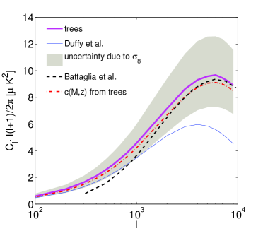
Figure 1: SZ power spectrum at $\nu=153$ GHz. Results shown are from the standard calculation (thin blue line), merger-tree calculation (thick pink line), a standard calculation with $c(M,z)$ fit to the merger-tree model (dot-dashed red line), adiabatic hydrodynamical simulations from Battaglia et al. (2010) (dashed black line). The grey area shows the uncertainty of the merger-tree calculation due to variations of $\sigma_{8}$.

The normalization of the power spectrum is known to be very sensitive to $\sigma_{8}$; we find the scaling $A_{SZ}\propto\sigma_{8}^{7.4}$, in accord with previous studies. The grey bands in Figure 1 correspond to $\sigma_{8}=0.8\pm 0.03$, a level of uncertainty determined from a joint analysis of WMAP7, BAO and SN data (Komatsu et al., 2011).

The fiducial model presented in Figure 1 results in an overall normalization well above the level obtained from the latest SPT measurement (Reichardt et al., 2011): $A_{SZ}(\ell=3000)=3.65\pm 0.69$ $\mu$K². Below we will show that within the uncertainties in the gas model, the gas mass fraction and the value of $\sigma_{8}$, our calculation is consistent with these measurements.

To compare the above results with those from simulations, we show in Figure 1 the power spectrum determined from an adiabatic hydrodynamical simulation by Battaglia et al. (2010) , rescaled to $\nu=153$ GHz. It is very interesting that both the normalization and the shape of the power spectrum obtained in our treatment agree well with the full numerical calculation, in spite of the very different approach used in the simulations. Battaglia et al. (2010) also calculated the power spectrum in the case when radiative cooling, star formation, supernova and AGN feedback were included, and found a reduction of power at small scales due to expansion of the gas to larger radii. Similar results were obtained by Shaw et al. (2009) and Sehgal et al. (2010), with different normalizations depending on the amount of energy feedback. While we have not attempted to model feedback mechanisms in this work, the agreement of our model with numerical calculations in the simple adiabatic case shows that our description of the hierarchical growth of clusters and the intrinsic scatter in their properties is reasonably realistic. We stress that even though we make several simplifying assumptions, including that of hydrostatic equilibrium, we still get a better agreement with simulations than in the standard approach. The modeling of IC gas can be further refined, as we discuss below.

There are two major differences between the merger-tree calculation and the standard treatment with the scaling relation from Duffy et al. (2008): the normalization in the former case is higher, and the peak shifts to higher multipoles ($\ell\sim 6000$ vs. $\ell\sim 4000$ in the latter case). These features can be understood in terms of the modified $c(M,z)$ relation that is deduced from the merger-tree algorithm. When we fit the average $c(M,z)$ relation from the merger-tree model to a general form $c=A(M/M_{pivot})^{B}(1+z)^{C}$ that is used by Duffy et al. (2008), we obtain $A=11.99^{+0.42}_{-0.43}$, $B=-0.079\pm 0.005$ and $C=-0.34\pm 0.03$ for $M_{pivot}=2\times 10^{12}h^{-1}M_{\odot}$, with $2\sigma$ confidence level (CL), but this function provides a poorer fit to our results than equation (14), whereas Duffy et al. (2008) obtain for their sample of relaxed halos $A=9.23^{+0.17}_{-0.16}$, $B=-0.09\pm 0.009$ and $C=-0.69\pm 0.05$ ($1\sigma$ CL). Thus, the merger-tree model predicts a slightly higher normalization of the $c(M,z)$ relation, which is partly responsible for the higher normalization of the SZ power spectrum, and a significantly lower redshift dependence, which also contributes to the increase in the power spectrum normalization and shifts the peak to higher multipoles (since clusters at higher redshifts are more concentrated and have a larger contribution to the SZ power). Indeed, when we calculate the SZ power spectrum with the scaling relation from Duffy et al. (2008), but with the redshift dependence parameter $C=-0.34$ taken from our merger-tree model, the peak shifts to $\ell\sim 5000$ and the normalization increases by $\sim 14\%$. An additional difference between the calculation performed with the $c(M,z)$ relation from equation (14) and the full merger-tree calculation, appears because the concentration parameter has an approximately log-normal distribution function: there are more halos with higher-than-average $c$ than with lower-than-average.

To what extent are these predictions for the concentration parameter reliable? There is some observational evidence that the concentration parameter is in fact higher than predicted by N-body simulations. For example, the concentration parameters measured by Schmidt & Allen (2007) from X-ray observations of $34$ dynamically relaxed clusters in the redshift range $z=0.06-0.7$ are significantly greater than those predicted by Duffy et al. (2008) for the same masses and redshifts. In a large dataset compiled by Comerford & Natarajan (2007), which consists of $62$ clusters at redshifts up to $z=0.89$ and masses up to at least $\sim 2\times 10^{15}M_{\odot}$, the normalization of the concentration parameter is found to be higher by at least $20\%$ than the results of numerical simulations. A similar conclusion is reached by Wojtak & Łokas (2010), who analyzed kinematic data of $41$ clusters at redshifts $z<0.1$. A recent X-ray analysis of $44$ clusters in the redshift range $0.1-0.3$ by Ettori et al. (2010) found a normalization of $c$ consistent with numerical simulations, although note that their constraint on the cosmological parameters produces a rather high $\sigma_{8}=1.0\pm 0.2$.

Interestingly, several strong lensing studies of massive clusters (e.g., Zitrin et al., 2011) found anomalously large Einstein radii and concentration parameters when compared with predictions from numerical simulations. The results of the merger-tree model suggest that perhaps these concentration parameters, although higher than the average values, are not incompatible with the $\Lambda$CDM model.

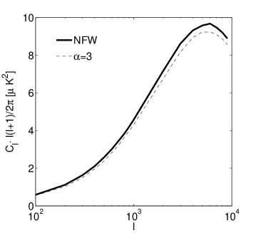
Figure 2: SZ power spectrum for different density profiles of DM halos. Shown are results for an NFW profile (solid line) and the profile in equation (15) with $\alpha=3$ (dashed line).

It is important to note that the simulations of Duffy et al. (2008) span the mass range of $10^{11}-10^{15}h^{-1}M_{\odot}$, similar to other numerical studies, while the masses that are important in the context of the SZ effect are $10^{13}-10^{16}h^{-1}M_{\odot}$. Low-mass and low-redshift halos outnumber high-mass halos by several orders of magnitude; the $c(M,z)$ relations are thus heavily weighted by the statistics of the low mass halos.

For example, the sample of Duffy et al. (2008) contains $1269$ sufficiently well-resolved halos at $z=0$, of which typically less than $\sim 0.1\%$ are above $10^{14}h^{-1}M_{\odot}$ if their relative abundance approximately follows the Sheth-Tormen MF. At $z=0.5$ only $\sim 0.03\%$ of all the halos are expected to have masses above $10^{14}h^{-1}M_{\odot}$. On the other hand, the parameters $B$ and $C$ are expected to vary with both mass and redshift (Gao et al., 2008; Muñoz-Cuartas et al., 2011; Prada et al., 2011). Indeed, when we fit the average merger-tree results only in the range $z=0-1$, $M=10^{13}-10^{14}h^{-1}M_{\odot}$ we obtain $B=-0.09$, $C=-0.46$, closer to the values in Duffy et al. (2008). This example demonstrates the inherent difficulty of numerical simulations to produce large samples of halos due to computational limitations. It is possible that because of the relatively small sample size numerical simulations overestimate the redshift evolution of the concentration parameter which biases the predicted SZ power spectrum.

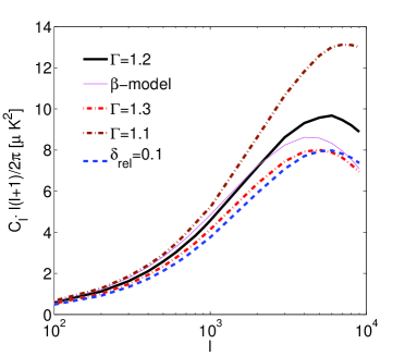
Figure 3: SZ power spectrum for different gas models: polytropic with different values of the adiabatic index, non-thermal pressure component, and $\beta$-model with $\beta=2/3$.

Our merger-tree approach enables us to test alternative DM halo density profiles, which is not possible in analytical calculations that are based on pre-calibrated scaling relations. As an example, we explore the following modification of the NFW profile:

$$\rho_{d}(r)=\frac{2^{\alpha}\rho_{s}}{r/r_{s}(1+r/r_{s})^{\alpha}}$$ (15)

for $\alpha>2$ (equations (3-5) are replaced by the appropriate solution for the new DM potential). Figure 2 shows that this modification with $\alpha=3$ has a minor effect on the amplitude of the power spectrum, as it affects only weakly the integrated gas pressure in the outer regions of clusters.

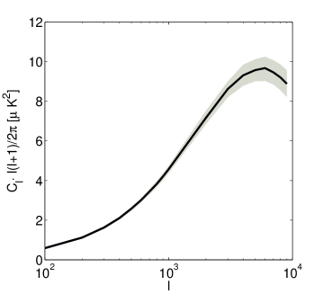
Figure 4: SZ power spectrum with merger-tree model parameters in the range $q=7-13$, $\kappa=4-6$ (grey area) and the fiducial model $q=10$, $\kappa=5$ (thick line).

All the calculations in this work were performed with the simple IC gas model described in Section 2. As was recently shown in several studies (Shaw et al., 2010; Trac, Bode & Ostriker, 2011; Efstathiou & Migliaccio, 2011), the strength of the SZ effect is very sensitive to the details of IC gas physics, for example a modest amount of non-thermal pressure can significantly lower the power spectrum. Here we explore the possibility of non-thermal pressure support, as well as slight variations in the parameters of the polytropic model. Figure 3 compares the results for different values of the adiabatic index $\Gamma$, a $\beta-$model and a polytropic model with a non-thermal pressure component. For simplicity we assume that the non-thermal component is a constant fraction of the total pressure:

$$P_{tot}=P_{thermal}+P_{rel}=(1+\delta_{rel})P_{thermal},$$ (16)

with $\delta_{rel}=0.1$ as a representative value.

It can be seen that the SZ power spectrum is very sensitive to slight changes in the value of the adiabatic index away from $\Gamma=1.2$, an average value deduced from numerical simulations. In accord with previous studies, we find that a small constant fraction of non-thermal pressure obviously reduces the normalization of the power spectrum but does not affect its shape.

Figure 4 shows the uncertainty in our calculation due to the merger-tree model parameters $q$, which is the maximal allowed ratio for major merger events, and $\kappa$, which describes the initial distance between two clusters that are about to merge. As expected, this uncertainty is smaller than $\sim 7\%$.

Our fiducial model assumes $f_{g}=0.1$, a constant gas mass fraction across the whole mass and redshift range. However, the fraction of hot gas in clusters varies with mass and redshift of observation. The mass dependence arises from various galactic processes including star formation, ram pressure stripping of gas from galaxies, and galactic winds. While the full redshift evolution of the gas mass fraction is not known, it clearly reflects aspects of cluster formation and evolution, which include also the effects of internal processes that re-distribute cluster baryons, those same processes that also imprint the (related) mass dependence. The latter was deduced in several X-ray studies of low redshift clusters (Vikhlinin et al., 2009; Giodini et al., 2009). Giodini et al. (2009) derived the following dependence based on a combined sample of $41$ clusters at $z\leq 0.2$ observed by Vikhlinin et al. (2006), Arnaud, Pointecouteau & Pratt (2007) and Sun et al. (2009):

$$f_{g}=(9.3\pm 0.2)\times 10^{-2}\left(\frac{M_{500}}{2\times 10^{14}M}_{\odot}\right)^{0.21\pm 0.03}\left(\frac{h}{0.7}\right)^{-1.5}.$$ (17)

We note that this fit is not valid beyond $M\simeq 10^{15}M_{\odot}$.

Not knowing the explicit scaling of the gas mass fraction with redshift, we can only account for its mass dependence by adopting the relation $f_{g}=M_{gas,500}/M_{tot,500}=M_{gas,virial}/M_{tot,virial}$. To avoid having a baryon fraction greater than the cosmic mean, which arises in high-mass clusters if the scaling relations above are strictly followed, we set an upper limit of $f_{cosmic}=\Omega_{b}/\Omega_{m}$.

The power spectrum, calculated with the gas mass fraction from equation (17) and assuming $\delta_{rel}=0.1$ is shown in Figure 5. It can be seen that our result is consistent with the SPT measurement if we allow for an uncertainty in $\sigma_{8}$ (Komatsu et al., 2011): $\sigma_{8}=0.8\pm 0.03$.

While we did not account for the possible redshift evolution of the gas mass fraction, we note that precise measurements of the SZ power spectrum may actually be used to deduce, or significantly constrain the redshift evolution of $f_{g}$, especially so when $\sigma_{8}$ is more precisely determined.

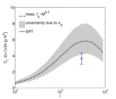
Figure 5: SZ power spectrum calculated with the gas mass fraction taken from equation (17) and $\delta_{rel}=0.1$. Blue dot with error bars represents the SPT measurement (Reichardt et al., 2011) at $\ell=3000$. The grey area shows the uncertainty due to variation in $\sigma_{8}$.

The expected cluster number counts are presented in Figure 6. We show the results of a standard calculation with $c(M,z)$ taken from Duffy et al. (2008) and from equation (14), as well as the merger-tree calculation repeated $10$ times so as to probe the distribution functions of the cluster properties. There is $\sim 15\%$ difference between the results of the merger-tree model and the standard calculation, a level of variance that could have appreciable ramifications on precise cosmological parameter extraction based on cluster number counts (Holder, Haiman & Mohr, 2001; Wang et al., 2004).

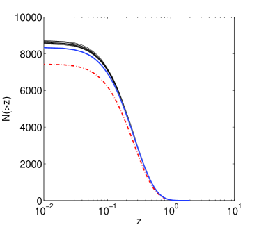
Figure 6: SZ cluster number counts above a specified redshift. Shown are results of a standard calculation with a $c(M,z)$ relation from Duffy et al. (2008) (red dot-dashed line), with $c(M,z)$ from a fit to the merger-tree model (blue solid line), and the full merger-tree calculation (black lines).

A major source of uncertainty in calculations of the SZ effect is the halo mass function. It is evident that the accuracy with which the MF can be determined in a given numerical simulation is reduced at higher redshifts, especially at the high mass end, due to the limited volume of the simulation. To illustrate this point, we can estimate the expected number of halos at different redshifts according to the Tinker MF in the simulations that were used to calibrate it. For example, for $z=1.25$ the number of halos per unit $\ln M$ is expected to be less than $\sim 100$ for $M>3\cdot 10^{14}M_{\odot}$, while at $z=2.5$ there is less than one halo with mass around $2\cdot 10^{14}M_{\odot}$ per unit $\ln M$ in the combined simulation volume.

It can be argued that large masses are rare at high redshifts and their contribution to the SZ power spectrum, although uncertain, is not important. Figure 7 shows the relative contribution of different masses and redshifts to the integral in equation (7) in the following way: we calculate this expression for $\ell=4000$ with different $z_{max}$ (x-axis) and $M_{max}$ (y-axis) and plot the result as a fraction of the fiducial value for which we took $z_{max}=2$ and $M_{max}=10^{16}h^{-1}M_{\odot}$. The contours are for constant fraction of the fiducial value. Two important features can be seen in Figure 7: (a) we have to integrate at least up to $z\sim 1.4$ to have a reliable estimate of the effect, and (b) masses above $2\cdot 10^{14}M_{\odot}$ contribute roughly $\sim 50\%$ of the effect (over the whole redshift range). It is clear that a large error in the MF even at $z\sim 1.25$ (which only worsens at higher redshifts) is very detrimental to the reliability of the calculation.

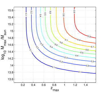
Figure 7: The value of the integral in equation (7) for various $z_{max}$ (x-axis) and $M_{max}$ (y-axis) relative to the fiducial values $z_{max}=2$ and $M_{max}=10^{16}h^{-1}M_{\odot}$, for $\ell=4000$. Contours show constant fractions of the fiducial value; the calculations were performed using the fitting formula in equation (14).

Finally, it should be emphasized that there is an inherent limitation in the accuracy of cluster MF deduced from dynamical cosmological simulations. This stems from the appreciable impact of baryonic processes (both stellar and gaseous) on cluster evolution. As an example we briefly mention here the conclusion of Stanek, Rudd & Evrard (2009) that number densities of clusters in their hydrodynamical simulations deviate by $10\%-60\%$ from those predicted by Tinker et al. (2008).

4 Discussion

We have presented a new analytical method of calculating the thermal SZ power spectrum and cluster number counts. This merger-tree method takes into account the intrinsic scatter in the halo parameters and their dependence on the redshifts of formation and observation that results from the hierarchical evolution of clusters. In particular, our model provides a good statistical description of the high-mass and high-redshift halos.

We have demonstrated that our approach, which does not rely on pre-calibrated scaling relations, allows to explore different density profiles of DM halos. In addition, since the cosmological parameters can be changed in each run of the merger-tree code and no scaling relations are inserted by hand, our approach is more suitable for cosmological parameter estimation studies than the standard analytic method.

We stress that the approach presented here differs from adding scatter in the various observable parameters to the standard analytic calculation, since in this case the scaling relations and the scatter itself are inserted by hand, whereas here they are intrinsic to the model and its predictions.

Our calculations predict a higher power spectrum normalization than the standard calculation which uses the $c(M,z)$ relation from Duffy et al. (2008) (for the same IC gas model), and a shift of the peak to higher multipoles. In addition, the merger-tree model predicts higher cluster number counts than the standard approach (again, for the same IC gas model). These differences can be explained by the modified $c(M,z)$ relation that is predicted by the merger-tree model. In particular, it has a higher normalization and a slower evolution with redshift than the results of Duffy et al. (2008). We argue that the higher normalization of the concentration parameter is more compatible with observations, while the faster redshift evolution of Duffy et al. (2008) results from the fact that their sample is heavily weighted by low-mass low-redshift halos, where the dependence on redshift is expected to be stronger. The excellent agreement between our results and the adiabatic hydrodynamical simulations by Battaglia et al. (2010) further support our conclusions.

As anticipated, we have found the SZ power spectrum is quite sensitive to the assumed IC gas model. Among the parameters that can strongly influence the SZ power are the gas mass fraction and the amount of non-thermal pressure and their variation with cluster mass and redshift. Our fiducial model, which assumes a constant $f_{g}=0.1$ produces a level of the SZ power spectrum significantly higher than recent measurements by the SPT. When we adopt a scaling of the gas mass fraction with mass $f_{g}\propto M^{0.2}$, inferred by Giodini et al. (2009), the (current) SPT measurement falls within the range of uncertainty in $\sigma_{8}$ which extends to lower power levels due to the mass-dependent gas fraction. Clearly, more detailed modeling of the gas mass fraction is needed for meaningful comparison with observations of the thermal SZ effect. Note also that we adopted a class of polytropic gas models; different models can be readily explored in the context of our merger-tree approach.

Another basic source of uncertainty is the halo MF. We have shown that the high-mass, high-redshift halos, for which the MF calibration is least certain, have a relatively large contribution to the SZ power spectrum. In this work we have used the Sheth-Tormen MF, but our approach can be extended to include other mass functions. This can be achieved by either calibrating the conditional MF that we use to build the merger trees to an up-to-date numerical simulation, in the spirit of Parkinson, Cole & Helly (2008), or constructing a theoretically motivated conditional MF that provides a better fit to simulations.

In the calculations presented here we assumed spherical symmetry for all halos. However, it is possible to extend our approach to account for halo triaxiality by modeling each halo in the tree as an ellipsoid either with constant values of the axis ratios, or with values drawn randomly from a probability distribution.

In this work we calculated the power spectrum of the SZ thermal component. Using our approach it is possible to calculate also the power due to the SZ kinematic component due to random cluster motions by assigning a peculiar velocity to each halo. This contribution is expected to be a small fraction of that from the thermal component. However, we cannot use our method to calculate the full kinematic power which also has contributions from matter outside of clusters. Therefore, our approach is better suited for calculations of cluster number counts and cosmological parameter estimation which relies on cluster counts, since they depend only on the signal that originates from matter within clusters.

The approach presented in this work provides a computationally efficient way to explore the uncertainties discussed above, and to gain an improved understanding of the influence of the evolution of galaxy clusters on their various observable properties.

References

- Allen, Evrard & Mantz (2011) Allen S. W., Evrard A. E., Mantz A. B., 2011, ARA&A, 49, 409
- Arnaud, Pointecouteau & Pratt (2007) Arnaud M., Pointecouteau E., Pratt G. W., 2007, A&A, 474, L37
- Battaglia et al. (2010) Battaglia N., Bond J. R., Pfrommer C., Sievers J. L., Sijacki D., 2010, ApJ, 725, 91
- Bonamente et al. (2008) Bonamente M., Joy M., LaRoque S. J., Carlstrom J. E., Nagai D., Marrone D. P., 2008, ApJ, 675, 106
- Bond et al. (2005) Bond J. R. et al., 2005, ApJ, 626, 12
- Comerford & Natarajan (2007) Comerford J. M., Natarajan P., 2007, MNRAS, 379, 190
- Duffy et al. (2008) Duffy A. R., Schaye J., Kay S. T., Dalla Vecchia C., 2008, MNRAS, 390, L64
- Dvorkin & Rephaeli (2011) Dvorkin I., Rephaeli Y., 2011, MNRAS, 412, 665
- Efstathiou & Migliaccio (2011) Efstathiou G., Migliaccio M., 2011, ArXiv e-prints
- Ettori et al. (2010) Ettori S., Gastaldello F., Leccardi A., Molendi S., Rossetti M., Buote D., Meneghetti M., 2010, A&A, 524, A68+
- Fowler et al. (2010) Fowler J. W. et al., 2010, ApJ, 722, 1148
- Gao et al. (2008) Gao L., Navarro J. F., Cole S., Frenk C. S., White S. D. M., Springel V., Jenkins A., Neto A. F., 2008, MNRAS, 387, 536
- Giodini et al. (2009) Giodini S. et al., 2009, ApJ, 703, 982
- Holder, Haiman & Mohr (2001) Holder G., Haiman Z., Mohr J. J., 2001, ApJ, 560, L111
- Holder, McCarthy & Babul (2007) Holder G. P., McCarthy I. G., Babul A., 2007, MNRAS, 382, 1697
- Komatsu & Seljak (2002) Komatsu E., Seljak U., 2002, MNRAS, 336, 1256
- Komatsu et al. (2011) Komatsu E. et al., 2011, ApJS, 192, 18
- Lacey & Cole (1993) Lacey C., Cole S., 1993, MNRAS, 262, 627
- Lueker et al. (2010) Lueker M. et al., 2010, ApJ, 719, 1045
- Monaco, Theuns & Taffoni (2002) Monaco P., Theuns T., Taffoni G., 2002, MNRAS, 331, 587
- Muñoz-Cuartas et al. (2011) Muñoz-Cuartas J. C., Macciò A. V., Gottlöber S., Dutton A. A., 2011, MNRAS, 411, 584
- Navarro, Frenk & White (1995) Navarro J. F., Frenk C. S., White S. D. M., 1995, MNRAS, 275, 720
- Ostriker, Bode & Babul (2005) Ostriker J. P., Bode P., Babul A., 2005, ApJ, 634, 964
- Parkinson, Cole & Helly (2008) Parkinson H., Cole S., Helly J., 2008, MNRAS, 383, 557
- Prada et al. (2011) Prada F., Klypin A. A., Cuesta A. J., Betancort-Rijo J. E., Primack J., 2011, ArXiv e-prints
- Reichardt et al. (2011) Reichardt C. L. et al., 2011, ArXiv e-prints
- Roncarelli et al. (2007) Roncarelli M., Moscardini L., Borgani S., Dolag K., 2007, MNRAS, 378, 1259
- Sadeh & Rephaeli (2004) Sadeh S., Rephaeli Y., 2004, New Astronomy, 9, 373
- Sadeh, Rephaeli & Silk (2007) Sadeh S., Rephaeli Y., Silk J., 2007, MNRAS, 380, 637
- Schäfer et al. (2006) Schäfer B. M., Pfrommer C., Bartelmann M., Springel V., Hernquist L., 2006, MNRAS, 370, 1309
- Schmidt & Allen (2007) Schmidt R. W., Allen S. W., 2007, MNRAS, 379, 209
- Sehgal et al. (2010) Sehgal N., Bode P., Das S., Hernandez-Monteagudo C., Huffenberger K., Lin Y.-T., Ostriker J. P., Trac H., 2010, ApJ, 709, 920
- Seljak, Burwell & Pen (2001) Seljak U., Burwell J., Pen U.-L., 2001, Phys. Rev. D, 63, 063001
- Shaw et al. (2010) Shaw L. D., Nagai D., Bhattacharya S., Lau E. T., 2010, ApJ, 725, 1452
- Shaw et al. (2009) Shaw L. D., Zahn O., Holder G. P., Doré O., 2009, ApJ, 702, 368
- Sheth & Tormen (1999) Sheth R. K., Tormen G., 1999, MNRAS, 308, 119
- Shimon, Sadeh & Rephaeli (2011) Shimon M., Sadeh S., Rephaeli Y., 2011, MNRAS, 412, 1895
- Shirokoff et al. (2011) Shirokoff E. et al., 2011, ApJ, 736, 61
- Springel, White & Hernquist (2001) Springel V., White M., Hernquist L., 2001, ApJ, 549, 681
- Springel et al. (2005) Springel V. et al., 2005, Nature, 435, 629
- Stanek, Rudd & Evrard (2009) Stanek R., Rudd D., Evrard A. E., 2009, MNRAS, 394, L11
- Sun et al. (2009) Sun M., Voit G. M., Donahue M., Jones C., Forman W., Vikhlinin A., 2009, ApJ, 693, 1142
- Tinker et al. (2008) Tinker J., Kravtsov A. V., Klypin A., Abazajian K., Warren M., Yepes G., Gottlöber S., Holz D. E., 2008, ApJ, 688, 709
- Trac, Bode & Ostriker (2011) Trac H., Bode P., Ostriker J. P., 2011, ApJ, 727, 94
- Vikhlinin et al. (2009) Vikhlinin A. et al., 2009, ApJ, 692, 1033
- Vikhlinin et al. (2006) Vikhlinin A., Kravtsov A., Forman W., Jones C., Markevitch M., Murray S. S., Van Speybroeck L., 2006, ApJ, 640, 691
- Wang et al. (2004) Wang S., Khoury J., Haiman Z., May M., 2004, Phys. Rev. D, 70, 123008
- Wojtak & Łokas (2010) Wojtak R., Łokas E. L., 2010, MNRAS, 408, 2442
- Zitrin et al. (2011) Zitrin A., Broadhurst T., Barkana R., Rephaeli Y., Benítez N., 2011, MNRAS, 410, 1939