Strongly star forming galaxies in the local Universe with nebular He II 4686 emission

Abstract

We present a sample of 2865 emission line galaxies with strong nebular ${\mathrm{He}}\,\textsc{ii}\>\lambda 4686$ emissions in Sloan Digital Sky Survey Data Release 7 and use this sample to investigate the origin of this line in star-forming galaxies. We show that star-forming galaxies and galaxies dominated by an active galactic nucleus form clearly separated branches in the ${\mathrm{He}}\,\textsc{ii}\>\lambda 4686/\mathrm{H}\beta$ versus $[{\mathrm{N}}\,\textsc{ii}]\>\lambda 6584/\mathrm{H}\alpha$ diagnostic diagram and derive an empirical classification scheme which separates the two classes. We also present an analysis of the physical properties of 189 star forming galaxies with strong ${\mathrm{He}}\,\textsc{ii}\>\lambda 4686$ emissions. These star-forming galaxies provide constraints on the hard ionizing continuum of massive stars. To make a quantitative comparison with observation we use photoionization models and examine how different stellar population models affect the predicted ${\mathrm{He}}\,\textsc{ii}\>\lambda 4686$ emission. We confirm previous findings that the models can predict ${\mathrm{He}}\,\textsc{ii}\>\lambda 4686$ emission only for instantaneous bursts of 20% solar metallicity or higher, and only for ages of $\sim 4-5$ Myr, the period when the extreme-ultraviolet continuum is dominated by emission from Wolf-Rayet stars. We find however that 83 of the star-forming galaxies (40%) in our sample do not have Wolf-Rayet features in their spectra despite showing strong nebular ${\mathrm{He}}\,\textsc{ii}\>\lambda 4686$ emission. We discuss possible reasons for this and possible mechanisms for the ${\mathrm{He}}\,\textsc{ii}\>\lambda 4686$ emission in these galaxies.

1 Introduction

The ionizing continuum of stars at $\lambda<912$ Å is of major importance for interpreting emission line observations of galaxies because many of the strong lines observed in the spectra of galaxies, such as $[{\mathrm{O}}\,\textsc{iii}]\>\lambda 5007$, $[{\mathrm{Ne}}\,\textsc{iii}]\>\lambda 3869$ and ${\mathrm{He}}\,\textsc{ii}\>\lambda 4686$, have ionization potentials in excess of 13.6 eV. Despite this importance we are severely limited by interstellar absorption in observing stellar spectra in this spectral window directly (e.g. Hoare et al., 1993). Although we can get direct information at slightly longer wavelengths with space-based UV spectroscopy (e.g. Crowther et al., 2002), most of our knowledge about the $\lambda<912$Å region is based on indirect evidence, even for solar metallicity.

A promising way to indirectly obtain information on the stellar ionizing continuum is to compare emission line properties (e.g. flux, equivalent width) to predictions from photoionization codes such as CLOUDY (Ferland et al., 1998) or MAPPINGS III (Allen et al., 2008). In practice these kinds of studies provide modest constraints on stellar atmosphere models (e.g. Crowther et al., 1999). However where predictions of models differ significantly, this approach can yield useful information. This is the approach we will adopt in this work, where we will make use of the ${\mathrm{He}}\,\textsc{ii}\>\lambda 4686$ nebular emission line to place constraints on stellar models and in particular on the ionization mechanism for this line.

The presence of a nebular ${\mathrm{He}}\,\textsc{ii}\>\lambda 4686$ line in the integrated spectrum of a galaxy indicates the existence of sources of hard ionizing radiation as the ionization energy for He⁺ is 54.4 eV ($\lambda\approx 228$ Å). This hard radiation can of course be produced by an active galactic nucleus (AGN), and most sources with luminous $\mathrm{He}$ ii  emission, in a flux limited sample, are indeed galaxies with an AGN. However the required hard radiation can also be provided by stellar sources and ${\mathrm{He}}\,\textsc{ii}\>\lambda 4686$ emission is frequently seen in $\mathrm{H}$ ii-galaxies. The line appears to be associated with young stellar populations; for instance, Bergeron et al. (1997) proposed Of stars as the sources of ${\mathrm{He}}\,\textsc{ii}\>\lambda 4686$ emission in dwarf galaxies. Subsequent discussion has mostly focused on Wolf-Rayet (WR) stars, although the distinction between these two classes is rather blurred (e.g. Gräfener et al., 2011). Schaerer (1996, see also ()) showed that the hard radiation field of WR stars could provide a good explanation of the nebular ${\mathrm{He}}\,\textsc{ii}\>\lambda 4686$ seen in $\mathrm{H}$ ii-galaxies. Guseva et al. (2000) tried to test this in a careful study of $\mathrm{H}$ ii-galaxies with prominent WR features. They were however unable to find WR features in 12 out of the 30 galaxies with nebular ${\mathrm{He}}\,\textsc{ii}\>\lambda 4686$ emission. The same lack of WR features in metal poor Blue Compact Dwarf (BCD) galaxies was pointed out by Thuan & Izotov (2005). They proposed that fast radiative shocks could be responsible for this emission (see also Garnett et al. 1991 ).

Similar results were reported by Brinchmann et al. (2008, hereafter B08), who analysed a sample of strong emission line galaxies in the Sloan Digital Sky Survey (SDSS, York et al., 2000) with ${\mathrm{He}}\,\textsc{ii}\>\lambda 4686$ emission. They showed that at least at metallicities of $12+\log\mathrm{O/H}>8$, there appeared to be a close correlation between WR features in galaxies and the presence of ${\mathrm{He}}\,\textsc{ii}\>\lambda 4686$ emission, but this appeared not to be so clear-cut at lower metallicities.

This apparent lack of connection of $\mathrm{He}$ ii  emission with the hard UV radiation from WR stars has also been seen in spatially resolved spectroscopic studies. Kehrig et. al (2008) performed an integral field spectroscopy study for the $\mathrm{H}$ ii galaxy II Zw 70 and found that the region associated with nebular ${\mathrm{He}}\,\textsc{ii}\>\lambda 4686$ emission was a few arcsec offset from the region with detected WR features. More recently Kehrig et. al (2011) and Neugent & Massey (2011) have presented studies of ${\mathrm{He}}\,\textsc{ii}\>\lambda 4686$ emission in M33. Both studies find some regions with nebular ${\mathrm{He}}\,\textsc{ii}\>\lambda 4686$ emission that are not associated with WR stars (see also Hadfield & Crowther 2007 , López-Sánchez & Esteban 2010 and Monreal-Ibero et al. 2010 ).

Thus a series of studies have shown that while ${\mathrm{He}}\,\textsc{ii}\>\lambda 4686$ emission frequently is found in association with WR stars, it appears not to be so in all cases, particularly at low metallicity. As mentioned above, possible additional sources of high energy photons could be X-ray binaries (Garnett et al. 1991, ), strong shocks (Dopita & Sutherland, 1996), low-level AGN activity and alternative models for stellar evolution (Yoon & Langer, 2005). However the existing studies do not show clear trends that allow us to distinguish between these scenarios.

Crucially the samples in most of the previous studies have not been selected specifically to study $\mathrm{He}$ ii  emission lines. To make progress in understanding this puzzle it is important to have as large as possible sample of $\mathrm{He}$ ii  emitting galaxies to allow one to study the relationship between $\mathrm{He}$ ii  emission and other physical properties. To this end we present here an analysis of emission line galaxies with strong ${\mathrm{He}}\,\textsc{ii}\>\lambda 4686$ emission in SDSS Data Release 7 (DR7, Abazajian et al., 2009).

In section 2 we discuss the sample selection and carefully account for AGN emission. The physical properties of the $\mathrm{He}$ ii  emitting galaxies are discussed in section 3 and the observed ${\mathrm{He}}\,\textsc{ii}\>\lambda 4686/\mathrm{H}\beta$ ratios are compared to model predictions in section 4. In section 5 we test these model predictions and investigate whether the presence of ${\mathrm{He}}\,\textsc{ii}\>\lambda 4686$ is associated with WR features. We find that low metallicity systems frequently do not show signs of WR stars. We discuss possible explanations for this finding in section 6 and conclude in section 7.

2 Data

Our sample is based on galaxy spectra from SDSS DR7 which cover a wavelength range of 3800-9200 Å. The spectra were analysed using the methodology discussed in Tremonti et al. 2004 (see also Brinchmann et al. 2004) to provide accurate continuum subtraction. All emission line sources were additionally analysed using the pipeline discussed in B08 to measure a wider gamut of emission lines. For each galaxy we measure 40 lines, These lines and the number of spectra that show these lines with $S/N>5.5$ are summarised in Table 1.

Measured line	Number of spectra	Fraction
$[{\mathrm{O}}\,\textsc{ii}]\>\lambda 3726,3729$	243977	16.51%
$[{\mathrm{Ne}}\,\textsc{iii}]\>\lambda 3869$	39143	2.65%
$\mathrm{H}{8}$	92230	6.24%
$[{\mathrm{Ne}}\,\textsc{iii}]\>\lambda 3967$	18367	1.24%
$\mathrm{H}\epsilon$	64120	4.34%
${\mathrm{He}}\,\textsc{i}\>\lambda 4026$	6368	0.43%
$[{\mathrm{S}}\,\textsc{ii}]\>\lambda 4069$	1503	0.10%
$\mathrm{H}\delta$	163534	11.07%
$\mathrm{H}\gamma$	295528	20.00%
$[{\mathrm{O}}\,\textsc{iii}]\>\lambda 4363$	7886	0.53%
${\mathrm{He}}\,\textsc{i}\>\lambda 4472$	15563	1.05%
$[{\mathrm{Fe}}\,\textsc{iii}]\>\lambda 4658$	2626	0.18%
${\mathrm{He}}\,\textsc{ii}\>\lambda 4685$	4034	0.27%
$[{\mathrm{Ar}}\,\textsc{iv}]\>\lambda 4711$	2893	0.20%
$[{\mathrm{Ar}}\,\textsc{iv}]\>\lambda 4740$	1074	0.07%
$\mathrm{H}\beta$	458324	31.02%
$[{\mathrm{O}}\,\textsc{iii}]\>\lambda 4959$	147734	10.00%
$[{\mathrm{O}}\,\textsc{iii}]\>\lambda 5007$	339212	22.96%
$[{\mathrm{N}}\,\textsc{i}]\>\lambda 5197$	1318	0.09%
$[{\mathrm{N}}\,\textsc{i}]\>\lambda 5200$	758	0.05%
$[{\mathrm{Cl}}\,\textsc{iii}]\>\lambda 5518$	160	0.01%
$[{\mathrm{Cl}}\,\textsc{iii}]\>\lambda 5538$	190	0.01%
$[{\mathrm{N}}\,\textsc{ii}]\>\lambda 5755$	4888	0.33%
${\mathrm{He}}\,\textsc{i}\>\lambda 5876$	75256	5.09%
$[{\mathrm{O}}\,\textsc{i}]\>\lambda 6300$	119328	8.08%
$[{\mathrm{S}}\,\textsc{iii}]\>\lambda 6312$	5552	0.38%
$[{\mathrm{O}}\,\textsc{i}]\>\lambda 6363$	16100	1.09%
$[{\mathrm{N}}\,\textsc{ii}]\>\lambda 6548$	361641	24.48%
$\mathrm{H}\alpha$	613338	41.51%
$[{\mathrm{N}}\,\textsc{ii}]\>\lambda 6584$	562659	38.08%
${\mathrm{He}}\,\textsc{i}\>\lambda 6678$	19084	1.29%
$[{\mathrm{S}}\,\textsc{ii}]\>\lambda 6717$	410903	27.81%
$[{\mathrm{S}}\,\textsc{ii}]\>\lambda 6731$	341386	23.11%
${\mathrm{He}}\,\textsc{i}\>\lambda 7065$	4232	0.29%
$[{\mathrm{Ar}}\,\textsc{iii}]\>\lambda 7135$	24034	1.63%
$[{\mathrm{O}}\,\textsc{ii}]\>\lambda 7318,19,29,30$	659	0.04%

Table 1: The table shows number of spectra that have the indicated line detected at $S/N>5.5$. The total number of analysed spectra is 1,477,411.

Our concern in this paper is not to analyse a volume- or magnitude-limited sample of galaxies, we therefore do not impose a redshift cut nor a magnitude limit. Since the blue wavelength cut-off of the SDSS spectrograph is $\sim 3800$Å, the $[{\mathrm{O}}\,\textsc{ii}]\>\lambda 3727,3729$ doublet falls outside the spectral range for $z<0.02$. This is a concern, because as we will see later 55% of our final sample fall in this region of redshift space and their oxygen abundances are therefore somewhat uncertain. When possible we use the $[{\mathrm{O}}\,\textsc{ii}]\>\lambda 7318-7330$ quadruplet instead (Kniazev et al., 2004), but as this is a fairly weak line and falls in a region with significant sky emission, we cannot always make use of this line.

2.1 Sample selection and classification

We select our sample requiring signal to noise ratio $>5.5$ in ${\mathrm{He}}\,\textsc{ii}\>\lambda 4686$, the resulting data set is given in Table LABEL:table5 . When the width of the $\mathrm{He}$ ii  line is consistent with that of the strong forbidden lines, we make the assumption that it has a nebular origin. Given that $\mathrm{He}$ ii  lines from individual WR stars typically are considerably broader than the forbidden lines in galaxies (e.g. B08), we feel this is a reasonable assumption. In addition we require a S/N$>3$ in each of $\mathrm{H}\beta$, $[{\mathrm{O}}\,\textsc{iii}]\>\lambda 5007$, $\mathrm{H}\alpha$ and $[{\mathrm{N}}\,\textsc{ii}]\>\lambda 6584$ emission lines to reliably classify our galaxies (Brinchmann et al. 2004, hereafter B04). The resulting sample contains 2865 spectra with strong nebular ${\mathrm{He}}\,\textsc{ii}\>\lambda 4686$ emission. In parallel, the spectra of the sample galaxies are examined for WR signatures using the approach discussed by B08. This resulted in a total sample of 385 spectra with likely and secure WR features (Class 1, 2 and 3 from B08). While we do not discuss the sample of all WR galaxies in DR7 with Class 1–3 in detail here, we note that it intersects that of the $\mathrm{He}$ ii  sample but is not a strict subset of it (see Table 3).

Figure 1 shows the redshift distribution for the fraction of the $\mathrm{He}$ ii  sample in the SDSS as a shaded grey histogram. The cut-off at $z\sim 0.4$ is due to $\mathrm{H}\alpha$ falling outside the spectrograph range. The red histogram shows the redshift distribution for the fraction of just the star-forming (SF) galaxies in the SDSS showing ${\mathrm{He}}\,\textsc{ii}\>\lambda 4686$ emission (see below for a discussion of the classification). For each class we have divided the number of $\mathrm{He}$ ii  emitting galaxies in that redshift bin by the number of similarly classified galaxies in the parent sample (SDSS galaxies that have S/N$>3$ in each of $\mathrm{H}\beta$, $[{\mathrm{O}}\,\textsc{iii}]\>\lambda 5007$, $\mathrm{H}\alpha$ and $[{\mathrm{N}}\,\textsc{ii}]\>\lambda 6584$) in that redshift bin. A constant value would therefore indicate a similar redshift distribution of the $\mathrm{He}$ ii  sample and the parent sample. It is clear from this that full $\mathrm{He}$ ii  sample closely follows the overall distribution of the SDSS, but that the star-forming galaxies with ${\mathrm{He}}\,\textsc{ii}\>\lambda 4686$ emission are predominantly found at low redshift. We can also see that less than 2% of all galaxies, and less than 1% of the star-forming galaxies in the SDSS DR7 show ${\mathrm{He}}\,\textsc{ii}\>\lambda 4686$ emission in their spectra.

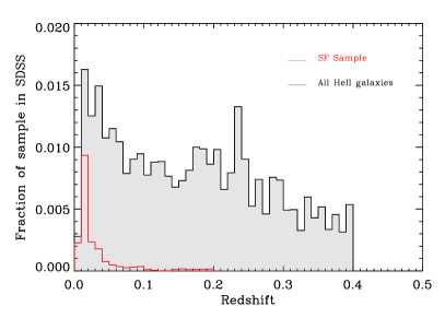
Figure 1: The redshift distribution of the full ${\mathrm{He}}\,\textsc{ii}\>$ sample, relative to that of the parent sample is shown as a shaded grey histogram. The red histogram shows the redshift distribution of the ${\mathrm{He}}\,\textsc{ii}\>$ SF sample relative to that of all star-forming galaxies in the parent sample; the parent sample consisting of those galaxies in the SDSS DR7 having $\mathrm{H}\beta$, $[{\mathrm{O}}\,\textsc{iii}]\>\lambda 5007$, $\mathrm{H}\alpha$ and $[{\mathrm{N}}\,\textsc{ii}]\>\lambda 6584$ detected at S/N$>3$. In comparison with the SDSS, it is clear that the galaxies in our SF sample have a redshift distribution strongly shifted toward low redshift.

To classify the dominant ionization source in each galaxy we follow previous studies in using the Baldwin et al. (1981, BPT) line ratio diagnostic diagram of $[{\mathrm{O}}\,\textsc{iii}]\>\lambda 5007/\mathrm{H}\beta$ versus $[{\mathrm{N}}\,\textsc{ii}]\>\lambda 6584/\mathrm{H}\alpha$ as our starting point (Figure 2). As has been discussed extensively (e.g. Terlevich et al., 1991; Kewley et al., 2001, hereafter Ke01; Kauffmann et al., 2003, hereafter Ka03; Kewley et al., 2006; Stasińska et al., 2006) this diagram allows a separation of AGN and star-forming galaxies because of their significantly different ionizing spectra, typically leading to high $[{\mathrm{O}}\,\textsc{iii}]\>\lambda 5007/\mathrm{H}\beta$ and $[{\mathrm{N}}\,\textsc{ii}]\>\lambda 6584/\mathrm{H}\alpha$ when an AGN is dominating the output of ionizing photons. Ke01 used a combination of stellar population synthesis and photoionization models to compute a theoretical maximum starburst line that isolates objects whose emission line ratios can be accounted for by photoionization by massive stars (below and to the left of the curve) from those where some other source of ionization is required. Ka03 defined an empirical upper limit to the $\mathrm{H}$ ii region sequence of SDSS galaxies in the BPT diagram. The region lying between these two lines represents objects more naturally explained as having a composite spectrum combining $\mathrm{H}$ ii region emission with a harder ionizing source. As we will see later, this interpretation is further corroborated by the ${\mathrm{He}}\,\textsc{ii}\>\lambda 4686/\mathrm{H}\beta$ ratios we find for our sample.

In the present study, we adopt a two-stage classification methodology. We start out by classifying all galaxies using the BPT diagram, and we will then refine our classifications for a subset of the galaxies using detailed inspection of the spectra and the ${\mathrm{He}}\,\textsc{ii}\>\lambda 4686$ line properties. For the initial classification we adopt a similar methodology to that of B04 and use the separation criteria defined by Ke01 and Ka03 to divide galaxies into different classes. Galaxies which are distributed above the Ke01 dividing line are considered AGNs, Galaxies between the Ke01 and Ka03 limits have composite classification, which means their source of ionizing radiation could be a combination of star formation and AGN activity. Finally, galaxies below the Ka03 line have a SF classification, which as we will see might be modified subsequently.

Figure 2 shows the BPT diagram for our sample, the Ke01 and Ka03 classification lines are shown as solid and dotted lines, respectively. The distribution of all emission line galaxies in the SDSS with $S/N>3$ in $\mathrm{H}\beta$, $[{\mathrm{O}}\,\textsc{iii}]\>\lambda 5007$, $\mathrm{H}\alpha$ and $[{\mathrm{N}}\,\textsc{ii}]\>\lambda 6584$ is shown as a grey-scale 2D distribution, where the grey-scale shows the logarithm of the number of galaxies in each bin. Blue circles show star-forming galaxies, triangles show composite galaxies and red squares mark AGNs. The grey dashed-dotted line shows the N2 (Pettini & Pagel 2004, , hereafter PP04) metallicity calibration for $\rm{12+\log O/H}=8.2$ ($[{\mathrm{N}}\,\textsc{ii}]\>\lambda 6584/\mathrm{H}\alpha=-1.2$). These classifications are the final ones and incorporate further information as described in the following.

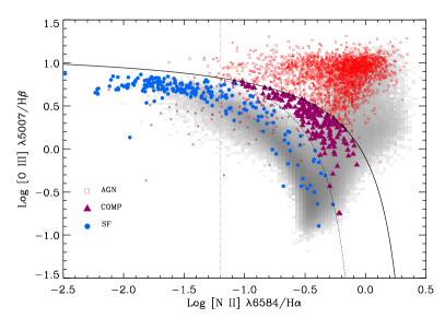
Figure 2: This plot shows the BPT diagnostic diagram for the sample. The Ka03 classification line is shown as a dotted line and Ke01 classification line as a solid line. The grey dashed-dotted line shows the N2 PP04 metallicity calibration for $\rm{12+\log O/H}=8.2$. The distribution of emission line galaxies in the SDSS is shown by the gray-scale 2D distribution where the grey-scale shows the logarithm of the number of galaxies in each bin. Blue circles show star-forming galaxies, triangles show composite galaxies and red squares mark AGNs. As discussed in the text, for some galaxies the classification has been adjusted which is why some objects in the star-forming region are classified as AGN. We mark these galaxies with a blue plus over the red square.

While the BPT diagram is a useful classification diagram, it is not particularly sensitive to low levels of AGN contamination and some progress can be made by including lines originating in the mostly neutral ISM (e.g. Kewley et al., 2006). For our purposes we however need to be very confident in the lack of AGNs in our sample and we will use the ${\mathrm{He}}\,\textsc{ii}\>\lambda 4686/\mathrm{H}\beta$ ratio for this purpose.

As remarked earlier, only photons with energy in excess of 54.4 eV can ionize He⁺ and thence produce the ${\mathrm{He}}\,\textsc{ii}\>\lambda 4686$ recombination line. If we consider single stellar population models from Starburst99 (Leitherer et al., 1999) at an age of 2 Myr (so that all stars are on the main sequence), we find that the integrated spectrum of this population typically contain 2-3 orders of magnitude fewer photons at this energy than at the energy required to ionize O⁺ (35.5 eV), which is needed to produce the $[{\mathrm{O}}\,\textsc{iii}]\>\lambda 5007$ line from collisionally excited O⁺². This line is therefore a very sensitive probe of AGN activity, particularly if used in conjunction with other line ratios. We therefore make use of the ${\mathrm{He}}\,\textsc{ii}\>\lambda 4686/\mathrm{H}\beta$ vs $[{\mathrm{N}}\,\textsc{ii}]\>\lambda 6584/\mathrm{H}\alpha$ diagram to further refine the classification of our sources. We show this diagram in Figure 3 where the symbols and colours are the same as in Figure 2.

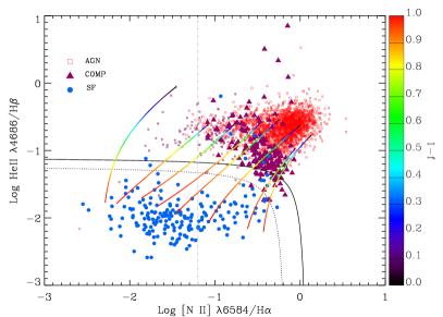
Figure 3: This plot shows our sample in the ${\mathrm{He}}\,\textsc{ii}\>\lambda 4686/\mathrm{H}\beta$ versus $[{\mathrm{N}}\,\textsc{ii}]\>\lambda 6584/\mathrm{H}\alpha$ diagnostic diagram. The dotted line shows an empirical line separating AGN and composite objects from star-forming galaxies. The grey dashed-dotted line shows the N2 PP04 metallicity calibration for $\rm{12+\log O/H}=8.2$. Symbols are the same as the BPT diagram. As ${\mathrm{He}}\,\textsc{ii}\>\lambda 4686$ have a higher ionization potential in comparison to $[{\mathrm{O}}\,\textsc{iii}]\>\lambda 5007$ and is much less sensitive to the electron temperature, we can clearly see separation between the classes in this diagram. The lines with colour gradients in the figure are simulated fluxes drawn from adding a random set of star-forming galaxy from the SDSS with emission line fluxes of a random set of AGN spectrum. The colouring of the lines corresponds to the fraction of the spectrum contributed by the star-forming galaxy, $1-f$, as indicated by the colour bar on the side. The solid line shows the theoretical upper limit for ${\mathrm{He}}\,\textsc{ii}\>\lambda 4686/\mathrm{H}\beta$ ratio.

Note that there is generally a very significant offset between the star-forming galaxies and AGNs in this diagram, in contrast to the gradual transition in much of the BPT diagram. To make a quantitative separation, we draw a random set of star-forming galaxies from the SDSS and gradually add their emission line fluxes to that of a random set of AGNs. We quantify this by the variable $f$ which is defined to be the fraction of the total $\mathrm{H}\beta$ flux comes from the AGN. The total flux is therefore $f\times AGN_{\textsc{Flux}}+(1-f)\times SF_{\textsc{Flux}}$. Changing $f$ will trace out a path in the diagnostic diagram in Figure 3 as illustrated by the lines with colour gradients in the figure. The colouring of the lines corresponds to $1-f$, as indicated by the colour bar on the side. We repeat this process for a thousand AGN and SF objects located in different bins in the $\mathrm{He}$ ii /$\mathrm{H}\beta$ diagram.

Based on this analysis we find that there is a well defined locus where 10% percent of the ${\mathrm{He}}\,\textsc{ii}\>\lambda 4686$ flux comes from an AGN (in this case $\approx 1$% of the $\mathrm{H}\beta$ flux comes from the AGN, see section 2.2 for further details). A good fit to this relation is given by:

$$\log(\frac{F_{{\mathrm{He}}\,\textsc{ii}\>\lambda{4686}}}{F_{\mathrm{H}\beta}})=-1.22+\frac{1}{8.92\log(\frac{F_{[{\mathrm{N}}\,\textsc{ii}]\>\lambda{6584}}}{F_{\mathrm{H}\alpha}})+1.32},$$ (1)

which is shown as a dotted line in Figure 3. The solid line shows a theoretical maximum starburst line, similar to the Ke01 line in the BPT diagram — we discuss this further below.

Finally, we look at the spectra of galaxies that we would classify as star-forming on the basis of their location in the BPT diagram, but that are offset from the rest of the star-forming galaxies in the $\mathrm{He}$ ii /$\mathrm{H}\beta$ diagram and check whether they show AGN features such as broad Balmer lines, strong $\mathrm{Ne\textsc{v}}\lambda 3426$, Fe ii emission or if they show a similar $[{\mathrm{O}}\,\textsc{iii}]\>\lambda 4363/\mathrm{H}\gamma$ ratio to that of AGNs. If some of these features are present, we change the classification from star-forming to AGN (these objects are plotted as red squares containing a blue cross in Figures  2 and 3). This happens for 127 (39%) galaxies. This is a conservative approach as we would exclude star-forming galaxies with strong outflows and hence a broad base to the Balmer lines for instance.

To estimate the maximum starburst line in Figure 3, we adopted the Charlot & Longhetti (2001, hereafter CL01) models. These combine evolving stellar populations models from Bruzual & Charlot (unpublished BC00 models using Padova 1994 tracks, see Bruzual & Charlot 2003 (BC03) for the current models) with the photoionization code Cloudy (Ferland et al., 1998) and adopt the simple dust attenuation prescription of Charlot & Fall (2000). The main model parameters for our calculations are the metallicity $Z$, the ionization parameter, $U$, the dust attenuation $\tau_{\mathrm{V}}$ and the dust-to-metal ratio, $\xi$, the model parameters used are given in Table 4, see B04 for a more detailed discussion. We use the CL01 Single Stellar Population (SSP) models since these achieve the highest possible ${\mathrm{He}}\,\textsc{ii}\>\lambda 4686/\mathrm{H}\beta$ values. We then identify the maximum ratio reached by the different models and use this upper envelope to define the maximum starburst line shown as a solid line in Figure 3.

Sample	He ii	He ii + WR
Total	2865	385
AGN	2474	234
Star forming	199	116
Composite	179	35

Table 3: An overall numerical summary of the $\mathrm{He}$ ii  sample. See section 2 for a summary of the selection and classification details. See section 5 for details on the WR classification.

This combination of classification methods means that there is not a one-to-one mapping between the location of an object in a diagnostic diagram and its final classification, as is clear from Figure 2 and 3. We also mention that we do not change classes for galaxies classified as AGNs or composites using the BPT diagram, but which fall within the star-forming region in the $\mathrm{He}$ ii /$\mathrm{H}\beta$ diagram and this is the reason why there are 7 AGN below our star-formation–AGN dividing line.

By contrasting Figure 2 and 3 we can make a couple of interesting observations. The first is that while in the BPT diagram we see a steady increase in $[{\mathrm{O}}\,\textsc{iii}]\>\lambda 5007/\mathrm{H}\beta$ with decreasing $[{\mathrm{N}}\,\textsc{ii}]\>\lambda 6584/\mathrm{H}\alpha$, in Figure 3 we see no major change in ${\mathrm{He}}\,\textsc{ii}\>\lambda 4686/\mathrm{H}\beta$ with $[{\mathrm{N}}\,\textsc{ii}]\>\lambda 6584/\mathrm{H}\alpha$. This indicates that ${\mathrm{He}}\,\textsc{ii}\>\lambda 4686/\mathrm{H}\beta$ and consequently the ionizing spectrum of stars at $\lambda<228$ Å vary only weakly with metallicity. The second difference between the two plots is that the ${\mathrm{He}}\,\textsc{ii}\>/\mathrm{H}\beta$ diagram can separate star-forming galaxies from composite galaxies better than BPT diagram since the ${\mathrm{He}}\,\textsc{ii}\>\lambda 4686/\mathrm{H}\beta$ ratio is more sensitive to the hardness of the ionizing source than $[{\mathrm{O}}\,\textsc{iii}]\>\lambda 5007/\mathrm{H}\beta$. We can use this to further support our supposition that the gas in the galaxies falling between the Ka03 and Ke01 lines in the BPT diagrams is ionized by a combination of stars and an AGN — while they are adjacent to the star-forming sequence in the BPT diagram they nearly all clearly separate from the star-forming sequence in the ${\mathrm{He}}\,\textsc{ii}\>$/$\mathrm{H}\beta$ diagram, corresponding to an AGN contribution to ${\mathrm{He}}\,\textsc{ii}\>\lambda 4686>50$%. Thus referring to these as composite objects appear to be justified.

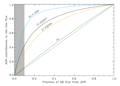
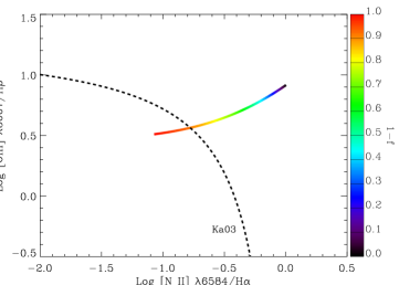
Figure 4: The upper panel shows the sensitivity of different lines to the presence of an AGN as a function of the fraction of the $\mathrm{H}\beta$ flux originating from an AGN. The grey shading indicates the region where a typical galaxy would be classified as star-forming in the BPT diagram (see text for details). We see that we might classify galaxies as star-forming even if 10% of the $\mathrm{H}\beta$ flux comes from AGN. The bottom panel illustrates the method used and shows the path traced by a galaxy in the BPT diagram as an increasing amount of AGN light is added to a star-forming galaxy spectrum. The colouring of the line corresponds to the fraction of the $\mathrm{H}\beta$ line flux contributed by the star-forming galaxy, $1-f$, as indicated by the colour bar on the side. The dashed line is the Ka03 classification line, the intersection of this line with the trajectory of the simulated flux is at $f\approx 0.1$.

2.2 AGN contamination estimation

In view of the clear separation of the AGN and star-formation branches in Figure 3, and our sensitivity to low-level AGN contamination, it is beneficial to study the impact of an AGN on the line ratios in more detail. This has been discussed in previous studies (e.g. B04, Stasińska et al. (2006)) but here we extend those efforts to include ${\mathrm{He}}\,\textsc{ii}\>\lambda 4686$.

We focus our attention on the BPT diagram as it is most widely used for emission line classification. We follow the same approach as in the previous section of adding gradually more of an AGN emission line spectrum with ${\mathrm{He}}\,\textsc{ii}\>\lambda 4686$ in emission at S/N$>3$, to a star-forming one, and find where it intersects the Ka03 line (see bottom panel of Figure 4). At this point the galaxy would cease to be classified as a star-forming galaxy. We repeat this for a total of 10,000 random combinations of spectra. The median AGN contribution to $\mathrm{H}\beta$ at the point where a galaxy ceases to be classified as star-forming is $\approx 10$%.

Figure 4 shows the region where a median galaxy would be classified as star-forming as the gray shaded region. On top of this we show the median trend for the fraction of flux in the indicated line as a function of the fraction of the $\mathrm{H}\beta$ flux coming from an AGN (shown for reference as the dashed diagonal line). We note that the exact shape and location of the $[{\mathrm{N}}\,\textsc{ii}]\>\lambda 6584$ and $[{\mathrm{O}}\,\textsc{iii}]\>\lambda 5007$ lines does depend somewhat on the AGN sample chosen but the qualitative trend remains the same.

What this figure shows, is firstly the well-known result that some lines are more sensitive to the presence of an AGN than others. As mentioned before, the Balmer lines are expected to have less than $10$% contribution from an AGN, while the $[{\mathrm{N}}\,\textsc{ii}]\>\lambda{6584}$ line can have more than 30% of its flux coming from an AGN, putting in question its use as an abundance indicator on its own (see also Stasińska et al. (2006)). But for our purposes, it is more important to note that by adopting a classification based on the BPT diagram, we would classify a galaxy as star-forming even when $\sim 65$% of its ${\mathrm{He}}\,\textsc{ii}\>\lambda 4686$ flux would come from an AGN.

We can now combine this with our previous result in Figure 3, where we found that only 10% of the ${\mathrm{He}}\,\textsc{ii}\>\lambda{4686}$ emission comes from an AGN in our refined star-forming sample. Applying this to Figure 4, we conclude that less than 1% of the $\mathrm{H}\beta$ flux comes from an AGN and the other lines will also only have very small contributions from an AGN implying we have a quite pure star-forming sample.

Our final sample of $\mathrm{He}$ ii  star-forming galaxies consists of 189 star-forming galaxies (199 spectra which have been summarised in Table LABEL:table4). As mentioned above we have also checked these spectra for the presence of WR signatures. We will return to a detailed discussion of this in section 5 but will use the result of this classification in the following plots.

Parameter	Range
$Z$, The metallicity	$-1<logZ/Z_{\odot}<0.6$, 24 steps
$U$, The ionization parameter	$-4.0<logU<-2.0$, 33 steps
$\tau_{V}$, The total dust attenuation	$0.01<\tau_{V}<4.0$, 24 steps
$\xi$, The dust-to-metal ratio	$0.1<\xi<0.5$, 9 steps

Table 4: The model grid used for the present work. We calculate this both for a constant star formation history at $t=10^{8}$ yrs as well as for an SSP.

3 Physical properties of the sample

While the majority of the galaxies in our sample have some physical parameters in the MPA-JHU value added catalogues, our galaxies are sufficiently extreme that we need to rederive some properties and add some physical parameters to what is in the MPA-JHU catalogue.

For the calculation of physical parameters we will adopt the Bayesian methodology outlined by Ka03 and B04. For each model we calculate the probability of that model given the data assuming Gaussian noise and obtain the Probability Distribution Function (PDF) of every parameter of interest by marginalisation over all other parameters (see Appendix A). We take the median value of each PDF to be the best estimate of a given parameter.

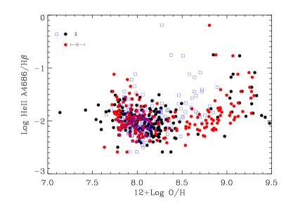
Figure 5: This plot shows ${\mathrm{He}}\,\textsc{ii}\>\lambda{4686}/\mathrm{H}\beta$ as a function of oxygen abundance (see text for details on the calculations). Oxygen abundances derived using the direct method are shown by black circles, we can not calculate oxygen abundances for 13 objects with this method as no $[{\mathrm{O}}\,\textsc{ii}]\>$ lines are available for them. Oxygen abundances derived from fits to the CL01 models are shown by red circles while the blue squares show the O3N2 oxygen abundance estimates. Note that the qualitative trends are similar, but the O3N2 estimator does not reach as high O/H values as the other two models. At low metallicity the three methods are in good agreement.

3.1 Mass measurements

The standard SDSS pipeline often segment nearby actively star-forming galaxies incorrectly, thus we need to redo the photometry of our galaxies. We do this using the Graphical Astronomy and Image Analysis Tools (GAIA). Most of our galaxies have strong emission lines within some of the broad-band filters. Prior to fitting we therefore correct the magnitudes for emission line contributions by assuming that the relative contribution of the lines found in the SDSS fiber spectra is applicable to the galaxy as a whole. As most galaxies in our sample appear to have a uniformly blue colour, presumably due to active star formation, we expect this to be a reasonable assumption.

Stellar masses are calculated as outlined above, by fitting a large grid of stochastic models to the SDSS u, g, r, i, z band photometry. The grid contains pre-calculated spectra for a set of 100,000 different star formation histories using the BC03 population synthesis models, following the precepts of (Gallazzi et al., 2005, 2008).

3.2 Emission line derived parameters

We use the CL01 model to analyse the emission lines in our sample. We adopt a constant star formation history (SFH) and use the same grid used by B04 (see Appendix A and B04 for further details). In total the model grid used for the fits have $2\times 10^{5}$ different models.

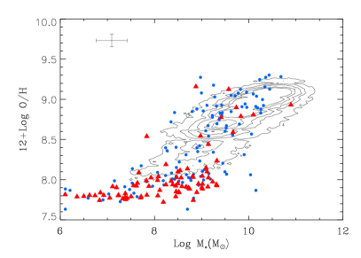
Figure 6: The contours show the mass-metallicity relation for SDSS galaxies (Tremonti et al. 2004, ). The present sample of star-forming galaxies with WR features is shown by blue circles, while the red triangles show the locations of those that do not show WR features. At low mass we see that our sample is offset from the rest bulk of the of SDSS but overall they sample much the same region.

The main quantity of interest for the present discussion is the oxygen abundance, quantified as $12+\log\rm{O/H}$. As there are significant differences between methods for estimating oxygen abundance (Kewley & Ellison, 2008), we have complemented the estimate from the CL01 method with two independent methods: Firstly, we estimate gas-phase oxygen abundances with the empirically calibrated estimators proposed by PP04. They used the line ratios of $[{\mathrm{O}}\,\textsc{iii}]\>\lambda 5007/\mathrm{H}\beta/[{\mathrm{N}}\,\textsc{ii}]\>\lambda 6584/\mathrm{H}\alpha$, the O3N2 method, and $[{\mathrm{N}}\,\textsc{ii}]\>\lambda 6584/\mathrm{H}\alpha$, the N2 method, as abundance indicators. For all objects with detected $[{\mathrm{O}}\,\textsc{iii}]\>\lambda 4363$ with $S/N>3$, we also use the $T_{e}$ method, or direct method, using the fitting formulae provided by Izotov et al. (2006) to estimate the oxygen abundances. For those objects without $[{\mathrm{O}}\,\textsc{iii}]\>\lambda 4363$, we adopt the electron temperature estimates from the CL01 models fits for the direct method calculation. Whenever we do not have $[{\mathrm{O}}\,\textsc{ii}]\>\lambda 3727,3729$, we use the $[{\mathrm{O}}\,\textsc{ii}]\>\lambda 7320,7330$ lines to calculate abundances. However, for 13 objects we are unable to use the direct method for estimating oxygen abundance as none of the $[{\mathrm{O}}\,\textsc{ii}]\>$ lines are available.

Figure 5 compares different abundance indicators in the ${\mathrm{He}}\,\textsc{ii}\>\lambda{4686}/\mathrm{H}\beta$ flux ratio versus oxygen abundance plane. The oxygen abundances derived using the direct method are shown by black circles while those derived from the fit to the CL01 model are shown by red circles, the blue squares show O3N2 oxygen abundances. The main conclusion we can draw from this comparison is that all methods agree well at low metallicity while at high metallicity the trends are similar but the O3N2 estimator reaches a lower maximum O/H. For concreteness we will adopt the CL01 estimates for the remainder of the paper but as our main focus will be on the low metallicity region, our results are robust to the estimator chosen.

Figure 6 shows the mass-metallicity relation for the sample compared to the mass-metallicity relation for all star-forming SDSS galaxies (Tremonti et al. 2004, ) shown as a contour. The sample galaxies with WR features in the spectra are shown as blue circles, while those that do not show WR features are plotted as red triangles, we will use the same symbols in the following. Overall there is a reasonable agreement with the main SDSS sample except for an offset towards slightly lower metallicity at a fixed mass at low masses.

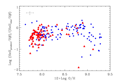
Figure 7: This figure shows the logarithm of the ratio of the model prediction for ${\mathrm{He}}\,\textsc{ii}\>\lambda 4686/\mathrm{H}\beta$ to the observed ratio as a function of oxygen abundance. Red triangles show the ratio for objects without WR features. It is clear that there is good agreement in the range $8.4<12+\log\mathrm{O/H}<8.8$, but at lower metallicity, the discrepancy between model and observations can be up to and order of magnitude. At higher than solar metallicity where an AGN contribution to the ${\mathrm{He}}\,\textsc{ii}\>\lambda 4686$ flux is more likely we see that model also fail to predict the same ratio as the observed value.

4 Model predictions

In the previous section we carried out an empirical analysis of the properties of star-forming galaxies in the SDSS which show strong nebular ${\mathrm{He}}\,\textsc{ii}\>\lambda 4686$ emission in their integrated spectra. Now we will build on the preceding to explore whether current stellar models can be used to explain the ${\mathrm{He}}\,\textsc{ii}\>\lambda 4686$ emission seen in the spectra of these galaxies. We start by predicting nebular ${\mathrm{He}}\,\textsc{ii}\>\lambda 4686$ emission for galaxies in our sample with the CL01 model. Then we change the stellar population model and explore the effect of changing the model on the predicted ${\mathrm{He}}\,\textsc{ii}\>\lambda 4686$ line flux.

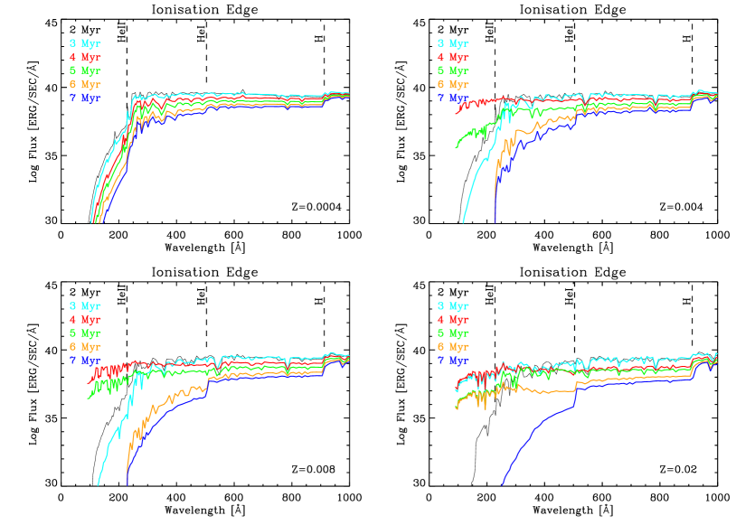
Figure 8: This figure shows the spectral energy distribution (SED) of an instantaneous burst calculated with Starburst99. Each panel corresponds to one metallicity and shows the SED for a range of ages as indicated. Note that the appearance of WR stars 4 Myr after the burst results in a much harder UV continuum. After 5-6 Myr the WR stars disappear and the UV continuum rapidly fades. Also note that in these models, the lowest metallicity SED does not show a significant WR phase.

4.1 CL01 predictions for nebular He II emission

We follow the same procedure as in the calculation of PDFs for the galaxy parameters in the previous section and calculate the likelihood of the model for each object in our sample by fitting the CL01 grid of models to the five important $\rm{[{\mathrm{O}}\,\textsc{ii}]\>\lambda 3727,3729}$, $\mathrm{H}\beta$, $[{\mathrm{O}}\,\textsc{iii}]\>\lambda 5007$, $\mathrm{H}\alpha$, $[{\mathrm{N}}\,\textsc{ii}]\>\lambda 6584$ emission lines.

We now want to see whether the models that reproduce the main strong lines in the optical spectrum also reproduce the ${\mathrm{He}}\,\textsc{ii}\>\lambda 4686$ emission line strength. We build the likelihood distribution of ${\mathrm{He}}\,\textsc{ii}\>\lambda 4686$ flux for each galaxy in the same way as before by weighting the ${\mathrm{He}}\,\textsc{ii}\>\lambda 4686$ flux in each model by the probability of that model. We take the median of the likelihood distribution as a prediction for nebular ${\mathrm{He}}\,\textsc{ii}\>\lambda 4686$ emission and the associated confidence interval to be the 16th-84th percentile range. We follow the same approach to estimate the ${\mathrm{He}}\,\textsc{ii}\>\lambda 4686/\mathrm{H}\beta$ ratio.

In Figure 7 we show the logarithm of the ratio of this model prediction for ${\mathrm{He}}\,\textsc{ii}\>\lambda 4686/\mathrm{H}\beta$ to the observed ${\mathrm{He}}\,\textsc{ii}\>\lambda 4686/\mathrm{H}\beta$ ratio as a function of oxygen abundance. It is clear that there is acceptable agreement between the model predictions and the observations in the range $8.4<12+\log\mathrm{O/H}<8.8$, but a model that can reproduce most the strong lines in the spectrum well, predicts up to one order of magnitude lower ${\mathrm{He}}\,\textsc{ii}\>\lambda 4686/\mathrm{H}\beta$ ratio than the observed value for some objects at lower metallicities. We also see a deviation at high metallicity — in this regime an AGN contribution to the $\mathrm{He}$ ii  line flux is more likely, both because the galaxies are more massive, and also because the star formation-AGN separation is more gradual in this regime. We will not discuss this mismatch further here.

The population synthesis model used in the CL01 models approximate the WR emission as black bodies at their effective temperature, note in passing that this is not the case in the current BC03 models. This will overestimate the hardness of the ionizing spectra compared to models that consider more sophisticated WR atmosphere models such as e.g. Starburst99 (Leitherer et al., 1999) and BPASS (Eldridge et al., 2008). Given the relatively simple treatment of the WR phases in the CL01 models, one might be concerned that the failure to match the data is due to an inherent weakness of the models. In the following we therefore look at the effect of different stellar evolution and atmosphere models on the prediction of ${\mathrm{He}}\,\textsc{ii}\>\lambda 4686$ emission line strengths.

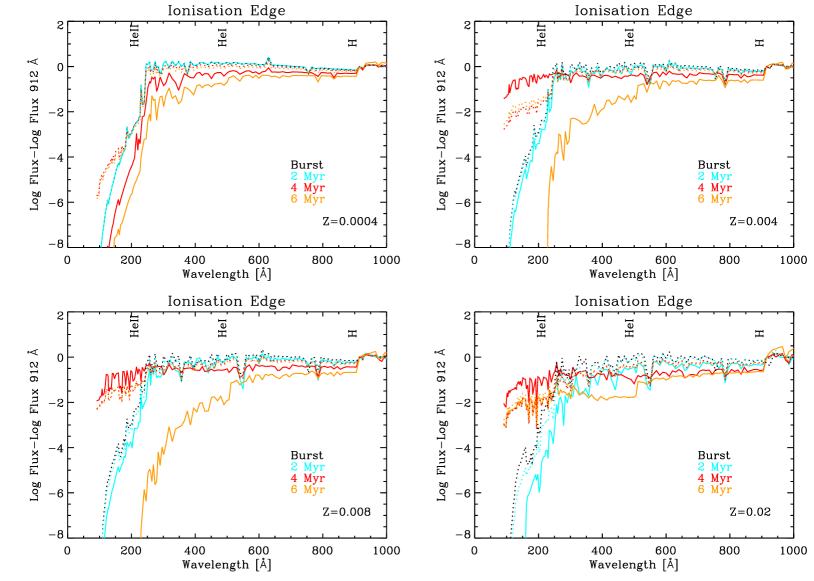
Figure 9: Each panel compare the calculated SED of two SFHs with starburst99 for a different metallicity, solid lines show SEDs of instantaneous burst and dotted lines show SEDs with constant star formation rate and different colours show different burst ages. Fluxes have been normalised to the flux at 912 Å. We can see although models with constant star formation form WR stars continuously after 4 Myr, the overall shape of the UV continuum is softer than in the instantaneous burst models because the continuous formation of luminous O stars softens the extreme UV spectrum for a fixed rate of hydrogen ionizing photons.

4.2 Starburst99 predictions

To better understand the origin of the ${\mathrm{He}}\,\textsc{ii}\>\lambda{4686}$ emission and its dependence on the stellar models adopted, we use the latest version (6.0) of the spectral synthesis code Starburst99 (Stb99, Leitherer et al., 1999, 2010) to calculate spectral energy distributions (SEDs) predictions for a range of ages and metal abundances. We calculate models with an instantaneous burst and a constant star formation history with a Kroupa IMF. We have explored a range of stellar evolution models but the differences are small so we only show the results of one model. For this we adopt the Padova AGB evolutionary tracks combined with Pauldrach/Hillier atmospheres (Smith et al. 2002, ), Stb99 uses O star model spectra from Pauldrach et al. (2001) and WR model spectra from the code of Hillier & Miller (1998). The models include stellar and nebular continuum. We create models with different metallicities (0.0004, 0.004, 0.008, 0.02, 0.05), where the reference solar metallicity is $Z_{\odot}=0.02$ An (Anders & Grevesse 1989). We do not consider dust and run the models up to 100 Myr with time-steps of $10^{5}$ years. Figure 8 shows the resulting SEDs for an instantaneous burst with a range of metallicities. Each panel corresponds to one metallicity as indicated and shows the time of the SED for six burst ages. The plots show clearly that the appearance of WR stars, 4 Myr after the burst, results in a harder UV continuum shortwards of the He⁺ ionizing edge at 228 Å. After $\sim 5$ Myr the WR stars disappear and the UV continuum becomes softer. This is in good agreement with the discussion in Schaerer & Vacca (1998, see their Figure 9), which is natural as those models lie at core of the WR modeling in Stb99. Figure 9 compares the SEDs of an instantaneous burst (solid line) with that of a continuous star formation model (dotted line). The SEDs have been normalised at 912Å, so have the same amount of hydrogen ionizing photons. The continuous star formation models form WR stars continuously after 3 Myr, but the overall shape of the UV continuum is softer than for instantaneous burst models because of the continuous formation of luminous O stars which dilute the SED for a given total mass.

To calculate the emission lines, we use the UV continuum generated by the Stb99 models as an input to the photoionization code Cloudy (version c08, Ferland et al., 1998). For each time step, ionization bounded models are calculated by varying the ionization parameter $\mathrm{\log U}=$ $-2$, $-3$, $-4$, where for consistency with the CL01 models we calculate the ionization parameter at the edge of the Strömgren sphere, and a constant hydrogen density of $\log\rm{n_{H}/cm^{-3}}=2.5$. This range in ionization parameter spans the range found by (1996) in their analysis of intensely star-forming galaxies (approximately $-3.5<\log\mathrm{U}<-2.5$). Figure 10 shows the calculated ${\mathrm{He}}\,\textsc{ii}\>\lambda 4686/\mathrm{H}\beta$ ratio versus $[{\mathrm{N}}\,\textsc{ii}]\>\lambda 6584/\mathrm{H}\alpha$ for different metallicities and different ionization parameters in the left panel and different burst ages in the right panel. The triangles along each model line correspond to the metallicities (0.02, 0.2, 0.4, 1) $Z_{\odot}$ in the left panel and to ages of 3, 4, 5, and 6 Myr in the right panel. In the left panel we fix the the age to 4 Myr, and in the right we set $\log\mathrm{U}=-2$. The galaxies in our sample are shown as filled purple circles. From these plots we can see how the ${\mathrm{He}}\,\textsc{ii}\>\lambda 4686/\mathrm{H}\beta$ ratio depends on age, metallicity and ionization parameter. The lowest metallicity considered in this work is $Z=0.02$ $Z_{\odot}$ and for this metallicity there is a strong discrepancy between the model predictions and the observed data but predictions for other metallicities at 4 Myr agree well with the observed ${\mathrm{He}}\,\textsc{ii}\>\lambda 4686/\mathrm{H}\beta$ ratios.

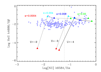
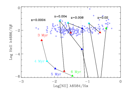
Figure 10: The left panel shows the starburst99 instantaneous burst model prediction for the ${\mathrm{He}}\,\textsc{ii}\>\lambda 4686/\mathrm{H}\beta$ ratio for different ionization parameters at a fixed age of 4 Myr. The triangles along each line correspond to the metallicities (0.02, 0.2, 0.4, 1) $Z_{\odot}$ and our sample galaxies are shown as purple circles. The right hand panel shows the same for a range of different metallicities and ages with $\log\mathrm{U}$ set to $-2$. The triangles along each model line correspond to the burst ages (3, 4, 5, 6) Myr. Note that the lowest metallicity model is unable to cover the observational data. The grey dashed-dotted lines in each panel show the N2 PP04 metallicity calibration for $\rm{12+\log O/H}=8.2$

The models can predict the ${\mathrm{He}}\,\textsc{ii}\>\lambda 4686$ emission line ratio, but only for instantaneous bursts with metallicity of 20% solar and above, and only for ages of $\sim 4-5$ Myr, the period when the extreme-ultraviolet continuum is dominated by emission from WR stars. For burst ages younger than 4 Myr and older than 6 Myr, and for models with a continuous star formation (not shown here), the softer ionizing continuum results in an emission spectrum that has too weak $\mathrm{He}$ ii  lines to be consistent with the observational data.

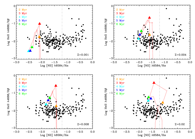
Figure 11: The plots show the prediction of instantaneous burst binary model (BPASS code) for ${\mathrm{He}}\,\textsc{ii}\>\lambda 4686/\mathrm{H}\beta$ ratio for different metallicities (0.05, 0.2, 0.4,1) $z_{\odot}$ and burst ages. The grey dashed-dotted line shows the N2 PP04 metallicity calibration for $\rm{12+\log O/H}=8.2$.

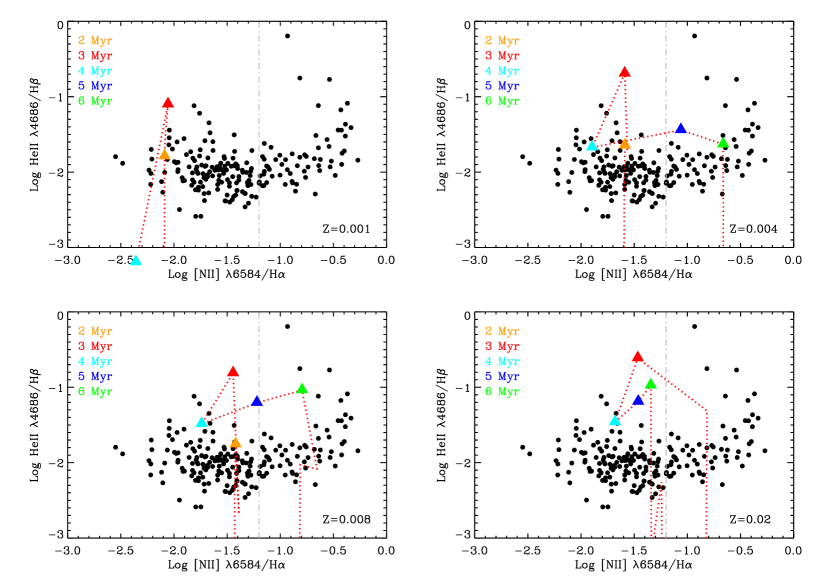
Figure 12: The plots show the prediction of instantaneous burst single-star model using the BPASS code for the ${\mathrm{He}}\,\textsc{ii}\>\lambda 4686/\mathrm{H}\beta$ ratio for different metallicities, (0.05, 0.2, 0.4, 1) $Z_{\odot}$, and burst ages. The grey dashed-dotted line shows the N2 PP04 metallicity calibration for $\rm{12+\log O/H}=8.2$.

4.3 The effect of binary evolution on the He II 4686 emission

The Stb99 models consider single-star evolution only, but it is well-known that massive stars are frequently found in binaries and higher order systems which can have a major effect on the evolution of massive stars. To explore this possibility we compare the observed ${\mathrm{He}}\,\textsc{ii}\>\lambda 4686/\mathrm{H}\beta$ ratio to the prediction of the Binary Population and Spectral Synthesis (BPASS, Eldridge et al 2008, 2009, 2011) model. The BPASS code includes a careful treatment of the effect of binary evolution on massive short lived stars, and Eldridge et al found that including massive binary evolution in the stellar population leads to WR stars forming over a wider range of ages up to 10 Myr which increases the UV flux at later times. In Figure 11 and Figure 12 we show the observed ${\mathrm{He}}\,\textsc{ii}\>\lambda 4686/\mathrm{H}\beta$ ratio in comparison with their instantaneous burst binary and single-star population models, respectively. Each panel shows four different metallicities (0.05, 0.2, 0.4,1) $Z_{\odot}$. The grey dashed-dotted line shows the N2 PP04 metallicity calibration for $\rm{12+\log O/H}=8.2$. We should note that the lowest metallicity in these plots is a factor of 2.5 higher than that of Stb99 (0.02 $Z_{\odot}$).

We get the highest value for the ${\mathrm{He}}\,\textsc{ii}\>\lambda 4686/\mathrm{H}\beta$ ratio at 3 Myr and the period with elevated ${\mathrm{He}}\,\textsc{ii}\>\lambda 4686/\mathrm{H}\beta$ lasts longer. Comparing Figure 11 and Figure 12, there is not a striking difference in the predicted peak ratio for ${\mathrm{He}}\,\textsc{ii}\>\lambda 4686/\mathrm{H}\beta$ between single-star and binary population models but clearly the binary model predict an elevated ratio for a longer period of time than the single-star models.

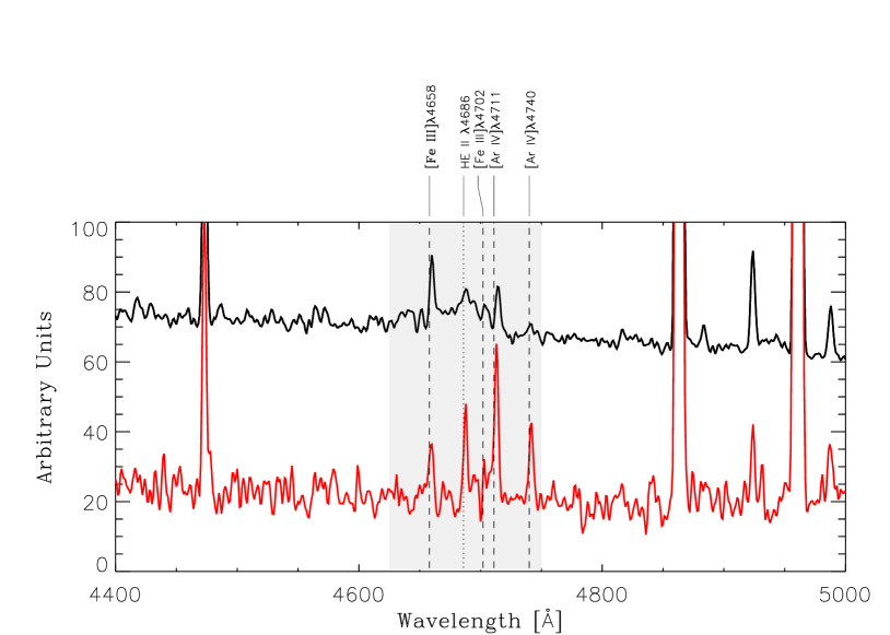
Figure 13: This plot shows a comparison between two stacked spectra of galaxies with $\mathrm{He}$ ii  emission. The black spectrum shows the result of stacking the spectra of all galaxies in our sample that show WR features. In this case we can clearly see the blue WR bump (gray shaded region). The red spectrum shows the result of stacking the spectra of all galaxies that show no WR features. Despite the increase in S/N we see no sign of WR features, strengthening our claim that this class of galaxies show no signs of WR features.

5 The origin of nebular He II 4686 emission

The preceding discussion makes it clear that in standard models for stellar evolution, only during the phases where the ionizing spectrum is dominated by WR stars will we see strong ${\mathrm{He}}\,\textsc{ii}\>\lambda 4686$ emission. This was already pointed out by Schaerer (1996) and our results are in good agreement with that work as well as a number of other previous works (Schaerer & Vacca, 1998; Guseva et al., 2000; Thuan & Izotov, 2005).

What has been less studied is the direct test of this prediction, namely to ask whether WR features are seen whenever ${\mathrm{He}}\,\textsc{ii}\>\lambda 4686$ is observed. Kehrig et. al (2011) and Neugent & Massey (2011) have recently studied individual star forming regions with ${\mathrm{He}}\,\textsc{ii}\>\lambda 4686$ emission in the Local Group and have shown that while most $\mathrm{He}$ ii -emitting regions also show evidence of WR stars, not all do. In more distant galaxies, previous efforts have primarily looked at $\mathrm{He}$ ii  emission in samples selected for other purposes. As an example, B08 looked at $\mathrm{He}$ ii  galaxies in SDSS DR6 and studied whether they showed WR features, but their sample selection was not optimised for finding galaxies with ${\mathrm{He}}\,\textsc{ii}\>\lambda 4686$ emission. The excellent analysis of Thuan & Izotov (2005) is another example, where the focus was on BCD galaxies. Since the present sample is selected purely on the presence of ${\mathrm{He}}\,\textsc{ii}\>\lambda 4686$, we can carry out this study with more reliability but we need to check for WR features in the spectra of our galaxies.

The presence of WR stars can be recognised via the WR bumps around $\lambda 4650$ Å(blue bump) and $\lambda 5808$ Å(red bump). The former is a blend of ${\mathrm{He}}\,\textsc{ii}\>\lambda 4686$ and several metal lines while the latter is caused by $\mathrm{C\textsc{iv}}\lambda 5801-12$ (see Crowther ARA&A review (2007), B08 and references therein). We have therefore inspected the spectra in our star-forming sample following the methodology described in B08 (see Table 3). Each spectrum is assigned a classification of 0 (no WR), 1 (possible WR), 2 (very probable WR), or 3 (certain WR). We will consider any spectrum with class 1, 2 or 3 to show WR features. To check the reliability of these classifications we can check whether duplicate observations of the same object are given the same classification. There are four sets of duplicate observations (0417-51821-513 Class 2, 0418-51817-302 Class 3, 0418-51884-319 Class 2), (0455-51909-073 Class 0, 0456-51910-306 Class 0), (0266-51602-089 Class 1, 0266-51630-100 Class 0) and (0308-51662-081 Class 3, 0920-52411-575 Class 3). Only for 0266-51602-089 and 0266-51630-100 is there uncertainty whether spectrum show evidence of WR features or not — we choose to keep the original classifications. This is in agreement with, but somewhat better than what we find for the full sample of WR galaxies from the B08 sample where the RMS classification uncertainty from duplicates is 0.4 classes without any apparent dependence on the median S/N of the spectra down to S/N$\sim 10$; at lower S/N we do not have sufficient numbers of duplicate observations to make a statement. In total we find that 116 of objects show WR features.

To check whether the non-detection of WR features is due to a low S/N, we have created stacked spectra of galaxies with and without WR features. The result of this exercise is shown in in Figure 13. The black line is the stack of spectra that show WR features while in red we show the stack of non-WR galaxies. We see no sign of WR features in the stack, further supporting the notion that this class of objects show no signs of WR features.

We now turn to explore whether there are physical differences in the galaxies showing WR features or not. Figure 14 shows the ratio of ${\mathrm{He}}\,\textsc{ii}\>\lambda 4686/\mathrm{H}\beta$ versus oxygen abundance for galaxies with (blue circles) and without WR features (triangles). The symbols for the non-WR galaxies, here and in the following, are coloured red for $12+\log\mathrm{O/H}<8.2$, and orange otherwise. At oxygen abundances lower than 8.2 we see there is a trend of increasing ${\mathrm{He}}\,\textsc{ii}\>\lambda 4686/\mathrm{H}\beta$ ratio towards lower metallicities. We interpret this as being due to a harder ionizing continuum at lower metallicities (e.g. Thuan & Izotov, 2005, and references therein). We also see a trend of increasing ${\mathrm{He}}\,\textsc{ii}\>\lambda 4686/\mathrm{H}\beta$ towards higher metallicity for $12+\log\mathrm{O/H}>8.7$. It is less clear what causes this, but since these are more massive systems with higher star formation rates and with stronger stellar winds due to their higher metallicity, it is likely that what we are seeing is due to an increased contribution of shocks and/or a low-level AGN contamination.

Another striking result is that for $12+\log\mathrm{O/H}>8.2$, essentially all $\mathrm{He}$ ii -emitting galaxies show WR features, in agreement with what one would expect from the models discussed in the previous section. At high metallicity there appear to be some systems that show a high ${\mathrm{He}}\,\textsc{ii}\>\lambda 4686/\mathrm{H}\beta$ ratios but no sign of WR stars. Since these are more massive systems, and fall intermediate between the SF and AGN groups in the ${\mathrm{He}}\,\textsc{ii}\>\lambda 4686/\mathrm{H}\beta$ versus $[{\mathrm{N}}\,\textsc{ii}]\>\lambda 6584/\mathrm{H}\alpha$ diagram, we interpret this as a likely sign of a low-level AGN contribution.

In Figure 15 we show the fraction of galaxies that show WR features as a function of metallicity. To calculate this we draw a number of random realisations of the data using the uncertainty estimates on the oxygen abundance to draw a random realisation. We also draw a random realisation of the WR classification assuming a random uncertainty in the classification of 0.4 as determined from the analysis of duplicate spectra as discussed above. We carry out 101 random realisations for each of the 101 bootstrap repetitions and calculate the median fraction of galaxies showing WR features in each metallicity bin as well as the 16%–84% scatter around the median which is shown by the error bars in Figure 15. What is clear is that there is a transition at around an oxygen abundance of $12+\log\mathrm{O/H}\approx 8.2\pm 0.1$. The uncertainty of $0.1$ dex encapsulates the fact that the exact value of this transition abundance depends somewhat on the metallicity calibration adopted and 0.1 dex corresponds to the scatter found when using the different calibrations discussed earlier.

As we showed in earlier, e.g. Figure 10, the ${\mathrm{He}}\,\textsc{ii}\>\lambda 4686/\mathrm{H}\beta$ ratio depends strongly on the age of the starbursts so it is reasonable to ask whether the systems without WR features are systematically younger or older than the systems that show WR features. In Figure 16 we test this by plotting the ${\mathrm{He}}\,\textsc{ii}\>\lambda 4686/\mathrm{H}\beta$ ratio versus $\mathrm{EW(\mathrm{H}\beta)}$ for the sample, where we take the $\mathrm{EW(\mathrm{H}\beta)}$ as a proxy for starburst age. We show galaxies with WR features by black and blue circles at high and low metallicities, respectively. Galaxies without WR features are as before shown by orange and red triangles at high and low metallicities. We see the ${\mathrm{He}}\,\textsc{ii}\>\lambda 4686/\mathrm{H}\beta$ ratios decrease with $\mathrm{EW(\mathrm{H}\beta)}$ for both WR and non-WR objects. However, galaxies without WR features show higher ratios than galaxies with WR feature for the same $\mathrm{EW(\mathrm{H}\beta)}$, especially at lower $\mathrm{EW(\mathrm{H}\beta)}$. Alternatively one might say that at a fixed ${\mathrm{He}}\,\textsc{ii}\>\lambda 4686/\mathrm{H}\beta$ the systems without WR features have a higher $\mathrm{EW(\mathrm{H}\beta)}$, or with our assumption, a younger starburst. It is not possible with our data to disentangle these two possibilities.

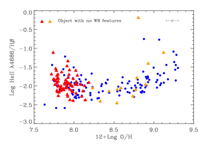
Figure 14: The ${\mathrm{He}}\,\textsc{ii}\>\lambda 4686/\mathrm{H}\beta$ ratio versus oxygen abundance for the sample. The blue solid circles show the location of galaxies with WR features. Galaxies which do not show WR features are indicated by red and orange triangles at lower and higher oxygen abundances than $12+\log\rm{O/H}=8.2$, respectively.

Figure 15: The fraction of objects with detected WR features in the $\mathrm{He}$ ii  sample as a function of gas-phase oxygen abundance. The points show the median fraction in each abundance bin and the error bars the 16%-84% scatter around the median (see text for details). While essentially all high-metallicity star-forming galaxies with ${\mathrm{He}}\,\textsc{ii}\>\lambda 4686$ nebular emission show WR features, this fraction drops rapidly at metallicities below $12+\log\rm{O/H}\approx 8.2$.

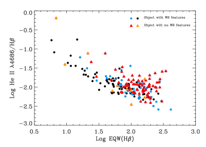
Figure 16: This plot shows the dependence of the ${\mathrm{He}}\,\textsc{ii}\>\lambda 4686/\mathrm{H}\beta$ ratio on the $\mathrm{EW(\mathrm{H}\beta)}$ and metallicity. We show galaxies with WR features by black and blue circles at high and low metallicities, respectively. Galaxies without WR feature are shown by orange and red triangles at high and low metallicities. We see the ${\mathrm{He}}\,\textsc{ii}\>\lambda 4686/\mathrm{H}\beta$ ratios decrease with $\mathrm{EW(\mathrm{H}\beta)}$ for both WR and non-WR objects. However, galaxies without WR features show higher ratios than galaxies with WR feature for the same $\mathrm{EW(\mathrm{H}\beta)}$, especially at lower $\mathrm{EW(\mathrm{H}\beta)}$s, alternatively one could read this to say that they have a high $\mathrm{EW(\mathrm{H}\beta)}$ (young age) for a given ${\mathrm{He}}\,\textsc{ii}\>\lambda 4686/\mathrm{H}\beta$ ratio.

6 Why are there galaxies with He II 4686 emission but no WR features?

The models that we discussed previously agree that WR stars are the source of the hard ionizing photons necessary to produce the ${\mathrm{He}}\,\textsc{ii}\>\lambda 4686$ emission. It is therefore a puzzle why some of the galaxies with nebular ${\mathrm{He}}\,\textsc{ii}\>\lambda 4686$ emission do not show stellar WR features. This lack of WR features has been pointed out before (e.g Thuan & Izotov, 2005), but this is the first time a clear trend with metallicity appears. In this section we therefore turn to discuss some possible reasons for this lack of WR features.

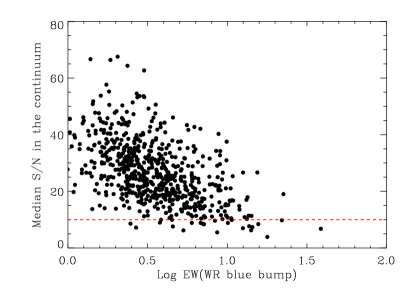
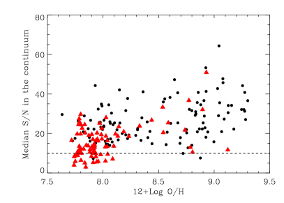
Figure 17: Top panel: The relationship between the equivalent width of the WR blue bump and the median S/N in the continuum for WR galaxies in SDSS DR7. We see that a S/N of 10 is sufficient to detect even very weak features. Bottom panel: The distribution of the median S/N in the continuum for WR and non-WR objects in the sample versus their oxygen abundance, we see that 20 out of 70 of the non-WR galaxies at $12+\log\mathrm{O/H}<8.2$ have S/N less than 10. See text for more discussion.

1. Differences in the $\mathbf{S/N}$ of the spectra
To detect the WR features we need fairly high S/N in the continuum as they are broad and weak features. In the top panel in Figure 17 we show the relationship between the equivalent width of the WR blue bump and the median S/N in the continuum for WR galaxies in SDSS DR7. We see that a S/N of 10 is sufficient to detect even very weak features. The distribution of the S/N for WR and non-WR objects in the sample versus their metallicities in the bottom panel shows that 20 out of 70 of the non-WR galaxies at $12+\log\mathrm{O/H}<8.2$ have S/N less than 10. Since the total number of galaxies at $12+\log\mathrm{O/H}<8.2$ is 115, if all the 20 low S/N galaxies are assumed to have WR features this brings the fraction of galaxies with WR features in this metallicity range from 30% to 43%. Thus low S/N could cause us to underestimate the WR fraction by at most $\sim 15$%. But the fact that the co-added spectrum in Figure 13 which has a higher S/N shows no WR features is suggestive that S/N might not be the problem for non-detection of WR features.

Furthermore even adding 15% would still mean that less than half $\mathrm{He}$ ii  emitters at low metallicity would show WR features. We also studied the difference in WR classification of duplicate observations as a function S/N and as remarked earlier, we saw no trend with S/N for more uncertain classification down to a S/N of 10. The dataset is insufficient to test this at lower S/N. Thus our conclusion is that it is unlikely that the systematic absence of WR features in low metallicity objects is due to low S/N in the spectra.

2. Weak lined WN stars
One possible reason for the lack of WR features in the most metal poor galaxies, is that the WR lines are too weak to be seen. It is well known (e.g. Conti et al., 1989; Crowther & Hadfield, 2006) that WR stars in the SMC have narrower and less luminous lines than equivalent stars in the Milky Way. Crowther & Hadfield (2006), for instance, find that He II lines in WR stars in the SMC are typically a factor of 4-5 weaker than the Milky Way and hence one would expect that in galaxies at the same distance, it would be harder to see WR features in lower metallicity systems. This is however countered by the fact that low metallicity systems on average are closer, and hence the SDSS fibre subtends a smaller physical size. Since WR emitting regions typically are small, they do not fill the 3” aperture in more distant galaxies, which means that the contrast of the WR features is being enhanced in low redshift systems. This is reflected in the fact that in the WR survey by B08, the equivalent width of the WR features in low metallicity systems (12 + Log O/H $<8.25$) is slightly higher than that in metal rich objects (12 + Log O/H $>8.5$), a mean of 5.1 Å vs 4.1 Å. Thus the increased contrast appears to approximately cancel out the decrease in line luminosity leading to a fairly constant detection potential with redshift. Thus we do not believe that this is the cause of the dearth of WR features in the low metallicity $\mathrm{He}$ ii  emitting galaxies, at least down to $12+\log\mathrm{O/H}\sim 8$. At very low metallicities, $12+\log\mathrm{O/H}\sim 7.5$, Eldridge & Stanway (2009) found that in their models the WR features become very weak and if those results are correct it should be extremely hard to detect WR features in those galaxies. We do however caution that I Zw 18 has very prominent WR features (e.g. Legrand et al., 1997), so at least some extremely metal poor galaxies do show clear WR features. Furthermore, even if we are unable to detect WR features at the very lowest metallicities, the same models predict strong WR features at $12+\log\mathrm{O/H}>8$, thus this is not a sufficient explanation for the result in Figure 15.
3. Shocks
Thuan & Izotov (2005) studied the hard ionizing radiation in very metal poor BCD galaxies in the local Universe and concluded that fast radiative shocks could be responsible for the nebular ${\mathrm{He}}\,\textsc{ii}\>\lambda 4686$ emission. Therefore, another possibility is that there is a contribution to the ${\mathrm{He}}\,\textsc{ii}\>\lambda 4686$ from shocks in the ISM (Dopita & Sutherland, 1996). That ${\mathrm{He}}\,\textsc{ii}\>\lambda 4686$ can have some contribution from shocks is plausible, but whether it can explain the systematic lack of WR features at low metallicity is less clear.

One question is whether shock models can reproduce the line luminosity in $\mathrm{He}$ ii  at low metallicities. Using the predictions of the Dopita et al. (2005) and Allen et al. (2008) shock models for the ${\mathrm{He}}\,\textsc{ii}\>\lambda 4686/\mathrm{H}\beta$ ratio versus $[{\mathrm{N}}\,\textsc{ii}]\>\lambda 6584/\mathrm{H}\alpha$, we found that we can only obtain a ratio comparable to the observed one for objects at high metallicity. A second issue centers on the observation that shocks would most likely come from supernovae and stellar winds, but the latter are though to be weaker at low metallicities. Shocks can also be induced by outflows from starbursts (e.g. galactic winds) and mergers but only two galaxies in our sample are interacting and show a perturbed morphology and we see no clear difference between the low- and high-metallicity subsamples.
4. X-ray binaries
Another candidate source for $\mathrm{He}$ ii  ionization that has been discussed in previous studies of ${\mathrm{He}}\,\textsc{ii}\>\lambda 4686$ emitting nebulae are massive X-ray binaries (Garnett et al. 1991, ). While these are likely present in many active star forming regions, the question here is why massive X-ray binaries should be more common at low metallicity. If the He⁺ ionizing photons at low metallicities come from X-ray binaries, we would expect an increasing binary fraction with decreasing metallicity. Without a theoretical justification for this, we consider an increased abundance of X-ray binaries at low metallicity to be an unlikely explanation for the trend seen in Figure 15.
5. post-AGB stars
Binette et al. (1994) demonstrated that photoionization by post-AGB stars can produce nebular ${\mathrm{He}}\,\textsc{ii}\>\lambda 4686$ emission. After about a few $10^{7}$ years (i.e, after massive stars disappear), the ionizing radiation comes from post-AGB stars. So, the ionization from post-AGB stars become more important in more evolved systems and this is not the case for our objects especially not for objects at low metallicities (c.f. Figure 16).

6. Spatial offset
One possible explanation for non detection of WR features is that there could be a significant spatial separation between the WR stars and the region emitting $\mathrm{He}$ ii . Kehrig et. al (2008) saw indeed such a spatial separation based on integral field spectra of II Zw 70. The found that the location of the WR stars and the ${\mathrm{He}}\,\textsc{ii}\>\lambda 4686$ emission appear to be separated by $\sim 80$pc.
Similarly, Izotov et al. (2006b) studied two-dimensional spectra of an extremely metal-deficient BCD galaxy SBS 0335-052E and showed that the ${\mathrm{He}}\,\textsc{ii}\>\lambda 4686$ emission line was also offset from the near evolved star clusters but in their case, by studying the kinematical properties of the ionized gas from the different emission lines they suggested that the hard ionizing radiation responsible for the ${\mathrm{He}}\,\textsc{ii}\>\lambda 4686$ emission was not related to the most massive youngest stars, but rather was related to fast radiative shocks.

If this offset between the WR stars and the region emitting $\mathrm{He}$ ii  might be an explanation for our non-detections of WR features, it would mean that such a spatial separation is much more common at low metallicity which is rather surprising, since stellar winds are thought to be considerably weaker there, however low metallicity galaxies are also on average closer so the SDSS fibre subtends a smaller physical scale so a smaller volume would need to be blown out by the wind (see Figure 18). To get a more quantitative estimate we calculate the gravitational binding energy of a cloud with radius 1.5” (SDSS aperture radius) at the redshift of each non-WR object. We assume a hydrogen density of $\sim$ 50 $cm^{-3}$. The median energy require to excavate a hole of this size, is of the order of $10^{55}$ erg for our full sample. For the lowest redshift objects the energy requirement is a much more manageable $10^{49}$ erg and thus in these cases the absence of WR features in the spectrum could be due to a spatial offset from the $\mathrm{He}$ ii  emitting region. At higher redshift the energetics makes this a much less likely explanation. The possibility does however warrant further examination and to test this we are undertaking a spectroscopic follow-up of a subsample of these sources.
7. Chemically homogeneous stellar evolution
A final explanation could be that the stellar populations at very low metallicities can have much higher temperatures than is currently expected in models. This would be the case if some stars rotated fast enough to evolve homogeneously (Maeder, 1987; Meynet & Maeder, 2007; Yoon & Langer, 2005; Yoon et al., 2006; Cantiello et al., 2007). In that case we can get a higher continuum at 228 Å and correspondingly a higher ${\mathrm{He}}\,\textsc{ii}\>\lambda{4686}/\mathrm{H}\beta$ ratio in comparison with non-homogeneous stellar evolution models. An appealing aspect of this, speculative, explanation is that homogeneous evolution is predicted to be more common at low metallicity. There are however currently no studies of the nebular ${\mathrm{He}}\,\textsc{ii}\>\lambda 4686$ line in the literature. Eldridge & Stanway (2011b) looked at the effect of quasi-homogeneous evolution in their binary models and showed that including it led to strengthened WR features at low redshift, in contrast to what we need. However that still leaves the possibility open that there is a period where strong nebular ${\mathrm{He}}\,\textsc{ii}\>\lambda 4686$ is seen but no WR features as that has not yet been tested.

7 CONCLUSION

We have presented a sample of rare star-forming galaxies with strong nebular ${\mathrm{He}}\,\textsc{ii}\>\lambda 4686$ emission spanning a wide range in metallicity. We have derived physical parameters for these galaxies and showed that emission line models that can reproduce the strong lines in the galaxy spectra are not able to predict the observed ratio of ${\mathrm{He}}\,\textsc{ii}\>\lambda 4686/\mathrm{H}\beta$ at low metallicities. In agreement with previous studies we found that current models for single massive stars are able to reproduce the ${\mathrm{He}}\,\textsc{ii}\>\lambda 4686/\mathrm{H}\beta$ ratio in galaxies in our sample, but only for instantaneous bursts of 20% solar metallicity or higher, and only for ages of $\sim 4-5$ Myr, the period when the extreme-ultraviolet continuum is dominated by emission from WR stars. For stars younger than 4 Myr or older than 5 Myr, and for models with a constant star-formation rate, the softer ionizing continuum results in ${\mathrm{He}}\,\textsc{ii}\>\lambda 4686/\mathrm{H}\beta$ ratios typically too low to explain our data. Including massive binary evolution in the stellar population analysis leads to WR stars occurring over a wider range in age which leads to acceptable agreement with the data at all metallicities sampled as long as WR stars are present.

However, the most notable result of our studies is that a large fraction of the galaxies in our sample do not show WR features and this fraction increases systematically with decreasing metallicity. We find that 70% of galaxies at oxygen abundances lower than 8.2 do not show WR features in their spectra. We discussed a range of different mechanism responsible for producing ${\mathrm{He}}\,\textsc{ii}\>\lambda 4686$ line apart from WR stars in these galaxies and conclude that spatial separation between WR stars and the region emitting $\mathrm{He}$ ii  emission can be a possible explanation for non-detection of WR features in these galaxies. Moreover, if the stellar population models at very low metallicities can have much higher temperatures than is currently expected in models, as would for instance be the case if some stars rotate fast enough to evolve homogeneously, then such models might explain the origin of the ${\mathrm{He}}\,\textsc{ii}\>\lambda 4686$ line and also the metallicity trend of the $\mathrm{He}$ ii  sample better. We will explore these possibilities in a future paper.

Appendix A Fitting models to the emission lines

The CL01 model grid is calculated by varying the model parameters, $U$, ionization parameter at the edge of the Strömgren sphere, $\tau_{V}$, total $V$–band optical depth, $\xi$, the dust-to-metal ratio of ionized gas, $\mu$, the fraction of the total optical depth in the neutral ISM contributed by the ambient ISM, and $Z$, the metallicity, over a certain range for 221 unequally spaced time steps from $t=0$ to $t=20Gyr$ (see Table 4).
In this paper we use the interpolated model grid of various luminosities for 50 time-steps from B04. This includes a total of $2\times 10^{5}$ different models. To fit to the data we adopt the Bayesian methodology described by Ka03. We obtain the PDF of every parameter of interest by marginalisation over all other parameters. The resulting PDF is used to estimate confidence intervals for each estimated physical parameter. We need to fit to at least five strong emission lines, $[{\mathrm{O}}\,\textsc{ii}]\>\lambda 3727,3729$, $\mathrm{H}\beta$, $[{\mathrm{O}}\,\textsc{iii}]\>\lambda 5007$, $\mathrm{H}\alpha$, $[{\mathrm{N}}\,\textsc{ii}]\>\lambda 6584$ to get a good constraint on the parameters. We take the median value of each parameter to be the best estimate of a given parameter.

In Figure 19 we illustrate our technique by showing the effect of adding lines on the PDFs of parameters when we fit a model to the data. We start with $[{\mathrm{O}}\,\textsc{ii}]\>\lambda 3727,3729$ and show how we get more well defined PDFs for the indicated parameters as we add the emission lines indicated on the left. We show the PDFs for dust attenuation parameter in $V$ -band, gas phase oxygen abundance, ionization parameter, dust-to-metal ratio of ionized gas and the conversion factor from $\mathrm{H}\alpha$ and [$\mathrm{O}$ ii]  luminosity to star formation rate (see CL01 for further details), for one object in our sample. The dust-to-metal ratio, $\xi$, is hard to constrain, except at high metallicity.

Figure 19: We show how the PDFs for dust attenuation parameter in $V$-band, gas phase oxygen abundance, ionization parameter of ionized gas, dust-to-metal ratio and $\mathrm{H}\alpha$ and [$\mathrm{O}$ ii]  efficiency factors change when we add more emission lines to the fit. $\xi$ is hard to constrain, except at high metallicity.

Table 2: The positions and the identifications of galaxies with nebular ${\mathrm{He}}\,\textsc{ii}\>\lambda 4686$ emission. OKSN is for galaxies having $SN>3$ in their $[{\mathrm{O}}\,\textsc{iii}]\>\lambda 5007$, $\mathrm{H}\beta$, $[{\mathrm{N}}\,\textsc{ii}]\>\lambda 6584$ and $\mathrm{H}\alpha$ lines. See B04 for the BPT classification. The full table is available in electronic form in http://www.strw.leidenuniv.nl/$\sim$shirazi/SB011/.

$\alpha(J2000)$	$\delta$	Plate–MJD–FiberID	$\log{\mathrm{He}}\,\textsc{ii}\>/\mathrm{H}\beta$	$\log[{\mathrm{N}}\,\textsc{ii}]\>/\mathrm{H}\alpha$	Class	Class(BPT)	SN	WR Features	Class(WR)
+11 59 09.71	+00 00 06.78	0285-51930-485	-0.93	-0.14	AGN	AGN	OKSN	Non-WR	—
+15 30 26.32	+00 00 10.81	0363-51989-400	-0.79	-0.31	AGN	AGN	OKSN	Non-WR	—
+08 58 28.60	+00 01 24.49	0470-51929-309	-0.84	-0.01	AGN	AGN	OKSN	WR	1
+13 06 00.68	+00 01 25.06	0294-51986-438	-1.12	-0.07	AGN	AGN	OKSN	Non-WR	0
+01 10 06.09	+00 01 33.00	0694-52209-113	-0.88	-0.36	AGN	AGN	OKSN	Non-WR	—

Table 5: The positions and identifications of the sample of star-forming galaxies with nebular ${\mathrm{He}}\,\textsc{ii}\>\lambda 4686$ emission.

Plate–MJD–FiberID	Z	$\alpha(J2000)$	$\delta$	ID	$\log{\mathrm{He}}\,\textsc{ii}\>/\mathrm{H}\beta$	$\log[{\mathrm{N}}\,\textsc{ii}]\>/\mathrm{H}\alpha$	$12+\log\rm{O/H}$	Features	Class	Other Names
0752-52251-340	0.00291	+00 09 53.09	+15 44 04.80	51	-1.35	-1.67	7.92$\pm$0.09	Non-WR	0	N/A
0390-51900-291	0.09437	+00 17 28.29	-00 56 24.98	13	-1.57	-0.56	9.27$\pm$0.05	WR	2	N/A
0390-51900-445	0.09840	+00 21 01.03	+00 52 48.08	14	-1.96	-1.10	8.83$\pm$0.04	WR	2	UM 228
0753-52233-094	0.01424	+00 24 25.95	+14 04 10.65	52	-1.98	-1.36	8.10$\pm$0.12	WR	3	N/A
0418-51884-319	0.01791	+00 32 18.59	+15 00 14.17	19	-1.97	-1.52	8.01$\pm$0.07	WR	2	SHOC 022
0691-52199-389	0.19554	+00 42 52.31	+00 27 30.09	48	-0.75	-0.82	8.88$\pm$0.05	WR	2	N/A
1905-53706-628	0.15928	+00 49 13.88	+00 24 01.99	138	-1.64	-2.05	7.85$\pm$0.06	Non-WR	0	N/A
0394-51913-075	0.16742	+00 55 27.46	-00 21 48.77	15	-1.76	-0.89	8.90$\pm$0.04	WR	2	N/A
0695-52202-137	0.00556	+01 15 33.82	-00 51 31.17	49	-2.32	-1.27	8.31$\pm$0.35	WR	3	NGC 0450
2329-53725-536	0.00975	+01 25 34.19	+07 59 24.40	169	-2.02	-2.22	7.80$\pm$0.04	Non-WR	0	N/A
0429-51820-495	0.05662	+01 47 07.04	+13 56 29.29	20	-1.95	-1.52	8.02$\pm$0.05	Non-WR	0	N/A
0666-52149-331	0.15155	+01 59 53.07	-08 13 48.99	44	-1.73	-1.43	8.04$\pm$0.06	Non-WR	0	SHOC 099
1073-52649-409	0.03994	+02 13 06.62	+00 56 12.44	73	-1.97	-1.58	8.09$\pm$0.05	Non-WR	0	UM 411
0667-52163-634	0.00492	+02 15 13.98	-08 46 24.39	45	-1.12	-1.81	7.74$\pm$0.09	Non-WR	0	SHOC 111
0456-51910-306	0.08222	+02 40 52.20	-08 28 27.43	24	-1.60	-1.63	8.02$\pm$0.04	Non-WR	0	SHOC 133
1070-52591-072	0.00421	+02 42 39.86	-00 00 58.64	72	-1.41	-0.33	8.93$\pm$0.25	Non-WR	0	M077
0456-51910-076	0.00456	+02 48 15.94	-08 17 16.51	23	-2.11	-1.90	7.87$\pm$0.08	Non-WR	0	N/A
1666-52991-310	0.03992	+03 14 31.71	+41 05 25.95	117	-1.95	-1.40	8.08$\pm$0.19	WR	1	N/A
0413-51821-480	0.06868	+03 17 43.12	+00 19 36.84	16	-0.77	-0.54	9.07$\pm$0.11	WR	2	N/A
1733-53047-528	0.07881	+07 29 30.29	+39 49 41.62	121	-1.97	-0.93	8.90$\pm$0.04	Non-WR	0	N/A
1922-53315-588	0.06978	+08 06 19.50	+19 49 27.31	139	-2.05	-1.19	8.83$\pm$0.04	WR	2	N/A
0761-52266-361	0.04592	+08 22 27.44	+42 23 31.14	53	-1.09	-0.37	9.25$\pm$0.07	WR	1	N/A
1267-52932-384	0.04722	+08 23 54.97	+28 06 21.75	78	-2.16	-0.95	8.88$\pm$0.04	WR	1	N/A
0548-51986-503	0.00706	+08 26 04.80	+45 58 07.36	30	-2.07	-0.76	8.64$\pm$0.26	WR	1	UGC 04393
2425-54139-372	0.01974	+08 29 32.66	+14 27 06.92	173	-2.00	-1.35	8.13$\pm$0.20	Non-WR	0	N/A
0445-51873-404	0.00245	+08 37 43.48	+51 38 30.26	21	-2.38	-1.71	7.95$\pm$0.08	Non-WR	0	MRK 0094
0828-52317-148	0.14746	+08 38 43.64	+38 53 50.50	56	-1.88	-1.32	8.69$\pm$0.05	WR	1	N/A
2278-53711-411	0.07219	+08 40 00.37	+18 05 31.01	168	-2.02	-1.53	7.98$\pm$0.07	Non-WR	0	N/A
0564-52224-216	0.09109	+08 44 14.24	+02 26 21.10	34	-2.13	-1.20	8.75$\pm$0.13	WR	1	N/A
1875-54453-549	0.07498	+08 51 03.67	+62 13 26.93	136	-2.06	-1.39	8.59$\pm$0.10	Non-WR	0	N/A
1785-54439-201	0.09186	+08 51 15.65	+58 40 55.02	130	-2.01	-1.83	7.84$\pm$0.08	Non-WR	0	N/A
2430-53815-117	0.07592	+08 52 21.72	+12 16 51.76	174	-2.06	-1.45	8.23$\pm$0.08	Non-WR	0	N/A
0551-51993-279	0.00961	+08 52 58.21	+49 27 33.91	31	-1.83	-0.62	8.80$\pm$0.24	WR	3	SBS 0849+496
2086-53401-458	0.00981	+09 05 26.34	+25 33 02.57	154	-1.93	-1.12	8.40$\pm$0.45	WR	3	UGC 04764
0566-52238-497	0.03909	+09 05 31.08	+03 35 30.38	35	-1.93	-1.78	7.79$\pm$0.08	Non-WR	0	N/A
1194-52703-397	0.00513	+09 10 28.78	+07 11 17.97	76	-2.02	-1.77	7.91$\pm$0.09	WR	1	N/A
0899-52620-594	0.02727	+09 14 34.95	+47 02 07.24	60	-2.13	-1.55	7.97$\pm$0.07	Non-WR	0	SBS 0911+472
0554-52000-190	0.00767	+09 20 55.92	+52 34 07.34	33	-2.10	-1.83	7.85$\pm$0.08	Non-WR	0	N/A
0553-51999-602	0.00772	+09 20 56.07	+52 34 04.32	32	-1.71	-1.63	7.88$\pm$0.07	WR	1	N/A
0485-51909-550	0.01366	+09 30 06.43	+60 26 53.40	25	-2.17	-1.59	7.98$\pm$0.06	Non-WR	0	SBS 0926+606A
2580-54092-470	0.10060	+09 38 01.64	+13 53 17.07	186	-1.18	-0.43	9.28$\pm$0.06	WR	2	N/A
1594-52992-563	0.01486	+09 42 52.78	+35 47 25.98	110	-1.92	-1.44	8.19$\pm$0.18	Non-WR	0	N/A
1305-52757-269	0.01085	+09 42 56.74	+09 28 16.26	80	-2.38	-1.51	8.14$\pm$0.16	WR	3	UGC 05189
0266-51630-100	0.00478	+09 44 01.87	-00 38 32.18	2	-1.88	-1.98	7.77$\pm$0.06	Non-WR	0	CGCG 007-025
1947-53431-448	0.01730	+09 50 00.77	+30 03 41.04	140	-1.97	-1.51	8.04$\pm$0.10	Non-WR	0	N/A
0769-54530-086	0.04626	+09 51 31.77	+52 59 36.05	54	-2.05	-1.64	7.93$\pm$0.06	WR	2	SBS 0948+532
1306-52996-005	0.00486	+09 54 49.56	+09 16 15.94	81	-1.90	-0.42	9.03$\pm$0.21	WR	3	NGC 3049
2583-54095-062	0.01522	+09 56 42.49	+15 38 11.34	187	-2.02	-0.91	8.56$\pm$0.28	WR	3	UGC 05342
2364-53737-618	0.00423	+10 10 32.81	+22 00 39.63	171	-2.12	-1.91	7.82$\pm$0.09	WR	1	WAS 05
1745-53061-475	0.06131	+10 10 42.54	+12 55 16.81	123	-1.92	-1.40	8.40$\pm$0.04	WR	3	N/A
2588-54174-369	0.05563	+10 10 59.30	+15 42 23.53	188	-1.92	-1.70	7.91$\pm$0.04	Non-WR	0	N/A
1745-53061-196	0.00957	+10 12 27.02	+12 20 37.50	122	-2.24	-1.77	8.04$\pm$0.10	WR	2	N/A
1955-53442-354	0.03762	+10 14 10.58	+34 20 34.79	141	-1.66	-0.54	9.13$\pm$0.05	WR	1	KUG 1011+345
1427-52996-221	0.00388	+10 16 24.52	+37 54 45.97	101	-1.70	-2.21	7.80$\pm$0.05	Non-WR	0	N/A
2366-53741-124	0.01897	+10 24 02.75	+21 04 50.04	172	-1.88	-1.56	8.08$\pm$0.09	WR	2	LSBC D568-03
0575-52319-521	0.03319	+10 24 29.25	+05 24 51.02	36	-2.07	-1.72	7.84$\pm$0.07	Non-WR	0	N/A
2591-54140-222	0.04432	+10 26 23.65	+17 10 14.36	189	-1.12	-0.64	9.12$\pm$0.05	Non-WR	0	N/A
0999-52636-517	0.04453	+10 33 28.53	+07 08 01.76	69	-1.99	-0.77	8.91$\pm$0.04	WR	2	CGCG 037-076
0947-52411-569	0.00747	+10 34 10.15	+58 03 49.06	62	-1.60	-1.97	7.78$\pm$0.06	Non-WR	0	MRK 1434
0875-52354-226	0.02850	+10 35 08.88	+49 21 42.47	58	-1.79	-0.76	8.92$\pm$0.04	WR	2	SBS 1032+496
1998-53433-304	0.00489	+10 36 13.22	+37 19 27.57	146	-1.93	-0.53	9.09$\pm$0.26	WR	3	NGC 3294
0274-51913-187	0.01856	+10 39 24.38	-00 23 21.44	3	-2.16	-0.85	8.67$\pm$0.26	WR	1	IC 0633
2478-54097-370	0.00398	+10 41 09.60	+21 21 42.80	176	-2.13	-1.81	7.83$\pm$0.09	WR	3	MRK 0724
0578-52339-060	0.01287	+10 44 57.79	+03 53 13.15	37	-1.80	-2.55	7.80$\pm$0.00	Non-WR	0	N/A
2147-53491-514	0.05487	+10 45 20.42	+09 23 49.10	160	-2.18	-1.30	8.70$\pm$0.06	WR	2	SCHG 1042+097
0275-51910-445	0.02620	+10 45 54.78	+01 04 05.84	4	-2.28	-1.34	8.74$\pm$0.04	Non-WR	0	SHOC 308
1749-53357-499	0.01061	+10 46 53.99	+13 46 45.77	124	-2.23	-1.80	7.92$\pm$0.09	Non-WR	0	N/A
1981-53463-438	0.02945	+10 47 23.61	+30 21 44.29	143	-2.18	-1.15	8.85$\pm$0.04	WR	3	TON 0542
2483-53852-254	0.08443	+10 50 32.51	+15 38 06.31	177	-1.79	-1.76	7.92$\pm$0.04	Non-WR	0	N/A
0275-51910-622	0.05061	+10 50 46.59	+00 36 40.11	5	-1.44	-0.46	9.16$\pm$0.26	WR	2	N/A
0876-52669-175	0.00435	+10 53 10.82	+50 16 53.21	59	-1.70	-1.75	7.94$\pm$0.08	Non-WR	0	N/A
2359-53826-205	0.00452	+10 54 21.87	+27 14 22.16	170	-1.93	-0.74	8.67$\pm$0.41	WR	3	NGC 3451
1362-53050-617	0.03745	+11 00 24.90	+43 01 11.93	91	-2.11	-1.29	8.77$\pm$0.08	Non-WR	0	N/A
2213-53792-359	0.00214	+11 04 58.30	+29 08 16.55	164	-1.73	-1.84	7.79$\pm$0.05	Non-WR	0	N/A
2211-53786-486	0.00214	+11 04 58.54	+29 08 15.72	163	-2.18	-1.83	7.81$\pm$0.06	Non-WR	0	N/A
1363-53053-510	0.02154	+11 05 08.12	+44 44 47.24	92	-2.05	-1.28	8.78$\pm$0.04	WR	2	MRK 0162
2494-54174-361	0.00492	+11 17 46.30	+17 44 24.69	178	-2.04	-1.69	7.90$\pm$0.09	Non-WR	0	N/A
1223-52781-128	0.00345	+11 27 10.93	+08 43 51.70	77	-1.71	-1.27	8.09$\pm$0.11	WR	3	IC 2828
1014-52707-254	0.00988	+11 27 32.67	+53 54 54.47	70	-1.98	-1.62	8.04$\pm$0.11	Non-WR	0	MRK 1446
2500-54178-084	0.00470	+11 29 14.15	+20 34 52.01	179	-2.32	-1.44	8.03$\pm$0.10	WR	2	IC 0700
1754-53385-151	0.01764	+11 32 35.35	+14 11 29.83	125	-2.19	-1.48	8.20$\pm$0.09	WR	2	N/A
0967-52636-302	0.00084	+11 33 28.95	+49 14 13.01	64	-1.22	-1.76	7.89$\pm$0.08	WR	3	Mrk 0178
0967-52636-339	0.02601	+11 34 45.72	+50 06 03.33	65	-2.25	-1.41	8.21$\pm$0.54	WR	2	MRK 1448
1442-53050-599	0.01018	+11 36 23.82	+47 09 29.08	102	-2.07	-1.92	7.83$\pm$0.09	Non-WR	0	N/A
2012-53493-407	0.00483	+11 36 39.57	+36 23 42.89	150	-1.82	-1.52	8.07$\pm$0.10	WR	1	NGC 3755
2506-54179-357	0.02082	+11 36 54.01	+19 55 34.80	180	-1.77	-0.77	8.61$\pm$0.40	WR	3	MRK 0182
2008-53473-467	0.00601	+11 41 07.49	+32 25 37.22	149	-1.82	-1.82	7.79$\pm$0.05	Non-WR	0	KUG 1138+327
0967-52636-540	0.00558	+11 45 06.26	+50 18 02.44	66	-1.55	-2.04	7.77$\pm$0.09	Non-WR	0	N/A
2513-54141-309	0.02676	+11 48 05.45	+21 49 45.35	183	-1.95	-1.27	8.35$\pm$0.11	WR	2	MRK 1459
2510-53877-560	0.04512	+11 48 27.34	+25 46 11.77	182	-2.10	-1.70	7.95$\pm$0.07	Non-WR	0	N/A
2508-53875-615	0.07911	+11 48 40.87	+17 56 33.02	181	-2.00	-1.78	7.91$\pm$0.04	Non-WR	0	N/A
1761-53376-636	0.00245	+11 50 02.73	+15 01 23.48	126	-2.23	-1.59	7.99$\pm$0.05	WR	3	MRK 0750
0330-52370-471	0.00353	+11 52 37.68	-02 28 06.39	8	-2.13	-1.75	7.84$\pm$0.09	Non-WR	0	N/A
1446-53080-134	0.00337	+11 54 41.22	+46 36 36.35	103	-1.81	-1.68	7.80$\pm$0.05	Non-WR	0	N/A
1313-52790-423	0.01726	+11 55 28.34	+57 39 51.97	82	-2.20	-1.77	8.03$\pm$0.10	Non-WR	0	MRK 0193
0516-52017-315	0.05811	+11 57 12.45	+02 28 27.88	27	-1.99	-1.15	8.85$\pm$0.06	WR	1	UM 469
1991-53446-584	0.01097	+11 57 31.73	+32 20 30.17	145	-2.14	-1.13	8.36$\pm$0.49	WR	3	NGC 3991N
2226-53819-157	0.08188	+12 00 16.49	+27 19 59.01	165	-1.93	-1.86	7.94$\pm$0.07	Non-WR	0	N/A
1763-53463-094	0.06675	+12 00 33.42	+13 43 07.99	127	-2.05	-1.08	8.72$\pm$0.04	WR	2	N/A
2227-53820-389	0.05588	+12 01 49.90	+28 06 10.67	166	-1.92	-1.71	7.92$\pm$0.05	Non-WR	0	N/A
0517-52024-504	0.00429	+12 08 11.11	+02 52 41.82	28	-1.84	-0.27	9.04$\pm$0.17	WR	2	NGC 4123
2004-53737-439	0.04894	+12 09 24.64	+32 44 02.05	148	-1.44	-0.43	9.27$\pm$0.04	WR	1	N/A
2644-54210-188	0.02435	+12 09 27.95	+22 06 16.69	193	-1.91	-0.64	9.13$\pm$0.08	WR	2	UGC 07137
2610-54476-421	0.00277	+12 15 18.60	+20 38 26.72	191	-2.59	-1.80	7.88$\pm$0.08	WR	2	MRK 1315
1625-53140-386	0.00864	+12 16 47.89	+08 02 56.28	112	-1.81	-1.44	7.99$\pm$0.05	Non-WR	0	VCC 0207
2001-53493-146	0.00061	+12 17 49.31	+37 51 55.50	147	-2.28	-1.72	7.92$\pm$0.09	Non-WR	0	N/A
2880-54509-277	0.00428	+12 22 25.79	+04 34 04.77	198	-2.28	-1.33	8.10$\pm$0.11	Non-WR	0	N/A
0955-52409-608	0.00234	+12 25 05.41	+61 09 11.29	63	-1.97	-1.96	7.96$\pm$0.07	WR	3	SBS 1222+614
2880-54509-095	0.09423	+12 26 11.90	+04 15 36.06	197	-2.00	-1.66	7.96$\pm$0.06	Non-WR	0	N/A
1453-53084-322	0.00100	+12 26 15.69	+48 29 38.43	106	-2.27	-2.11	7.80$\pm$0.04	Non-WR	0	UGCA 281
1371-52821-053	0.00071	+12 28 09.26	+44 05 08.02	93	-1.67	-1.09	8.22$\pm$0.75	WR	1	NGC 4449
1371-52821-059	0.00072	+12 28 13.86	+44 07 10.43	94	-2.50	-1.95	7.63$\pm$0.06	WR	3	NGC 4449
1452-53112-011	0.00157	+12 30 28.33	+41 41 22.07	104	-2.33	-1.23	8.29$\pm$0.43	WR	3	NGC 4485
1452-53112-016	0.00192	+12 30 38.45	+41 39 11.31	105	-2.14	-1.31	8.07$\pm$0.08	WR	3	NGC 4490
1615-53166-120	0.00418	+12 30 48.60	+12 02 42.82	111	-1.44	-2.04	7.73$\pm$0.07	WR	1	N/A
1768-53442-476	0.00697	+12 31 54.67	+15 07 36.48	128	-1.82	-0.68	9.18$\pm$0.10	WR	3	IC 0797
2613-54481-507	0.04855	+12 38 29.93	+19 59 21.36	192	-1.90	-0.99	8.93$\pm$0.04	WR	2	N/A
0494-51915-007	0.08778	+12 40 49.89	+66 24 20.17	26	-1.88	-1.49	7.91$\pm$0.07	Non-WR	0	SHOC 379
1372-53062-072	0.04190	+12 41 34.25	+44 26 39.24	95	-0.19	-0.93	8.80$\pm$0.08	Non-WR	0	N/A
1975-53734-498	0.00198	+12 43 56.70	+32 10 14.67	142	-1.77	-1.88	7.93$\pm$0.08	WR	3	NGC 4656
2236-53729-038	0.00350	+12 45 16.87	+27 07 30.78	167	-1.83	-1.15	8.15$\pm$0.19	WR	3	NGC 4670
1455-53089-556	0.02377	+12 48 46.36	+47 42 53.45	107	-2.14	-1.48	8.13$\pm$0.06	WR	2	N/A
1989-53772-089	0.02782	+12 53 06.56	+36 49 11.41	144	-1.85	-0.52	9.27$\pm$0.07	WR	3	NGC 4774
2461-54570-089	0.00797	+12 54 23.74	+58 53 40.67	175	-2.03	-1.15	8.23$\pm$0.62	WR	3	N/A
0602-52072-369	0.02766	+13 02 49.20	+65 34 49.27	39	-1.92	-1.57	8.04$\pm$0.06	WR	1	N/A
2018-53800-096	0.03595	+13 03 54.44	+37 14 01.88	152	-2.11	-1.39	8.54$\pm$0.11	Non-WR	0	N/A
0339-51692-083	0.00450	+13 04 32.27	-03 33 22.12	9	-2.26	-1.36	8.10$\pm$0.09	WR	3	UGCA 322
0782-52320-022	0.11183	+13 04 45.63	+62 24 20.88	55	-1.84	-0.95	8.94$\pm$0.04	WR	2	N/A
2016-53799-185	0.01620	+13 06 24.19	+35 13 43.04	151	-2.08	-1.71	7.87$\pm$0.08	Non-WR	0	N/A
0602-52072-019	0.03678	+13 14 26.56	+63 33 11.37	38	-1.62	-1.15	8.87$\pm$0.08	WR	3	N/A
2023-53851-263	0.00288	+13 14 47.37	+34 52 59.81	153	-2.37	-1.45	8.22$\pm$0.20	WR	3	UGC 08323
0526-52312-097	0.18400	+13 22 11.96	+01 30 34.39	29	-2.04	-1.00	8.89$\pm$0.05	WR	2	F13196+0146
0341-51690-606	0.02246	+13 23 47.46	-01 32 51.95	10	-1.88	-2.48	7.80$\pm$0.03	Non-WR	0	UM 570
1282-52759-057	0.01637	+13 25 19.89	+48 02 26.15	79	-1.93	-1.64	7.94$\pm$0.08	Non-WR	0	SBS 1323+483
2112-53534-557	0.01462	+13 25 49.42	+33 03 54.38	157	-2.05	-1.57	8.15$\pm$0.16	WR	2	WAS 69
1376-53089-637	0.02797	+13 28 44.05	+43 55 50.51	96	-2.16	-1.28	8.84$\pm$0.06	WR	2	MRK 0259
2606-54154-474	0.09425	+13 29 16.56	+17 00 21.00	190	-1.92	-1.13	8.80$\pm$0.09	WR	3	N/A
2110-53467-499	0.01613	+13 30 17.38	+31 19 58.02	156	-2.14	-1.41	8.11$\pm$0.14	Non-WR	0	UGC 08496
1464-53091-370	0.01170	+13 31 26.91	+41 51 48.29	108	-2.13	-2.12	7.79$\pm$0.04	Non-WR	0	N/A
1801-54156-583	0.14730	+13 39 24.24	+07 39 27.61	131	-1.80	-0.82	8.91$\pm$0.04	WR	1	N/A
2094-53851-487	0.00320	+13 41 56.48	+30 31 09.62	155	-2.19	-1.73	7.98$\pm$0.07	WR	2	Mrk 0067c3
1043-52465-308	0.00594	+13 42 51.85	+52 42 30.57	71	-1.79	-1.53	7.99$\pm$0.06	WR	1	MRK 1480
1803-54152-448	0.05450	+13 44 24.06	+07 45 00.08	132	-1.78	-1.00	8.93$\pm$0.04	WR	2	N/A
0854-52373-514	0.03041	+13 45 31.50	+04 42 32.71	57	-1.97	-1.55	7.92$\pm$0.04	WR	1	TOLOLO 1343+049
1776-53858-632	0.02156	+13 46 49.45	+14 24 01.68	129	-1.75	-0.42	8.92$\pm$0.32	WR	2	MRK 0796
1158-52668-062	0.03383	+13 59 50.92	+57 26 22.98	75	-1.89	-1.42	8.03$\pm$0.08	Non-WR	0	MRK 1486
2770-54510-583	0.02775	+14 01 07.12	+21 14 34.60	195	-2.14	-1.20	8.86$\pm$0.04	WR	1	UGC 08929
1324-53088-271	0.00058	+14 02 28.23	+54 16 33.08	86	-2.12	-0.89	8.58$\pm$0.24	WR	3	NGC 5447
1378-53061-023	0.00442	+14 02 36.07	+39 13 13.28	97	-1.92	-1.46	8.17$\pm$0.16	WR	2	N/A
1323-52797-002	0.00056	+14 03 01.17	+54 14 29.40	83	-2.59	-1.75	7.78$\pm$0.07	WR	3	N/A
1323-52797-014	0.00087	+14 03 34.06	+54 18 36.91	84	-2.25	-0.86	8.57$\pm$0.30	WR	3	NGC 5461
1325-52762-356	0.00085	+14 03 39.84	+54 18 56.87	88	-2.29	-0.67	8.75$\pm$0.23	WR	3	NGC 5461
1325-52762-350	0.00093	+14 04 11.24	+54 25 18.67	87	-2.40	-1.48	7.99$\pm$0.06	Non-WR	0	N/A
1642-53115-155	0.01194	+14 04 14.87	+36 43 32.67	113	-2.14	-0.88	8.54$\pm$0.29	WR	3	MRK 1369
1324-53088-234	0.00097	+14 04 28.63	+54 23 52.80	85	-2.41	-1.30	8.33$\pm$0.32	Non-WR	0	N/A
1325-52762-412	0.07731	+14 09 56.76	+54 56 48.89	89	-2.00	-1.32	8.34$\pm$0.05	WR	3	SBS 1408+551A
2786-54540-084	0.00855	+14 18 51.13	+21 02 39.74	196	-1.97	-2.24	7.76$\pm$0.04	Non-WR	0	N/A
2746-54232-104	0.00771	+14 23 48.53	+14 38 16.54	194	-2.04	-0.48	9.04$\pm$0.33	WR	3	N/A
1381-53089-470	0.02230	+14 26 28.17	+38 22 58.67	98	-1.87	-1.96	7.77$\pm$0.07	Non-WR	0	N/A
1644-53144-564	0.08624	+14 28 05.51	+36 27 10.40	114	-1.93	-1.60	7.88$\pm$0.04	Non-WR	0	N/A
1827-53531-503	0.17350	+14 29 47.01	+06 43 34.97	133	-1.80	-1.17	8.79$\pm$0.04	Non-WR	0	N/A
0305-51613-604	0.01341	+14 30 53.51	+00 27 46.35	6	-2.28	-1.67	8.02$\pm$0.11	WR	1	N/A
2137-54206-310	0.01502	+14 31 08.88	+27 14 12.29	158	-2.15	-1.20	8.44$\pm$0.31	Non-WR	0	MRK 0685
1709-53533-215	0.00466	+14 32 48.36	+09 52 57.15	119	-2.31	-1.42	8.06$\pm$0.10	WR	2	NGC 5669
0920-52411-575	0.02740	+14 48 05.38	-01 10 57.72	61	-2.02	-1.73	7.98$\pm$0.07	WR	3	SHOC 486
1646-53498-616	0.00267	+14 48 52.02	+34 42 42.99	115	-1.48	-1.66	7.91$\pm$0.09	Non-WR	0	UGC 09540
1383-53116-110	0.00396	+14 50 56.56	+35 34 19.59	99	-2.24	-1.41	8.05$\pm$0.10	WR	1	N/A
2145-54212-388	0.08403	+14 51 33.55	+26 46 03.56	159	-1.51	-0.67	9.00$\pm$0.04	WR	1	N/A
1843-53816-087	0.00942	+14 54 12.15	+30 12 36.25	134	-2.38	-1.52	8.14$\pm$0.16	Non-WR	0	N/A
1844-54138-311	0.00610	+14 56 36.63	+30 13 52.36	135	-2.31	-1.50	8.01$\pm$0.08	WR	2	N/A
1399-53172-299	0.03255	+15 09 34.18	+37 31 46.11	100	-2.01	-2.09	7.81$\pm$0.04	Non-WR	0	N/A
2911-54631-344	0.04684	+15 19 47.15	+39 45 37.85	199	-1.98	-0.63	9.08$\pm$0.12	WR	2	N/A
1651-53442-255	0.06816	+15 23 32.19	+29 31 12.08	116	-1.96	-1.79	7.88$\pm$0.04	Non-WR	0	N/A
1679-53149-384	0.00826	+15 26 30.31	+41 17 22.34	118	-1.83	-1.04	8.42$\pm$0.38	WR	3	UGC 09856
2163-53823-546	0.03395	+15 34 56.40	+24 51 39.24	161	-1.68	-0.64	9.05$\pm$0.10	WR	2	N/A
0616-52442-364	0.00225	+15 37 04.18	+55 15 50.62	40	-2.46	-1.33	8.54$\pm$0.04	Non-WR	0	N/A
1725-54266-068	0.03772	+15 45 43.55	+08 58 01.35	120	-1.69	-2.01	7.72$\pm$0.05	Non-WR	0	N/A
2167-53889-071	0.01098	+15 46 58.88	+17 53 03.07	162	-1.72	-0.40	9.08$\pm$0.14	WR	3	NGC 5996
2524-54568-146	0.10704	+16 06 27.54	+13 55 47.88	184	-1.99	-1.28	8.76$\pm$0.06	WR	1	N/A
2527-54569-147	0.01217	+16 15 17.02	+13 01 33.08	185	-1.96	-1.57	7.96$\pm$0.07	Non-WR	0	N/A
0624-52377-361	0.00237	+16 16 23.54	+47 02 02.32	42	-1.56	-1.91	7.87$\pm$0.08	WR	3	Arp 2
0364-52000-187	0.03133	+16 24 10.11	-00 22 02.58	12	-2.11	-1.58	7.99$\pm$0.05	WR	3	SHOC 536
0624-52377-092	0.02993	+16 26 04.26	+46 22 05.79	41	-1.36	-0.39	9.25$\pm$0.03	WR	2	N/A
1570-53149-021	0.00910	+16 47 10.66	+21 05 14.51	109	-1.83	-2.06	7.74$\pm$0.07	Non-WR	0	N/A
1342-52793-112	0.03205	+16 49 05.27	+29 45 31.61	90	-1.52	-0.39	9.30$\pm$0.03	WR	1	KUG 1647+298
0976-52413-600	0.01195	+17 12 36.63	+32 16 33.42	67	-1.99	-1.96	7.79$\pm$0.06	WR	1	N/A
0978-52441-118	0.01483	+17 18 53.45	+30 11 36.20	68	-1.92	-0.84	8.60$\pm$0.27	WR	2	IRAS 17169+3014
0358-51818-504	0.04723	+17 35 01.25	+57 03 08.55	11	-2.17	-1.31	8.31$\pm$0.04	WR	2	SHOC 579
1115-52914-309	0.01381	+20 47 59.21	-00 10 53.98	74	-2.18	-1.17	8.44$\pm$0.34	WR	1	N/A
0673-52162-312	0.06669	+22 25 10.13	-00 11 52.84	46	-1.85	-1.81	7.90$\pm$0.04	Non-WR	0	N/A
1893-53239-476	0.02061	+22 38 31.12	+14 00 29.78	137	-2.16	-2.22	7.79$\pm$0.03	Non-WR	0	N/A
0742-52263-179	0.03029	+23 01 23.59	+13 33 14.79	50	-2.06	-1.68	7.90$\pm$0.04	Non-WR	0	N/A
0677-52606-533	0.03312	+23 02 10.00	+00 49 38.84	47	-1.83	-2.21	7.75$\pm$0.04	Non-WR	0	N/A
0650-52143-330	0.03592	+23 56 21.96	-09 04 07.42	43	-1.51	-1.43	8.00$\pm$0.07	WR	1	N/A

References

- Abazajian et al. (2009) Abazajian K. N., et al., 2009, ApJS, 182, 543
- Allen et al. (2008) Allen, M. G., Groves, B. A., et al., 2008, ApJS, 178, 20
- (3) Anders, E., Grevesse, N., 1989, GeCoA, 53, 197
- Baldwin et al. (1981) Baldwin, J. A., Phillips, M. M., & Terlevich, R. 1981, PASP, 93, 5
- Bergeron et al. (1997) Bergeron, P., Ruiz, M. T., Leggett, S. K., 1997, ApJS, 108, 339
- Binette et al. (1994) Binette, L., Magris, C., et al., 1994, A&A, 292, 13
- Brinchmann et al. (2004, hereafter B04) Brinchmann, J., Charlot, S., et al. 2004, MNRAS, 351, 1151
- Brinchmann et al. (2008) Brinchmann, J. ,Kunth, D., Durret, F., 2008, A&A, 485, 657
- Bruzual & Charlot (2003, hereafter BC03) Bruzual, G. ,Charlot, S., 2003, MNRAS, 344, 1000
- Cantiello et al. (2007) Cantiello, M., Yoon, S.-C., et al., 2007, A&A, 465, 29
- Charlot & Fall (2000) Charlot, S., Fall, S. M., 2000, ApJ, 539, 718
- Charlot & Longhetti (2001, hereafter CL01) Charlot, S., Longhetti, M., 2001, MNRAS, 323, 887
- Conti et al. (1989) Conti, P. S., Garmany, C. D., Massey, P., 1989, Apj, 341, 113
- Crowther et al. (1999) Crowther, P. A., Pasquali, A., et al., 1999, A&A, 350, 1007
- Crowther et al. (2002) Crowther, P. A., Dessart, L., Hillier, D. J., et al. 2002, A&A, 392, 653
- Crowther & Hadfield (2006) Crowther, P. A., Hadfield, L. J.,2006, A&A, 449, 711
- Crowther ARA&A review (2007) Crowther, P. A., 2007, ARA&A, 45, 177
- Dopita & Sutherland (1996) Dopita, M. A. & Sutherland, R. S., 1996, ApJS, 102, 161
- Dopita et al. (2005) Dopita, M. A., Groves, B. A., et al., 2005, ApJ, 619, 755
- Eldridge et al. (2008) Eldridge, J. J., Izzard, R. G., Tout, C. A., 2008, MNRAS, 384, 1109
- Eldridge et al. (2009) Eldridge, J. J., Stanway, E. R., 2009, MNRAS, 400, 1019
- Eldridge et al. (2011) Eldridge, J. J., Langer N., Tout, C. A., 2011, MNRAS, 414, 3501
- Eldridge & Stanway (2011b) Eldridge, J. J., & Stanway, E. R. 2011, MNRAS, 1595 , in press
- Ferland et al. (1998) Ferland, G. J., Korista, K. T., et al., 1998, PASP, 110, 761
- Gallazzi et al. (2005) Gallazzi, A., Charlot, S., et al., 2005, MNRAS, 362, 41
- Gallazzi et al. (2008) Gallazzi, A., Brinchmann, J., et al., 2008, MNRAS, 383, 1439
- (27) Garnett, D. R., Kennicutt, R. C., et al., 1991, ApJ, 373, 458
- Gräfener et al. (2011) Gräfener G., Vink J. S., de Koter A., Langer N., 2011, A&A, 535, A56
- Guseva et al. (2000) Guseva, N. G., Izotov, Y. I., Thuan, T. X., 2000, ApJ, 531, 776
- (30) Hadfield, L. J., Crowther, P. A., 2007, MNRAS, 381, 418
- Hillier & Miller (1998) Hillier, D. J. & Miller, D. L., 1998, ApJ, 496, 407
- Hoare et al. (1993) Hoare, M. G., Drew, J. E., Denby, M., 1993, MNRAS, 262, 19
- Izotov et al. (2006) Izotov, Y. I., Stasińska, G., et al., 2006, A&A, 448, 955
- Izotov et al. (2006b) Izotov, Y. I., Schaerer, D., Blecha, A., et al. 2006, A&A, 459, 71
- Kauffmann et al. (2003, hereafter Ka03) Kauffmann, G., Heckman, T.M., et al. 2003, MNRAS, 346, 1055
- Kehrig et. al (2008) Kehrig, C., Vílchez, J. M., et al., D., 2008, A&A, 477, 813
- Kehrig et. al (2011) Kehrig, C., Oey, M. S., et al., 2011, A&A, 526, 128
- Kewley et al. (2001, hereafter Ke01) Kewley, L. J., Dopita, M. A., et al., 2001, ApJ, 556, 121
- Kewley et al. (2006) Kewley, L. J., Groves, B., et al., 2006, MNRAS, 372, 961
- Kewley & Ellison (2008) Kewley, L. J. & Ellison, S. L. 2008, ApJ, 681, 1183
- Kniazev et al. (2004) Kniazev, A. Y., Pustilnik, S. A., et al., 2004, ApJS, 153, 429
- Legrand et al. (1997) Legrand, F., Kunth, D., Roy, J.-R.,Mas-Hesse, J.M., & Walsh, J. R. 1997, A&A, 326, L17
- Leitherer et al. (1999) Leitherer, C., Schaerer, D., et al. 1999, ApJS, 123, 3
- Leitherer et al. (2010) Leitherer, C., Ortiz Otálvaro, P. A., et al. 2010, APJS, 189, 309
- (45) López-Sánchez, Á. R., & Esteban, C. 2010, A&A, 516, A104
- Maeder (1987) Maeder, A., 1987, A&A, 178, 159
- Meynet & Maeder (2007) Meynet, G., Maeder, A., 2007, A&A, 464, 11
- (48) Monreal-Ibero, A., Vílchez, J. M., et al., 2010, A&A, 517, A27
- Neugent & Massey (2011) Neugent, K. F., Massey, P., 2011, ApJ, 733, 123
- Pauldrach et al. (2001) Pauldrach, A. W. A., Hoffmann, T. L., Lennon, M., 2001, A&A, 375, 161
- (51) Pettini, M. & Pagel, B. E. J. 2004, MNRAS, 348, 59
- Schaerer (1996) Schaerer, D. 1996, ApJ, 467, 17
- Schaerer & Vacca (1998) Schaerer, D., Vacca, W. D., 1998, ApJ, 497, 618
- (54) Smith, L. J., Norris, R. P. F., Crowther, P. A., 2002, MNRAS, 337, 1309
- (55) Stasińska, G., & Leitherer, C., 1996, ApJ, 107, 661
- Stasińska et al. (2006) Stasińska, G., Cid Fernandes, R., et al., 2006, MNRAS, 371, 972
- Terlevich et al. (1991) Terlevich, R., Melnick, J., et al., 1991, A&AS, 91, 285
- Thuan & Izotov (2005) Thuan, T. X., Izotov, Y. I., 2005, ApJS, 161, 240
- (59) Tremonti, C. A., Heckman, T. M., et al. 2004, ApJ, 613, 898
- Yoon & Langer (2005) Yoon, S.-C., Langer, N., 2005, A&A, 443, 643
- Yoon et al. (2006) Yoon, S.-C., Langer, N., Norman, C., 2006, A&A, 460, 199
- SDSS, York et al. (2000) York, D. G. et al. 2000, AJ, 120, 1579