Structural Analysis:
Shape Information via Points-To Computation

Abstract

This paper introduces a new hybrid memory analysis, Structural Analysis, which combines an expressive shape analysis style abstract domain with efficient and simple points-to style transfer functions. Using data from empirical studies on the runtime heap structures and the programmatic idioms used in modern object-oriented languages we construct a heap analysis with the following characteristics: (1) it can express a rich set of structural, shape, and sharing properties which are not provided by a classic points-to analysis and that are useful for optimization and error detection applications (2) it uses efficient, weakly-updating, set-based transfer functions which enable the analysis to be more robust and scalable than a shape analysis and (3) it can be used as the basis for a scalable interprocedural analysis that produces precise results in practice.

The analysis has been implemented for .Net bytecode and using this implementation we evaluate both the runtime cost and the precision of the results on a number of well known benchmarks and real world programs. Our experimental evaluations show that the domain defined in this paper is capable of precisely expressing the majority of the connectivity, shape, and sharing properties that occur in practice and, despite the use of weak updates, the static analysis is able to precisely approximate the ideal results. The analysis is capable of analyzing large real-world programs (over $30$K bytecodes) in less than 65 seconds and using less than 130 MB of memory. In summary his work presents a new type of memory analysis that advances the state of the art with respect to expressive power, precision, and scalability and represents a new area of study on the relationships between and combination of concepts from shape and points-to analyses.

1 Introduction

Techniques for analyzing the memory structures created and operated on by a program have generally fallen into two families: Points-To (Alias) Analysis and Shape Analysis. These approaches lie at far ends of the spectrum of analysis cost and precision. In particular points-to analyses track very simple properties, often little more than points-to set information, and the abstract transfer functions, which simulate the effects of various program statements, use simple and efficient set operations. At the other end of the spectrum, shape analyses track a range of rich heap properties and generally utilize computationally complex transfer functions, involving materialization operations, case splitting, and strong updates [36, 12, 37, 43, 11]. While individually each of these areas has seen intensive research, the construction of analysis techniques that combine the expressiveness of shape style heap domains with the simplicity and efficiency of points-to style transfer functions is an open problem. A major challenge in constructing such a hybrid analysis is the question of: Are strong updates a fundamental component of a shape style analysis or is it possible to compute precise shape, sharing, etc. information with an analysis that uses simpler and more efficient points-to style transfer functions?

Recent empirical work on the structure and behavior of the heap in modern object-oriented programs has shed light on how heap structures are constructed [41, 3], the configuration of the pointers and objects in them [5], and their invariant structural properties [31, 2, 1]. These results affirm several common assumptions about how object-oriented programs are designed and how the heap structures in them behave. In particular [41, 3, 5] demonstrate that object-oriented programs exhibit extensive mostly-functional behaviors: making extensive use of final (or quiescing) fields, stationary fields, copy construction, and when fields are updated the new target is frequently a newer (often freshly allocated) object. The results in [31, 2, 1] provide insight into what heuristics can be used to effectively group sections of the heap based on how they are used in the program, how prevalent the use of library containers is, and what sorts structures are built. The results show that in practice object-oriented programs tend to organize objects on the heap into well defined groups based on their roles in the program, they avoid the use of linked pointer structures in favor or library provided containers, and that connectivity and sharing properties between groups of objects are relatively simple and stable throughout the execution of the program.

The information in these empirical studies provide the central design principles that guide the construction of the heap analysis in this paper. The prevalence of mostly functional behavior implies that the domain and transfer functions can, generally, handle writes as weak updates without large precision losses. However, to precisely handle object initialization and the frequent case of updating a field to point to a newly (or very recently) allocated object, the domain should model such objects with extra care. The extensive use of standard collections and libraries implies that by specializing the analysis to handle these collections precisely, as in [10, 32], a large portion of the potentially complex pointer and indexing operations that would otherwise depend on the analysis performing strong updates can be eliminated. Finally, given that object-oriented programs are not completely functional, there will be cases where the simplified abstract transfer functions introduce imprecision. Thus, the abstract heap domain should provide strong disjointness and isolation properties between the various parts of the heap. These properties serve to both minimize the impact of any imprecision that is introduced and to prevent cascading of this imprecision.

The Structural Analysis abstract domain (section 2) is based on the classic storage shape graph approach and is able to express a rich set of commonly occurring and generally useful properties including, structure identification, connectivity, sharing, and shape. Additionally, due to the implicit disjointness information in the graph structure, the resulting abstract heap model possess strong separability and isolation characteristics that limit the propagation of imprecision. The normal form (section 3) is defined in terms of an efficient congruence closure computation, $O((N+E)*\mathit{log}(N))$ where $N$ is the number of nodes in the shape graph and $E$ is the number of edges. This congruence relation is based on the structures identified in the empirical studies and enables the analysis to rapidly converge to a fixpoint without either a large loss of information on the domain properties of interest or the generation of large amounts of irrelevant detail. The points-to style transfer functions (section 5) are based on set-operations and weak updates. In practice they precisely model the heap properties of interest and are efficiently computable, $O(N+E)$ worst case but in practice are near constant time. In order to quantify the performance and precision of this analysis we present an extensive experimental evaluation (section 6) of several well known benchmarks including programs from SPEC JVM98 and DaCapo. This evaluation includes both the timing and memory use characteristics of the analysis as well as a rigorous evaluation of the precision of the results.

Practical Contribution.

The practical contribution of this paper is the construction of a novel static heap analysis, Structural Analysis, that combines a rich shape analysis style abstract heap model with efficiently computable points-to analysis style abstract transfer functions. Our experimental evaluations show that the domain defined in this paper is capable of precisely expressing the majority of the connectivity, shape, and sharing properties that occur in practice. Despite the use of weak updates and the absence of case splitting/materialization the static analysis is able to precisely (with a rate of $80$-$90$%) approximate the ideal results. The memory analysis is, in conjunction with the interprocedural analysis in [29], capable of analyzing real world programs of up to $30$K bytecodes, which are beyond the capabilities of existing shape analyses, and never requires more than 65 seconds or 130 MB of memory.

Theoretical Contribution.

The theoretical contribution of the paper is an answer to the question of the necessity of strong updates vs. the sufficiency of weak updates in computing shape and sharing information. The results in this paper show that, despite previous experience suggesting otherwise [12, 7], strong updates and the associated machinery are not critical in practice, and that weak updates are sufficient for computing large amounts of useful shape and sharing information in real world object-oriented programs. This conclusion is reached via experimental evaluation with the heap analysis constructed in this paper, Structural Analysis, and an analysis of other recent empirical research [2, 1, 41, 3, 5]. Thus, this work opens new possibilities for exploring the relationships between shape and points-to analyses and represents a new approach to building scalable and precise memory analysis tools.

2 Abstract Heap Domain

We begin by formalizing concrete program heaps and the relevant properties that will be captured by the abstraction. Later, we define the abstract heap and formally relate the abstraction to the concrete heaps using a concretization ($\gamma$) function from the framework of abstract interpretation [8, 34]. These definitions are designed to support the expression of a range of generally useful properties (e.g., shape, sharing, reachability) that are common in shape analysis [12, 7, 30] and that are useful for a wide range of client optimization and error detection applications.

2.1 Concrete Heaps

The state of a concrete program is modeled in a standard way where there is an environment, mapping variables to addresses, and a store, mapping addresses to objects. We refer to an instance of an environment together with a store and a set of objects as a concrete heap. Given a program that defines a set of concrete types, $\mathsf{Types}$, and a set of fields (and array indices), $\mathsf{Labels}$, a concrete heap is a tuple $(\mathsf{Env},\sigma,\mathsf{Ob})$ where:

$$\mathsf{Env}\in \text{ Environment }=\mathsf{Vars}\rightharpoonup\mathsf{Addresses}$$

$$\sigma\in \text{ Store }=\mathsf{Addresses}\rightarrow\text{Objects}\cup\{\mathsf{null}\}$$

$$\mathsf{Ob}\in 2^{\text{Objects}}$$

$$\text{Objects}= \mathsf{OID}\times\mathsf{Types}\times(\mathsf{Labels}\rightharpoonup\mathsf{Addresses})$$

$$\text{where the object identifier set }\mathsf{OID}=\mathbb{N}$$

Each object $o$ in the set $\mathsf{Ob}$ is a tuple consisting of a unique identifier for the object, the type of the object, and a map from field labels to concrete addresses for the fields defined in the object. We assume that the objects in $\mathsf{Ob}$ and the variables in the environment $\mathsf{Env}$, as well as the values stored in them, are well typed according to the store ($\sigma$) and the sets $\mathsf{Types}$ and $\mathsf{Labels}$.

In the following definitions we use the notation $\mathsf{Ty}(o)$ to refer to the type of a given object. The usual notation $o.l$ to refers to the value of the field (or array index) $l$ in the object. It is also useful to be able to refer to a non-null pointer as a specific structure in a number of definitions. Therefore we define a non-null pointer $p$ associated with an object $o$ and a label as $l$ in a specific concrete heap, $(\mathsf{Env},\sigma,\mathsf{Ob})$, as $p=(o,l,\sigma(o.l))$ where $\sigma(o.l)\neq\mathsf{null}$. We define a helper function $\mathsf{Fld}:\mathsf{Types}\mapsto 2^{\mathsf{Labels}}$ to get the set of all fields that are defined for a given type (or array indices for an array type).

In the context of a specific concrete heap, $(\mathsf{Env},\sigma,\mathsf{Ob})$, a region of memory is a subset of concrete heap objects $C\subseteq\mathsf{Ob}$. It is useful to define the set $P(C_{1},C_{2},\sigma)$ of all non-null pointers crossing from region $C_{1}$ to region $C_{2}$ as:

$$P (C_{1},C_{2},\sigma)=\{(o_{s},l,\sigma(o_{s}.l))\;|\;\exists o_{s}\in C_{1},l\in\mathsf{Fld}(\mathsf{Ty}(o_{s}))\,.\,\sigma(o_{s}.l)\in C_{2}\}$$

Injectivity.

Given two disjoint regions $C_{1}$ and $C_{2}$ in the heap, $(\mathsf{Env},\sigma,\mathsf{Ob})$, the non-null pointers with the label $l$ from $C_{1}$ to $C_{2}$ are injective, written $\mathsf{inj}(C_{1},C_{2},l,\sigma)$, if for all pairs of non-null pointers $(o_{s},l,o_{t})$ and $(o_{s}^{\prime},l,o_{t}^{\prime})$ drawn from $P(C_{1},C_{2},\sigma)$, $o_{s}\neq o_{s}^{\prime}\Rightarrow o_{t}\neq o_{t}^{\prime}$. As a special case when we have an array object, we say the non-null pointer set $P(C_{1},C_{2},\sigma)$ is array injective, written, $\mathsf{inj}_{[]}(C_{1},C_{2},\sigma)$, if for all pairs of non-null pointers $(o_{s},i,o_{t})$ and $(o_{s}^{\prime},j,o_{t}^{\prime})$ drawn from $P(C_{1},C_{2},\sigma)$ and $i$, $j$ valid array indices, $i\neq j\Rightarrow o_{t}\neq o_{t}^{\prime}$.

These definitions capture the general case of an injective relation being defined from a set of objects and fields to target objects. They also capture the special, but important case of arrays where each index in an array contains a pointer to a distinct object.

Shape.

We characterize the shape of regions of memory using standard graph theoretic notions of trees and general graphs treating the objects as vertices in a graph and the non-null pointers as defining the (labeled) edge set. We note that in this style of definition the set of graphs that are trees is a subset of the set of of general graphs. Given a region $C$ in the concrete heap $(\mathsf{Env},\sigma,\mathsf{Ob})$:

• The predicate $\mathsf{any}(C)$ is true for any graph. We use it as the most general shape that doesn’t satisfy a more restrictive property.

• The predicate $\mathsf{tree}(C)$ holds if the subgraph $(C,P(C,C,\sigma))$ is acyclic and does not contain any pointers that create cross edges.

• The predicate $\mathsf{none}(C)$ holds if the edge set in the subgraph is empty, $P(C,C,\sigma)=\emptyset$.

2.2 Abstract Heap

An abstract heap is an instance of a storage shape graph [7]. More precisely, an abstract heap graph is a tuple: $(\widehat{\mathsf{Env}},\widehat{\sigma},\widehat{\mathsf{Ob}})$ where:

$$\widehat{\mathsf{Env}}\in \text{ Environments }=\mathsf{Vars}\rightharpoonup\widehat{\mathsf{Addresses}}$$

$$\widehat{\sigma}\in \text{ Stores }=\widehat{\mathsf{Addresses}}\rightarrow\mathsf{Inj}\times 2^{\text{Nodes}}$$

$$\quad\text{where the injectivity values }\mathsf{Inj}=\{\emph{true},\emph{false}\}$$

$$\widehat{\mathsf{Ob}}\in \text{ Heaps }=2^{\text{Nodes}}$$

$$\text{Nodes}= \mathsf{NID}\times 2^{\mathsf{Types}}\times\mathsf{Sh}\times(\widehat{\mathsf{Labels}}\rightharpoonup\widehat{\mathsf{Addresses}})$$

$$\quad\text{where the shape values, }\mathsf{Sh}=\{\mathsf{none},\mathsf{tree},\mathsf{any}\}$$

$$\quad\text{and the node identifier set }\mathsf{NID}=\mathbb{N}$$

The abstract store ($\widehat{\sigma}$) maps from abstract addresses to tuples consisting of the injectivity associated with the abstract address and a set of target nodes. Each node $n$ in the set $\widehat{\mathsf{Ob}}$ is a tuple consisting of a unique identifier for the node, a set of types, a shape tag, and a map from abstract labels to abstract addresses. The use of an infinite set of node identity tags, $\mathsf{NID}$, allows for an unbounded number of nodes associated with a given type/allocation context allowing the local analysis to precisely represent freshly allocated objects for as long as they appear to be of special interest in the program (as defined via the normal form, section 3, and used in the transfer functions, section 5) The abstract labels ($\widehat{\mathsf{Labels}}$) are the field labels and the special label $[]$. The special label $[]$ abstracts the indices of all array elements (i.e., array smashing). Otherwise an abstract label $\widehat{l}$ represents the object field with the given name.

As with the objects we introduce the notation $\widehat{\mathsf{Ty}}(n)$ to refer to the type set associated with a node. The notation $\widehat{\mathsf{Sh}}(n)$ is used to refer to the shape property, and the usual $n.\widehat{l}$ notation to refer to the abstract value associated with the label $\widehat{l}$. Since the abstract store ($\widehat{\sigma}$) now maps to tuples of injectivity and node target information we use the notation $\widehat{\mathsf{Inj}}(\widehat{\sigma}(\widehat{a}))$ to refer to the injectivity and $\widehat{\mathsf{Trgts}}(\widehat{\sigma}(\widehat{a}))$ to refer to the set of possible abstract node targets associated with the abstract address. We define the helper function $\widehat{\mathsf{Fld}}:2^{\mathsf{Types}}\rightarrow 2^{\widehat{\mathsf{Labels}}}$ to refer to the set of all abstract labels that are defined for the types in a given set (including $[]$ if the set contains an array type).

2.3 Abstraction Relation

We are now ready to formally relate the abstract heap graph to its concrete counterparts by specifying which heaps are in the concretization ($\gamma$) of an abstract heap:

$$(\mathsf{Env}, \sigma,\mathsf{Ob})\in\gamma((\widehat{\mathsf{Env}},\widehat{\sigma},\widehat{\mathsf{Ob}}))\Leftrightarrow\exists\text{ an embedding }\mu\text{ where }\mathsf{Typing}(\mu,\mathsf{Ob},\widehat{\mathsf{Ob}})$$

$$\land\mathsf{Injective}(\mu,\mathsf{Env},\sigma,\mathsf{Ob},\widehat{\mathsf{Env}},\widehat{\sigma},\widehat{\mathsf{Ob}})\land\mathsf{Shape}(\mu,\mathsf{Env},\sigma,\mathsf{Ob},\widehat{\mathsf{Env}},\widehat{\sigma},\widehat{\mathsf{Ob}})$$

A concrete heap is an instance of an abstract heap, if there exists an embedding function $\mu:\mathsf{Ob}\rightarrow\widehat{\mathsf{Ob}}$ satisfying the graph embedding, typing, injectivity, and shape relations between the structures. The auxiliary predicates are defined as follows.

$$\mathsf{Embed}(\mu,\mathsf{Env},\sigma,\mathsf{Ob},\widehat{\mathsf{Env}},\widehat{\sigma},\widehat{\mathsf{Ob}})=$$

$$\quad\forall v\in\mathsf{Vars}\,.\,\mu(\sigma(\mathsf{Env}(v)))\in\widehat{\mathsf{Trgts}}(\widehat{\sigma}(\widehat{\mathsf{Env}}(v)))$$

$$\quad\land\forall o_{s}\in\mathsf{Ob}\text{ and non-null pointers }p=(o_{s},l,o_{t})$$

$$\quad\qquad\exists\widehat{l}\in\widehat{\mathsf{Fld}}(\widehat{\mathsf{Ty}}(\mu(o_{s})))\,.\,\mu(o_{t})\in\widehat{\mathsf{Trgts}}(\widehat{\sigma}(\mu(o_{s}).\widehat{l}))\land l\in\gamma_{L}(\widehat{l})$$

The embed predicate makes sure that all of the objects and pointers of the concrete heap are present in the abstract heap graph, connecting corresponding abstract nodes, and that the store and labels in the abstract graph respect the concrete store and labels. The embedding must also preserve any variable mappings.

$$\mathsf{Typing}( \mu,\mathsf{Ob},\widehat{\mathsf{Ob}})=\forall n\in\widehat{\mathsf{Ob}},o\in\mu^{-1}(n)\,.\,\mathsf{Ty}(o)\in\widehat{\mathsf{Ty}}(n)$$

The typing relation guarantees that the type $\mathsf{Ty}(o)$ for every concrete object $o$ is in the set of types of the abstract node $\widehat{\mathsf{Ty}}(n)$ associated with $o$.

$$\mathsf{Injective} (\mu,\mathsf{Env},\sigma,\mathsf{Ob},\widehat{\mathsf{Env}},\widehat{\sigma},\widehat{\mathsf{Ob}})=\forall n_{s},n_{t}\in\widehat{\mathsf{Ob}},\widehat{l}\in\widehat{\mathsf{Fld}}(\widehat{\mathsf{Ty}}(n_{s}))\,.\,\widehat{\mathsf{Inj}}(\widehat{\sigma}(n_{s}.\widehat{l}))\Rightarrow$$

$$(\widehat{l}\neq[]\Rightarrow\mathsf{inj}(\mu^{-1}(n_{s}),\mu^{-1}(n_{t}),l,\sigma))\land(\widehat{l}=[]\Rightarrow\mathsf{inj_{[]}}(\mu^{-1}(n_{s}),\mu^{-1}(n_{t}),\sigma))$$

The injectivity relation guarantees that every pointer set marked as injective corresponds to injective (and array injective as needed) pointers between the concrete source and target regions of the heap.

$$\mathsf{Shape}( \mathsf{Env},\sigma,\mathsf{Ob},\widehat{\mathsf{Env}},\widehat{\sigma},\widehat{\mathsf{Ob}})=\forall n\in\widehat{\mathsf{Ob}}$$

$$\widehat{\mathsf{Sh}}(n)=\mathsf{tree}\Rightarrow\mathsf{tree}(\mu^{-1}(n,\sigma))\land\widehat{\mathsf{Sh}}(n)=\mathsf{none}\Rightarrow\mathsf{none}(\mu^{-1}(n,\sigma))$$

The shape relation guarantees that for every node $n$, the concrete subgraph $\mu^{-1}(n,\sigma)$ abstracted by node $n$ satisfies the corresponding concrete shape predicates.

2.4 Example Heap

Figure 1(a) shows a snapshot of the concrete heap from a simple program that manipulates expression trees. An expression tree consists of binary nodes for Add, Sub, and Mult expressions, and leaf nodes for Constants and Variables. The local variable exp (rectangular box) points to an expression tree consisting of 4 interior binary expression objects, 2 Var, and 2 Const objects. The local variable env points to an array representing an environment of Var objects that are shared with the expression tree.

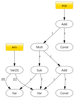
(a) A Concrete Heap.

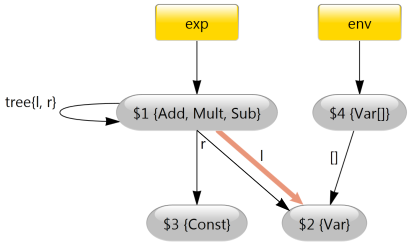
(b) Corresponding Abstract Heap.

Figure 1: Concrete and Abstract Heap

Figure 1(b) shows the corresponding normal form (see section 3) abstract heap for this concrete heap. To ease discussion we label each node in a graph with a unique node id ($id). The abstraction summarizes the concrete objects into three regions. The regions are represented by the nodes in the abstract heap graph: (1) a node representing all interior recursive objects in the expression tree (Add, Mult, Sub), (2) a node representing the two Var objects, and (3) a node representing the two Const objects. The edges represent possible sets of non-null cross region pointers associated with the given abstract labels. Details about the order and branching structure of expression nodes are absent but other more general properties are still present. For example, the fact that there is no sharing or cycles among the interior expression nodes is apparent in the abstract graph by looking at the self-edge representing the pointers between objects in the interior of the expression tree. The label tree{l,r} on the self-edge expresses that pointers stored in the l and r fields of the objects represented by node $1$ form a tree structure.

The abstract graph maintains another useful property of the expression tree, namely that no Const object is referenced from multiple expression objects. On the other hand, several expression objects might point to the same Var object. The abstract graph shows this possible non-injectivity using wide orange colored edges (if color is available), whereas normal edges indicate injective pointers. Similarly the edge from node $4$ (the env array) to the set of Var objects represented by node $2$ is injective, not shaded and wide. This implies that there is no aliasing between the pointers stored in the array, i.e. every index in the array contains a pointer to a unique object. Additionally, the abstract heap, via a combination of reachability, shape, and sharing information, shows there is no aliasing on any distinct pair of paths starting from exp and ending with a dereference of the r field. This can be deduced from the fact that node 1 is a tree layout, so there is no aliasing internally on either the l or r fields, and that both outgoing edges r edges are injective (narrow and unshaded). Since we know all paths through the tree do not alias (lead to different objects) this implies the final dereferences of the r fields, which can only contain injective pointers to Const or Var objects, do not alias either.

3 Normal Form

Given the definitions for the abstract heap it is clear that the domain is infinite. This allows substantial flexibility when defining the transfer functions and more precise results when analyzing straight line blocks of code. However, it is problematic when defining the merge/equality operations and can result in the final analysis having an unacceptably large computational cost. To prevent this we define an efficiently computable normal form, $O((N+E)*\mathit{log}(N))$ where $N$ is the number of nodes in the abstract heap graph and $E$ is the number of edges. The normal form ensures that the set of normal form abstract heaps for any given program is finite and that the abstract heaps in this set can easily be merged and compared.

The normal form leverages the idea that locally (within a basic block or method call) invariants can be broken and subtle details are critical to program behavior but before/after these local components invariants should be restored. The basis for the normal form, and the selection of what are important properties to preserve, comes from studies of the runtime heap structures produced in object-oriented programs [31, 2]. Thus we know that, in general, these definitions are well suited to capturing the fundamental structural properties of the heap that are of interest while simplifying the structure of abstract heaps and discarding superfluous details.

Definition 1 (Normal Form)

We say that the abstract heap is in normal form iff:

1. All nodes are reachable from a variable or static field.

2. All recursive structures are summarized (Definition 2).

3. All equivalent successors are summarized (Definition 4).

4. All variable/global equivalent targets are summarized (Definition 5).

That is there are no unreachable nodes and structurally the abstract heap represents the congruence closure of the recursive structure, equivalent successor, and equivalent target relations.

While the normal form definition is fundamentally driven by heuristics derived from empirical studies of the heap structures in real programs (and thus one could imagine a number of variants) there are three key properties that it possesses: (1) the resulting abstract heap graph has a bounded depth, (2) each node has a bounded out degree, and (3) for each node the possible targets of the abstract addresses associated with it are unique wrt. the label and the types in the target nodes. The first two properties ensure that the number of abstract heaps in the normal form set are finite, while the third allows us to define efficient merge and compare operations (section 4).

3.1 Equivalence Partitions

As each of the properties (recursive structures, ambiguous successors, and ambiguous targets) are defined in terms of, congruence between abstract nodes the transformation of an abstract heap into the corresponding normal form is fundamentally the computation of a congruence closure over the nodes in the abstract heap followed by merging the resulting equivalence sets. Thus, we build a map from the abstract nodes to equivalence sets (partitions) using a Tarjan union-find structure. Formally $\Pi:\widehat{\mathsf{Ob}}\rightarrow\{\pi_{1},\ldots,\pi_{k}\}$ where $\pi_{i}\in 2^{\widehat{\mathsf{Ob}}}$ and $\{\pi_{1},\ldots,\pi_{k}\}$ are a partition of $\widehat{\mathsf{Ob}}$. The union-find structure can also be used to maintain the set of all the types associated with the nodes in a partition ($\bigcup_{n\in\pi}\widehat{\mathsf{Ty}}(n)$). Initially the partition is set as a singleton (i.e., $\forall n\in\widehat{\mathsf{Ob}}\,.\,\Pi(n)=\{n\}$).

The first step in computing the normal form is to identify any nodes that may be parts of unbounded depth structures. This is accomplished by examining the type system for the program that is under analysis and identifying all the types that are part of the same recursive type definitions. This is a commonly used technique [4, 28, 9] and ensures that any heap graph produced has a finite depth. We say types $\tau_{1}$ and $\tau_{2}$ are recursive ($\tau_{1}\sim\tau_{2}$) if they are part of the same recursive type definition.

Definition 2 (Recursive Structure)

Given two partitions $\pi_{1}$ and $\pi_{2}$ we define the recursive structure congruence relation as:

$$\pi_{1} \equiv_{r}^{\Pi}\pi_{2}\Leftrightarrow\exists\tau_{1}\in\textstyle{\bigcup_{n_{1}\in\pi_{1}}}\widehat{\mathsf{Ty}}(n_{1}),\tau_{2}\in\textstyle{\bigcup_{n_{2}\in\pi_{2}}}\widehat{\mathsf{Ty}}(n_{2})\,.\,\tau_{1}\sim\tau_{2}$$

$$\land\exists n\in\pi_{1},\widehat{l}\in\widehat{\mathsf{Fld}}(\widehat{\mathsf{Ty}}(n))\,.\,\widehat{\mathsf{Trgts}}(\widehat{\sigma}(n.\widehat{l}))\cap\pi_{2}\neq\emptyset$$

The other part of the normal form computation is to identify any partitions that have equivalent successors and variables that have equivalent targets. Both of these operations depend on the notion of a successor partition which is based on the underlying structure of the abstract heap graph: $\pi_{1}\text{ a successor of }\pi_{2}\text{ and }\widehat{l}\Leftrightarrow\exists n_{2}\in\pi_{2}\,.\,\widehat{\mathsf{Trgts}}(\widehat{\sigma}(n_{2}.\widehat{l}))\cap\pi_{1}\neq\emptyset$.

Definition 3 (Partition Compatibility)

We define the relation Compatible($\pi_{1}$, $\pi_{2}$) as: $\emph{Compatible}(\pi_{1},\pi_{2})\Leftrightarrow\bigcup_{n^{\prime}\in\pi_{1}}\widehat{\mathsf{Ty}}(n^{\prime})\cap\bigcup_{n^{\prime}\in\pi_{2}}\widehat{\mathsf{Ty}}(n^{\prime})\neq\emptyset$.

Definition 4 (Equivalent Successors)

Given $\pi_{1}$, $\pi_{2}$ which are successors of $\pi$ on labels $\widehat{l}_{1}$, $\widehat{l}_{2}$ we define the relation equivalent successors on them as: $\pi_{1}\equiv_{s}^{\Pi}\pi_{2}\Leftrightarrow\widehat{l}_{1}=\widehat{l}_{2}\land\emph{Compatible}(\pi_{1},\pi_{2})$.

Definition 5 (Equivalent on Targets)

Given a root $r$ (a variable or a static field) and two partitions $\pi_{1}$, $\pi_{2}$ where $r$ refers to a node in $\pi_{1}$ and a node in $\pi_{2}$ we define the equivalent targets relation as: $\pi_{1}\equiv_{t}^{\Pi}\pi_{2}\Leftrightarrow\emph{Compatible}(\pi_{1},\pi_{2})\land(\text{r is a static field}\lor\pi_{1},\pi_{2}\text{ only have local var predecessors})$.

Using the recursive structure relation and the equivalent successor (target) relations we can efficiently compute the congruence closure over an abstract heap producing the corresponding normal form abstract heap (Definition 2). This computation can be done via a standard worklist algorithm that merges partitions that contain equivalent nodes and can be done in $O((N+E)*\mathit{log}(N))$ time where $N$ is the number of abstract nodes in the initial abstract heap, and $E$ is the number of abstract addresses in the heap.

3.2 Computing Summary Nodes

After partitioning the nodes in the graph with the congruence closure computation we need to merge all the nodes in each partition into a summary node. The resulting summary node should safely summarize the properties of the all the nodes in the partition. Similarly, we may need to update target and injectivity information for the summary nodes in the abstract store. Given a node partition ($\pi$) that we want to replace with a new summary node ($n_{s}$) we use the following to compute the abstract properties for the summary node and new abstract store $\widehat{\sigma}_{s}$:

$$n_{s}=(\widehat{\iota}_{\emph{frsh}},\sqcup_{\emph{type}}(\pi),\sqcup_{\emph{shape}}(\pi),\{[\widehat{l}\mapsto\widehat{a_{\widehat{l}}}]\;|\;\widehat{l}\in\widehat{\mathsf{Fld}}(\sqcup_{\emph{type}}(\pi)),\widehat{a_{\widehat{l}}}\text{ a fresh address}\})$$

$$\quad\text{where }\widehat{\iota}_{\emph{frsh}}\text{ is a fresh node identifier in }\mathsf{NID}$$

$$\widehat{\sigma}_{s}=\emph{MergeStore}(\widehat{\sigma}_{s},\widehat{l},\pi)\text{ for each }\widehat{l}\in\widehat{\mathsf{Fld}}(\sqcup_{\emph{type}}(\pi))$$

$$\sqcup_{\emph{type}}(\pi)=\bigcup_{n\in\pi}\widehat{\mathsf{Ty}}(n)$$

Once this merge is complete we can update the information on the abstract addresses associated with each variable in $\widehat{\mathsf{Env}}$ by replacing any nodes in the target sets with the appropriate newly created summary nodes.

Shape.

The Shape information is non-trivial to merge as it depends both on the shapes of the individual nodes that are being grouped and also on the connectivity properties between them. We first perform a traversal of the subgraph of the partition and the (non-self) abstract targets between them. Then based on the discovery of back, cross, or tree references (in a graph theoretic sense) and if any of these abstract storage location are not injective we compute the shape as $\sqcup_{\emph{shape}}(\pi)$ $=$ $\emph{struct}(\pi)\sqcup\bigsqcup_{n\in\pi}\widehat{\mathsf{Sh}}(n)$ where :

$$\emph{struct}(\pi)=\left\{\begin{array}[]{cl}\mathsf{none}&\text{ if }\emph{No Internal Edges Exist}\\ \mathsf{tree}&\text{ if }\forall n\in\pi,\widehat{l}\in\widehat{\mathsf{Fld}}(\widehat{\mathsf{Ty}}(n))\,.\,\lnot\widehat{\mathsf{Inj}}(\widehat{\sigma}(n.\widehat{l}))\land n.\widehat{l}\emph{ a Tree Edge in }\pi\\ &\quad\land(\widehat{\mathsf{Sh}}(n)=\mathsf{none}\lor\forall n^{\prime}\in\widehat{\mathsf{Trgts}}(\widehat{\sigma}(n.\widehat{l}))\cap\pi\,.\,\widehat{\mathsf{Sh}}(n^{\prime})=\mathsf{none})\\ \mathsf{any}&\text{ otherwise }\\ \end{array}\right.$$

Injectivity and Abstract Targets.

Given a mapping from the partitions to the new summary nodes, $\Phi:\emph{Img}(\Pi)\rightarrow\{n_{s_{1}},\ldots,n_{s_{k}}\}$, then for each label, $\widehat{l}$, and abstract address, $\widehat{a_{\widehat{l}}}$, that may appear in a summary node, $n_{s}$, we set the values in the abstract store as:

$$\emph{MergeStore}(\widehat{\sigma}_{s},\widehat{l},\pi)=\widehat{\sigma}_{s}+[\widehat{a_{\widehat{l}}}\mapsto(\emph{inj},\emph{trgts})]\text{ where}$$

$$\quad\emph{trgts}=\{\Phi(\Pi(n^{\prime}))\;|\;n^{\prime}\in\textstyle{\bigcup_{n\in\pi}}\widehat{\mathsf{Trgts}}(\widehat{\sigma}(n.\widehat{l}))\}$$

$$\quad\emph{inj}=\forall n\in\pi\,.\,\widehat{\mathsf{Inj}}(\widehat{\sigma}(n.\widehat{l}))\land\forall n^{\prime}\in\pi\setminus\{n\}\,.\,\widehat{\mathsf{Trgts}}(\widehat{\sigma}(n_{1}.\widehat{l}))\cap\widehat{\mathsf{Trgts}}(\widehat{\sigma}(n_{2}.\widehat{l}))=\emptyset$$

Injectivity is the logical conjunction of the injectivity of all the source label locations, and that the respective targets sets of the nodes that are merged do not overlap. In the case where the target sets do overlap, i.e., two distinct nodes have abstract labels/addresses that contain the same node, the resulting address may not only be associated with injective pointers. Thus, the injectivity value is conservatively set to false (i.e., not injective). The target set is simply the remapping of the old nodes in the target sets to the appropriate newly created summary nodes.

From the definitions of the summary node computations and the update of the abstract store locations the preservation of the safety of the abstraction is straight forward to check via case enumeration. It is also clear that each partition is processed once in the normal form computation (and similarly the addresses in the abstract store are each only visited a constant number of times). Thus, the cost of computing the summaries can be done in linear time. Finally, as the congruence closure over given a graph is unique the resulting normal form graph, as defined here, is also unique.

3.3 Normal Form on Example Heap

We can see how this normal form works by using it to transform the concrete heap in Figure 1(a) into its normal form abstract representation. This can be done by first creating an abstract heap graph that is isomorphic to the concrete heap (i.e., create a node for each concrete object and set the appropriate targets in the abstract store for each concrete pointer). The resulting isomorphic abstract heap is shown in Figure 2.

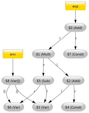
Figure 2: Isomorphic Abstract Heap.

The normal form partition for the abstract heap in Figure 2 identifies the nodes with the Add, Sub, and Mult types as being in the same partition (they are part of the same recursive structure). The presence of this partition will then cause all of the nodes with Const type (nodes $4$, $7$) to be identified as equivalent successors of the tree partition. Finally, either due to the tree partition or the fact that all the nodes with Var type (nodes $3$, $6$) have references to them from node $8$ (the Var[]) will cause all the partitions associated with Var types being identified as equivalent successors. Thus the final partitioning after the congruence closure is:

$$\mu^{-1}\left\{\begin{array}[]{lr}\pi_{1}:\{n_{0},n_{1},n_{2},n_{5}\}\\ \pi_{2}:\{n_{3},n_{6}\}\\ \pi_{3}:\{n_{4},n_{7}\}\\ \pi_{4}:\{n_{8}\}\\ \end{array}\right.$$

Given this set of partitions the computation of the various properties is straight forward. The Shape for the partitions containing the Var, Const and Var[] nodes is trivial to compute as there are no internal references between the nodes in these partitions. The shape computation for the partition ($\pi_{1}$) containing the nodes in the expression structure requires a traversal of the four nodes, and as there are no internal cross or back edges the layout for this is $\mathsf{tree}$.

In computing the new summary abstract store properties for the abstract address associated with the expression tree partition ($\pi_{1}$) and the label l there are two nodes ($n_{2}$ and $n_{5}$) that refer to the same node ($n_{3}$) in partition $\pi_{2}$. Thus this abstract storage location is set to not injective (false). However, for the label r from partition $\pi_{1}$ the target sets are disjoint and thus the injectivity in the abstract store is set to true (injective). Similarly, the store location for the label [] out of the partition $\pi_{4}$ representing the targets of the pointers stored in the env array is set as injective. This results in the normal form abstract heap shown in Figure 1(b).

4 Domain Operations

Given the normal form in section 3 we can define an efficiently computable abstract equality operation ($\widehat{=}$) and upper approximation ($\widetilde{\sqcup}$) operator on the normal form abstract heaps. Since the set of normal form abstract heaps is finite (for a given program) we do not need a widening operator. Both operations can be performed efficiently, $O(N+E)$ for equality and $O((N+E)*\mathit{log}(N))$ for the upper approximation.

Abstract Equality.

To enable efficient comparison we only define abstract equality on the normal forms of the abstract heap states and we ensure it satisfies the property:

$$(\widehat{\mathsf{Env}}_{1},\widehat{\sigma}_{1},\widehat{\mathsf{Ob}}_{1})\widehat{=}(\widehat{\mathsf{Env}}_{2},\widehat{\sigma}_{2},\widehat{\mathsf{Ob}}_{2})\Rightarrow\gamma((\widehat{\mathsf{Env}}_{1},\widehat{\sigma}_{1},\widehat{\mathsf{Ob}}_{1}))=\gamma((\widehat{\mathsf{Env}}_{2},\widehat{\sigma}_{2},\widehat{\mathsf{Ob}}_{2}))$$

Since the set of normal form abstract graphs we use in the fixpoint computation is finite this is sufficient to guarantee termination and safety of the analysis.

Given two abstract heaps $(\widehat{\mathsf{Env}}_{1},\widehat{\sigma}_{1},\widehat{\mathsf{Ob}}_{1})$ and $(\widehat{\mathsf{Env}}_{2},\widehat{\sigma}_{2},\widehat{\mathsf{Ob}}_{2})$ we first determine if they are structurally isomorphic (i.e., is there an isomorphism that respects variable and field labels), then we check that all abstract node and store properties in $(\widehat{\mathsf{Env}}_{2},\widehat{\sigma}_{2},\widehat{\mathsf{Ob}}_{2})$ have the same values in $(\widehat{\mathsf{Env}}_{1},\widehat{\sigma}_{1},\widehat{\mathsf{Ob}}_{1})$ under the isomorphism.

To efficiently compute the needed isomorphism we use a property of the abstract graphs established by the normal form definition (Definition 1). By this definition we know that each node is reachable from a root location (a local variable or a static field), thus if an isomorphism exists it can be found by matching from the roots. Further, we know that for each abstract address in the store if there is more than one element in the target set then each of these targets must have non-overlapping sets of types (from the definition of Compatible, Definition 3). Thus, to compute an isomorphism between two graphs we can simply start pairing the local and static roots and then process the abstract structure in a breadth first manner, pairing up nodes based on abstract labels and type sets of the targets, leading to new pairings. This either results in an isomorphism between the two structures, $\phi$, or it reaches a point where no match is possible and fails without backtracking. If we find an isomorphism $\phi$ then we check the equivalence of the abstract nodes and store as follows:

$$(\widehat{\mathsf{Env}}_{1} ,\widehat{\sigma}_{1},\widehat{\mathsf{Ob}}_{1})=_{\phi}(\widehat{\mathsf{Env}}_{2},\widehat{\sigma}_{2},\widehat{\mathsf{Ob}}_{2})\Leftrightarrow$$

$$\forall n\in\widehat{\mathsf{Ob}}_{1}\,.\,\widehat{\mathsf{Ty}}(n)=\widehat{\mathsf{Ty}}(\phi(n))\land\widehat{\mathsf{Sh}}(n)=\widehat{\mathsf{Sh}}(\phi(n))$$

$$\quad\land\forall\widehat{l}\in\widehat{\mathsf{Fld}}(\widehat{\mathsf{Ty}}(n))\,.\,\widehat{\mathsf{Inj}}(\widehat{\sigma}_{1}(n))=\widehat{\mathsf{Inj}}(\widehat{\sigma}_{2}(\phi(n)))$$

Upper Approximation.

The upper approximation operation takes two abstract heaps and produces a new abstract heap that is an over approximation of all the concrete heap states that are represented by the two input abstract heaps. In the standard abstract interpretation formulation this is typically the least element that is also an over approximation. However, to simplify the computation we do not enforce this property (formally we define an upper approximation instead of a join). Our approach is to leverage the existing definitions from the normal form computation in the following steps.

Given two abstract heaps, $(\widehat{\mathsf{Env}}_{1},\widehat{\sigma}_{1},\widehat{\mathsf{Ob}}_{1})$ and $(\widehat{\mathsf{Env}}_{2},\widehat{\sigma}_{2},\widehat{\mathsf{Ob}}_{2})$ we can define the their merge by taking the union of the abstract node sets and the abstract stores in the usual way and then from this union we can compute the corresponding normal form as described in section 3.

$$(\widehat{\mathsf{Env}}_{1} ,\widehat{\sigma}_{1},\widehat{\mathsf{Ob}}_{1})\widehat{\sqcup}(\widehat{\mathsf{Env}}_{2},\widehat{\sigma}_{2},\widehat{\mathsf{Ob}}_{2})=\emph{Normalize}(\widehat{\mathsf{Env}}_{m},\widehat{\sigma}_{m},\widehat{\mathsf{Ob}}_{1}\uplus\widehat{\mathsf{Ob}}_{2})\text{ where}$$

$$\widehat{\mathsf{Env}}_{m}=\{[v\mapsto\widehat{a_{v}}]\;|\;v\in\emph{Dom}(\widehat{\mathsf{Env}}_{1}\cup\widehat{\mathsf{Env}}_{2}),\widehat{a_{v}}\text{ a fresh address}\}$$

$$\widehat{\sigma}_{m}=\widehat{\sigma}_{1}\uplus\widehat{\sigma}_{2}\uplus\{[\widehat{a_{v}}\mapsto(\emph{true},\emph{trgts}_{v})]\;|\;[v\mapsto\widehat{a_{v}}]\in\widehat{\mathsf{Env}}_{m}\}$$

$$\quad\emph{trgts}_{v}=\widehat{\mathsf{Trgts}}(\widehat{\sigma}_{1}(\widehat{\mathsf{Env}}_{1}(v)))\cup\widehat{\mathsf{Trgts}}(\widehat{\sigma}_{2}(\widehat{\mathsf{Env}}_{2}(v)))$$

5 Abstract Transfer Functions

Given the expressive Shape Analysis Style domain defined in subsection 2.2 the next step is to define a set of transfer functions that simulate the effects of various program statements on the abstract heaps. Our goal is to construct these definitions in a Points-To Analysis Style, using weak updates and simple set operations while still precisely modeling the effects of each statement on the heap state. In order to focus on the fundamental aspects of the analysis we present the results on a simple object-oriented language with the standard set of allocation, load, and store operations. However, in practice the approach can be extended in a natural way to handle a much richer language. Our implementation for .Net bytecode (section 6) handles features such as struct types, references to the stack, pointers to the interior of objects, and function pointers.

Table 1 shows the transition semantics for the statements that are the most interesting from the standpoint of memory analysis (see the companion paper [29] for a full description of how the interprocedural analysis is performed). In order to focus on the central ideas we ignore issues with null-pointer dereferences, array out-of-bounds errors, etc. In most cases the abstract transfer functions are the natural translations of the concrete semantic operations, and are very similar to the set of transfer functions seen in a standard points-to analysis [33, 38, 42]. However, there are a number of important differences from a standard formulation of points-to analysis transfer functions, of particular interest are the allocation, load, and store operations.

$\displaystyle v=\texttt{alloc type: }(\widehat{\mathsf{Env}},\widehat{\sigma},\widehat{\mathsf{Ob}})\leadsto(\widehat{\mathsf{Env}},\widehat{\sigma}^{\prime},\widehat{\mathsf{Ob}}^{\prime})\text{ where}$ $\displaystyle\quad n=(\widehat{\iota}_{\emph{frsh}},\texttt{type},\mathsf{none},\{\widehat{l}\rightarrow\widehat{a_{\widehat{l}}}\;|\;\widehat{l}\in\widehat{\mathsf{Fld}}(\{\texttt{type}\}),\widehat{a_{\widehat{l}}}\text{ fresh address}\})$ $\displaystyle\quad\quad\text{where }\widehat{\iota}_{\emph{frsh}}\text{ is a fresh node identifier from }\mathsf{NID}$ $\displaystyle\quad\widehat{\sigma}^{\prime}=\widehat{\sigma}+[\widehat{\mathsf{Env}}(v)\mapsto(\emph{true},\{n\})]+\{[n.\widehat{l}\mapsto(\emph{true},\emptyset)]\;|\;\widehat{l}\in\widehat{\mathsf{Fld}}(\{\texttt{type}\})\}$ $\displaystyle\quad\widehat{\mathsf{Ob}}^{\prime}=\widehat{\mathsf{Ob}}\uplus\{n\}$ $\displaystyle v=v^{\prime}.\widehat{l}\texttt{: }(\widehat{\mathsf{Env}},\widehat{\sigma},\widehat{\mathsf{Ob}})\leadsto(\widehat{\mathsf{Env}},\widehat{\sigma}^{\prime},\widehat{\mathsf{Ob}})\text{ where}$ $\displaystyle\quad v^{\prime}_{\emph{trgts}}=\widehat{\mathsf{Trgts}}(\widehat{\sigma}(\widehat{\mathsf{Env}}(v^{\prime})))$ $\displaystyle\quad\widehat{\sigma}^{\prime}=\widehat{\sigma}+[\widehat{\mathsf{Env}}(v)\mapsto(\emph{true},\bigcup_{n\in v^{\prime}_{\emph{trgts}}}\widehat{\mathsf{Trgts}}(\widehat{\sigma}(n.\widehat{l})))]$ $\displaystyle v.\widehat{l}=v^{\prime}\texttt{: }(\widehat{\mathsf{Env}},\widehat{\sigma},\widehat{\mathsf{Ob}})\leadsto(\widehat{\mathsf{Env}},\widehat{\sigma}^{\prime},\widehat{\mathsf{Ob}})\text{ where}$ $\displaystyle\quad v_{\emph{trgts}}=\widehat{\mathsf{Trgts}}(\widehat{\sigma}(\widehat{\mathsf{Env}}(v)))$ $\displaystyle\quad v^{\prime}_{\emph{trgts}}=\widehat{\mathsf{Trgts}}(\widehat{\sigma}(\widehat{\mathsf{Env}}(v^{\prime})))$ $\displaystyle\quad\forall n\in v_{\emph{trgts}}\,.\,\text{if }n\in v^{\prime}_{\emph{trgts}}\text{ then }\widehat{\mathsf{Sh}}(n)\leftarrow\mathsf{any}$ $\displaystyle\quad\quad\widehat{\sigma}^{\prime}=\widehat{\sigma}+[n.\widehat{l}\mapsto(\emph{inj},\widehat{\mathsf{Trgts}}(\widehat{\sigma}(n.\widehat{l}))\cup v^{\prime}_{\emph{trgts}})]$ $\displaystyle\quad\quad\text{where }\emph{inj}=\widehat{\mathsf{Inj}}(\widehat{\sigma}(n.\widehat{l}))\land\widehat{\mathsf{Trgts}}(\widehat{\sigma}(n.\widehat{l}))\cap v^{\prime}_{\emph{trgts}}=\emptyset$

Table 1: Abstract Semantics

Allocate.

The definition of the allocation operation plays a key role in the functioning of the analysis. As opposed to the usual points-to definition which will reuse nodes in the abstract heap based on some context token, ranging from simple allocation type or line number through sophisticated object-sensitive constructions, our definition of the allocation operation always creates a fresh node. In this sense the definition closely resembles the constructions used in shape style analyses.

The creation of a fresh node for each visit to an allocation site is critical to allowing the analysis to later model stores into/of this object and the impact on injectivity and shape. Any finite naming scheme creates situations where there will be spurious reuse of a node, which will cause the loss of injectivity and/or shape information (e.g., in the store operation or the normal form summary computation). Of course the creation of a new node at each visit to an allocation site creates a potential problem with the termination of the analysis as the abstract heap state may grow without bound. However, by applying the normal form operation from section 3 at each control flow join point and at each call site we can be sure of the termination of the analysis as the set of graphs that are in normal form is finite.

Load.

The load operation is a simple translation of the concrete semantics where the target set that is stored into the variable is the union of the target sets of the appropriate fields and objects. However, as a variable location always contains a single pointer we can strongly update the target set and set the associated injective value to true.

Store.

The store operation plays a central role in the analysis as it is where special care needs to be taken to update the injectivity and shape information. It first gathers all the possible objects that may be stored into ($v_{\emph{trgts}}$) and all the possible objects that it may be storing references to ($v^{\prime}_{\emph{trgts}}$). In the update step we compute new values for the possible shape, the new target node set, and the new injectivity value. The shape information is handled by checking if the node we are storing into is in the set of possible targets. If it is then we may be modifying the shape of the data structure represented by the node we are updating. It is possible to perform additional checks to be more precise in updating the shape information but we simply set the shape to the top value ($\mathsf{any}$) in the case that a self store occurs. If there is no self store then the shape is unchanged.

The update to the abstract store involves taking the union of the old target set and the new target set (weakly updating the target set) and computing a new injectivity value. There are two cases we need to check to determine the new injectivity value. The first is if the old injectivity value was false, in which case we leave it as false. The second is if the new target set and the old target set overlap, in which case we cannot guarantee that the address is only associated with injective pointers. Again in this case we conservatively set the result as not injective. If neither of these cases occur then we mark the abstract address as containing injective pointers (i.e., the injective value is true).

6 Implementation and Evaluation

To facilitate comparisons with other work we have primarily selected benchmarks that are direct C# ports of commonly used Java benchmarks including programs from Jolden [21], the db and raytracer programs from SPEC JVM98 [39], and the luindex and lusearch programs from the DaCapo suite [21]. Additionally we have analyzed the heap abstraction code, runabs, from [31]. In practice we translate the .Net assemblies to a simplified IR (intermediate representation) which allows us remove most .Net specific idioms from the core analysis and simplifies later analysis steps. Our test machine is an Intel i7 class processor at $2.66$ GHz with $2$ GB of RAM available. We use the standard $32$ bit .Net JIT and runtime framework provided by Windows $7$. The domain, operations, and data flow analysis algorithms are all implemented in C# and are publicly available.

Client Applications
The analysis in this paper tracks general classes of properties that have shown, in past work, to be both relevant and useful in a wide range of client applications [12, 30, 14, 15, 24, 16, 27]. However, we have performed additional small scale implementations and case studies with the analysis results to ensure that the particulars of the domain defined in this paper are useful for these types of optimization and program understanding applications. These case studies include:

• The introduction of thread-level parallelization, as in [30], to obtain a $3\times$ speedup for bh on our quad-core machine.

• Data structure reorganization to improve memory usage and automated leak detection, as in [31], to obtain over a $25$% reduction in live memory in raytrace.

• The computation of ownership information for object fields, as in [27], identifying ownership properties for $22$% of the fields and unique memory reference properties for $47$% of the fields in lusearch.

However, we want to examine the quantitative precision of the analysis in a way that is free from biases introduced by the selection of a particular client application. Thus, we examine the precision of the static analysis relative to the abstract heaps derived from concrete executions of the program. This notion of precision is a more general measurement of the possible imprecision due to the use of weak-updates and simple points-to style transfer functions than the use of a specific client application (which may hide precision losses that happen not to matter for the particular client).

Quantitative Precision
We define precision relative to a hypothetical perfect analysis which uses the same abstract domain from section 2 but that is able to perfectly predict the effects of every program operation. Since we cannot actually build such an analysis we approximate it by collecting and abstracting the results of concrete executions. By definition this collection of results from the concrete execution is an under approximation of the universal information we want to compute, and in the limit of execution of all possible inputs is identical. Formally, given a method and a set of concrete heaps $\{h_{1},\ldots,h_{k}\}$ and a set of abstract heaps $\{\widehat{h}_{1},\ldots,\widehat{h}_{j}\}$ we can compute differences between $\bigsqcup_{h\in\{h_{1},\ldots,h_{k}\}}\alpha(h)$ and $\bigsqcup\{\widehat{h}_{1},\ldots,\widehat{h}_{j}\}$. This gives an unbiased measure of how close our results are to the optimal solution, wrt. the abstract domain we are working with in a way that is independent of peculiarities of a client application or other analysis technique.

One possible concern with this approach is that the base abstract domain may be very coarse, i.e., $\bigsqcup_{h\in\{h_{1},\ldots,h_{k}\}}\alpha(h)$ is always $\top$ or another very imprecise value. To account for this we report the average percentage of properties (shape and injectivity) that the runtime result marks as precise ($\mathsf{none}$ or $\mathsf{tree}$ and injective) in the models (the Runtime Precise Rate group in Table 2). This table shows that in practice the domain achieves a very high rate of precise identification of shape values, on average over $90$% or more of nodes are precisely identified (the Shape column), and a similarly high rate of precise injectivity values, on average nearly $90$% of the edges are identified as being injective (the Injectivity column). For reference the example abstract heap, Figure 1(b), would have a $100$% precise shape rate and a $75$% precise injectivity rate. Thus, we can see that in general the base domain is exceptionally effective in representing the heap properties we are interested and is an effective baseline for comparison against.

	Static Match Rate			Runtime Precise Rate
Benchmark	Region	Shape	Injectivity	Shape	Injectivity
power	100%	100%	100%	100%	100%
bh	100%	90%	87%	100%	100%
db	100%	100%	81%	100%	100%
raytracer	80%	85%	83%	89%	98%
luindex	95%	95%	82%	100%	91%
lusearch	93%	90%	84%	96%	89%
runabs	97%	98%	87%	94%	90%

Table 2: Static Match is percentage of each property correctly predicted by the static analysis when compared to perfect analysis. Runtime Precise is the percentage of properties that the perfect analysis captures precisely.

Table 2 shows the results of comparing the results from our perfect analysis with the results from the static analysis analysis described in this paper. In this table we report the percentage of properties in the static analysis results that are the same as reported by the runtime analysis for regions, shapes, and injectivity values. The region percentage (the Region column) is number of nodes that can be exactly matched between the statically computed and runtime result structure. Using this matching we then compute the percentage of the shape and injectivity properties that are precisely identified by the static analysis (the Shape and Injectivity columns). Overall the results show that the analysis is able to extract a large percentage of the properties that can be expressed via the selected abstract domain (in general with a rate of $80$% to $90$%). Thus, in general the use of weak-updates and points-to style transfer functions result in only small losses in precision when analyzing the behavior of the program and the effects of various operations on the state of the heap.

Analysis Performance
We next examine the cost of running the analysis in this paper in conjunction with the interprocedural analysis described in the companion paper [29]. For each benchmark we list the number of bytecode instructions, the number of classes, and the number of methods that each program contains after being translated into the internal IR. These numbers exclude much of the code that would normally be part of the runtime system libraries. This is due to the fact that during the translation from .Net bytecode to the internal IR code which is never referenced is excluded. Additionally for the builtin types/methods that are used the implementations are often replaced by simplified versions or specialized domain operations.

Benchmark Statistics				Analysis Cost
Name	Insts	Classes	Methods	Time	Mem
power	3,298	43	320	0.09s	11MB
bh	3,723	45	351	0.42s	14MB
db	2,873	42	315	0.21s	12MB
raytracer	9,808	65	476	6.72s	32MB
luindex	26,852	246	1747	12.1s	53MB
lusearch	33,632	272	1919	64.3s	130MB
runabs	27,875	253	1894	10.4s	60MB

Table 3: Benchmark statistics and aggregate performance of the analysis.

The last two columns of Table 3 show the aggregate performance of the analysis on the benchmark set. The timing measurements exclude the time required to startup and read/transform the source program into the internal IR. These performance results show that the analysis described in this work is quite efficient and capable of analyzing complex programs. In the case of luindex (a fairly direct translation of the Java version from the DaCapo suite) the analysis requires only $12$ seconds while recently reported results on context-sensitive points to analyses [38] reports analysis times ranging between $67$ and $179$ seconds depending on the amount and type of object-sensitivity used (and $37$ seconds with an insensitive analysis). But more importantly, as memory use frequently is a major scalability wall, are the low memory requirements. Despite performing the equivalent of full call graph cloning for large parts of the analysis and being partially context sensitive on the remainder, the analysis presented in this paper uses less than 130 MB of memory when analyzing any of the benchmarks.

7 Related Work

From the viewpoint of the analysis in this paper work on points-to analysis can be seen as falling into two categories, flow-insensitive, and flow-sensitive. Flow-insensitive analyses fundamentally prioritize speed and scalability over precision and thus are much faster but produce much less sophisticated information [40, 18]. In particular these approaches can now scale to millions of lines of code with analysis times on the order of a few seconds or less [18]. The second class of points-to style analyses are more precise, tracking information in a flow-sensitive manner [26, 19] and often employing techniques to track information in a way that is sensitive to different call sites, either via a context-sensitive or object-sensitive approach [38, 33, 22]. While these analyses are more precise than flow insensitive points-to analyses they do not express general shape or sharing properties. However, due to the way that context is tracked they can produce more precise points-to information in some cases than the analysis in this paper and it is an open question if object sensitive techniques can be used to improve on the results in this paper. Somewhat surprisingly these context (or object) sensitive analyses can be slower (and use more memory) than the analysis in this paper.

Work on memory analysis by Latter et. al. [23, 25] is based on a modular approach which first builds local shape graphs for each method via a local flow-insensitive points to analysis, and then merges (and clones as needed) these local graphs via a context-sensitive interprocedural analysis to produce the final result. Due to the modular and flow insensitive nature of the analysis it is very efficient, capable of analyzing large C++ programs in seconds. The use of a flow-insensitive and a local points-to analysis limits the range of properties that can be extracted and the precision of the analysis. However, as the focus of this work was scalability (instead of expressivity) it provides an interesting contrast in design decisions to the hybrid analysis proposed in this paper. Similarly the work in [17, 11] mixes shape and points-to analysis by first partitioning the heap into regions via a flow-insensitive points-to analysis followed by performing shape analysis based on these partitions. The work of Ghiya and Hendren [12] uses points-to and basic reachability predicates to compute shape information and in Section 4.3 notes the challenges of using weak updates when analyzing shape properties. The results in this paper show that the problems described in [12] are not, in practice, fundamental impediments to computing precise shape and sharing information in modern object-oriented programs.

There is an extensive body of work on shape analysis [7, 37, 13, 43, 32, 14, 11, 35, 20], and while the work in presented in this paper eschews the use of materialization and case splitting in the abstract transfer functions, it borrows heavily from existing work in the design of the abstract domain and in the selection of properties it encodes. In particular the domain in this paper is based on the basic storage shape graph construction [7], which is then augmented with additional information on data structure shape [12] and sharing information (injectivity) [32]. However, as opposed to using a partitioning scheme based on type or allocation site as done in [7] (or in most work on points-to analysis) the approach in this paper always creates a fresh node in the graph during the allocation operation. This node is then grouped into other data structures as needed using a normal form operation based on connectivity and a set of equivalence relations on the properties of the nodes [43, 28]. The simplicity of the transfer functions in this work, as opposed to the more sophisticated shape analysis transfer functions, results in a much faster and more scalable analysis at the cost of a small amount of precision.

We note that existing shape style approaches do not currently scale to programs of this size/complexity. While [6, 11] have shown promise in scaling to large programs the techniques in [6] do not allow generalized sharing in the heap structures while the techniques in [11] do not handle programs that contain recursive data structures. Further, the programs that these approaches have been demonstrated on contain relatively shallow and small data structures and the code does not heavily employ recursion or dynamic dispatch. In contrast the approach in this paper does not place any constraints on the programs under analysis and the benchmarks in this evaluation contain a range of large and complex data structures that are connected in a variety of ways. The benchmark programs used in this paper also extensively employ dynamic dispatch and contain non-trivial recursive traversals of heap structures.

8 Conclusion

This paper introduced Structural Analysis, a novel memory analysis technique based on the combination of a shape analysis style abstract heap model, a normal form driven by empirical studies of heap structures in real-world object-oriented programs, and a set of points-to analysis style transfer functions. The resulting hybrid memory analysis is able to precisely identify various structures in memory and to track sharing, shape, and reachability relations on them. We believe that the combined scalability and precision of the hybrid shape and points-to analysis structure presents both immediate benefits and unique opportunities for future research. The development of an expressive and scalable heap analysis is a valuable contribution wrt. the wide range of other research that depends on information about the program heap. However, we also believe further work in the area of hybrid analysis approaches, such as adding object-sensitivity or integrating aspects from SMT or separation logic based approaches, will be fruitful areas of investigation. As such we believe the analysis presented in this paper represents the introduction of a significant new class of heap analysis and represents an important advancement in the state of the art in precise and scalable heap analysis techniques.

References

- [1] S. Albiz and P. Lam. Implementation and use of data structures in Java programs. http://patricklam.ca/dsfinder/, 2010.
- [2] E. Barr, C. Bird, and M. Marron. Collecting a Heap of Shapes. Technical Report MSR-TR-2011-135, Microsoft Research, Dec. 2011.
- [3] W. Benton and C. Fischer. Mostly-functional behavior in Java programs. In VMCAI, 2009.
- [4] J. Berdine, C. Calcagno, B. Cook, D. Distefano, P. O’Hearn, T. Wies, and H. Yang. Shape analysis for composite data structures. In CAV, 2007.
- [5] S. Blackburn, R. Garner, C. Hoffman, A. Khan, K. McKinley, R. Bentzur, A. Diwan, D. Feinberg, D. Frampton, S. Guyer, M. Hirzel, A. Hosking, M. Jump, H. Lee, J. Moss, A. Phansalkar, D. Stefanović, T. VanDrunen, D. von Dincklage, and B. Wiedermann. The DaCapo benchmarks: Java benchmarking development and analysis (2006-mr2). In OOPSLA, 2006.
- [6] C. Calcagno, D. Distefano, P. O’Hearn, and H. Yang. Compositional shape analysis by means of bi-abduction. In POPL, 2009.
- [7] D. Chase, M. Wegman, and K. Zadeck. Analysis of pointers and structures. In PLDI, 1990.
- [8] P. Cousot and R. Cousot. Systematic design of program analysis frameworks. In POPL, 1979.
- [9] A. Deutsch. Interprocedural may-alias analysis for pointers: Beyond k-limiting. In PLDI, 1994.
- [10] I. Dillig, T. Dillig, and A. Aiken. Precise reasoning for programs using containers. In POPL, 2011.
- [11] I. Dillig, T. Dillig, A. Aiken, and M. Sagiv. Precise and compact modular procedure summaries for heap manipulating programs. In PLDI, 2011.
- [12] R. Ghiya and L. Hendren. Is it a tree, a dag, or a cyclic graph? A shape analysis for heap-directed pointers in C. In POPL, 1996.
- [13] A. Gotsman, J. Berdine, and B. Cook. Interprocedural shape analysis with separated heap abstractions. In SAS, 2006.
- [14] S. Gulwani and A. Tiwari. An abstract domain for analyzing heap-manipulating low-level software. In CAV, 2007.
- [15] S. Guyer and K. McKinley. Finding your cronies: static analysis for dynamic object colocation. In OOPSLA, 2004.
- [16] S. Guyer, K. McKinley, and D. Frampton. Free-me: a static analysis for automatic individual object reclamation. In PLDI, 2006.
- [17] B. Hackett and R. Rugina. Region-based shape analysis with tracked locations. In POPL, 2005.
- [18] B. Hardekopf and C. Lin. The ant and the grasshopper: fast and accurate pointer analysis for millions of lines of code. In PLDI, 2007.
- [19] B. Hardekopf and C. Lin. Semi-sparse flow-sensitive pointer analysis. In POPL, 2009.
- [20] J. Jenista, Y. Eom, and B. Demsky. Using disjoint reachability for parallelization. In CC, 2011.
- [21] Jolden Suite. http://www-ali.cs.umass.edu/DaCapo/.
- [22] N. Jones and S. Muchnick. A flexible approach to interprocedural data flow analysis and programs with recursive data structures. In POPL, 1982.
- [23] C. Lattner and V. Adve. Data Structure Analysis: An Efficient Context-Sensitive Heap Analysis. Technical Report UIUCDCS-R-2003-2340, Computer Science Dept., Univ. of Illinois at Urbana-Champaign, Apr 2003.
- [24] C. Lattner and V. Adve. Automatic pool allocation: improving performance by controlling data structure layout in the heap. In PLDI, 2005.
- [25] C. Lattner, A. Lenharth, and V. Adve. Making context-sensitive points-to analysis with heap cloning practical for the real world. In PLDI, 2007.
- [26] O. Lhoták and K.-C. A. Chung. Points-to analysis with efficient strong updates. In POPL, 2011.
- [27] K.-K. Ma and J. Foster. Inferring aliasing and encapsulation properties for java. In OOPSLA, 2007.
- [28] R. Manevich, E. Yahav, G. Ramalingam, and M. Sagiv. Predicate abstraction and canonical abstraction for singly-linked lists. In VMCAI, 2005.
- [29] M. Marron, O. Lhoták, and A. Banerjee. Programming paradigm driven heap analysis. In CC, 2012.
- [30] M. Marron, M. Méndez-Lojo, M. Hermenegildo, D. Stefanovic, and D. Kapur. Sharing analysis of arrays, collections, and recursive structures. In PASTE, 2008.
- [31] M. Marron, C. Sanchez, Z. Su, and M. Fahndrich. Abstracting runtime heaps for program understanding. In Submission, 2011.
- [32] M. Marron, D. Stefanovic, M. Hermenegildo, and D. Kapur. Heap analysis in the presence of collection libraries. In PASTE, 2007.
- [33] A. Milanova, A. Rountev, and B. Ryder. Parameterized object sensitivity for points-to analysis for Java. ACM Trans. Softw. Eng. Methodol., 2005.
- [34] F. Nielson, H. Nielson, and C. Hankin. Principles of Program Analysis. Springer-Verlag New York, Inc., 1999.
- [35] X. Rival and B.-Y. E. Chang. Calling context abstraction with shapes. In POPL, 2011.
- [36] S. Sagiv, T. Reps, and R. Wilhelm. Solving shape-analysis problems in languages with destructive updating. In POPL, 1996.
- [37] S. Sagiv, T. Reps, and R. Wilhelm. Parametric shape analysis via 3-valued logic. In POPL, 1999.
- [38] Y. Smaragdakis, M. Bravenboer, and O. Lhoták. Pick your contexts well: understanding object-sensitivity. In POPL, 2011.
- [39] Standard Performance Evaluation Corporation. JVM98 Version 1.04, August 1998. http://www.spec.org/jvm98.
- [40] B. Steensgaard. Points-to analysis in almost linear time. In POPL, 1996.
- [41] C. Unkel and M. Lam. Automatic inference of stationary fields: a generalization of Java’s final fields. In POPL, 2008.
- [42] R. Wilson and M. Lam. Efficient context-sensitive pointer analysis for C programs. In PLDI, 1995.
- [43] H. Yang, O. Lee, J. Berdine, C. Calcagno, B. Cook, D. Distefano, and P. O’Hearn. Scalable shape analysis for systems code. In CAV, 2008.