Negative Quasi-Probability as a Resource for Quantum Computation

Abstract

A central problem in quantum information is to determine the minimal physical resources that are required for quantum computational speedup and, in particular, for fault-tolerant quantum computation. We establish a remarkable connection between the potential for quantum speed-up and the onset of negative values in a distinguished quasi-probability representation, a discrete analog of the Wigner function for quantum systems of odd dimension. This connection allows us to resolve an open question on the existence of bound states for magic-state distillation: we prove that there exist mixed states outside the convex hull of stabilizer states that cannot be distilled to non-stabilizer target states using stabilizer operations. We also provide an efficient simulation protocol for Clifford circuits that extends to a large class of mixed states, including bound universal states.

While it is widely believed that quantum computers can solve certain problems with exponentially fewer resources than their classical counterparts, the scope of the physical resources of the underlying quantum systems that enable universal quantum computation is not well understood. For example, for the standard circuit model of quantum computation, Vidal has shown that high-entanglement is necessary for an exponential speed-up Vidal (2003a); however, it is also known that access to high-entanglement is not sufficient Gottesman (1997). Moreover, in alternative models of quantum computation such as DQC1 Knill and Laflamme (1998), algorithms that may be performed on highly-mixed input states appear to be more powerful than classical computation even though there appears to be a negligible amount of entanglement in the underlying quantum system Datta et al. (2005). This suggests that large amounts of entanglement, purity or even coherence may not be necessary resources for quantum-computational speed-up. One of the central open problems of quantum information is to understand which sets of quantum resources are jointly necessary and sufficient to enable an exponential speed-up over classical computation. Any solution to this important problem may point to more practical experimental means of achieving the benefits of quantum computation.

The question of whether a restricted subset of quantum theory is still sufficient for a given task is meaningful when there is a specific context that divides the full set of possible quantum operations into two classes: the restricted subset of operations that are accessible or easy to implement and the remainder that are not. In such a context it is then natural to consider the difficult operations as resources and ask how much, if any, of these resources are required. For example, a common paradigm in quantum communication is that of two or more spatially separated parties for which local quantum operations and classical communication define a restricted set of operations that are accesible or “free resources”, whereas joint quantum operations are not free; in this context entanglement is the natural resource for quantum communication. Here we are interested not in quantum communication but in the power of quantum computation, and in particular the practically relevant case of fault-tolerant quantum computation. Transversal unitary gates, i.e., gates that do not spread errors within each code block, play a critical role in fault-tolerant quantum computation. Recent theoretical work has shown that a set of quantum gates which is both universal and transversal, and hence fault-tolerant Eastin and Knill (2009); Zeng et al. (2007); Chen et al. (2008), does not exist. That is, any scheme for fault tolerant quantum computation divides quantum operations into two classes: those with a fault-tolerant implementation – these are the “free resources” – and the remainder – these are not free but are required to achive universality. For a fixed fault tolerant scheme the critical question is: what are necessary and sufficient physical resources to promote fault-tolerant computation to universal quantum computation?

Most of the best known fault tolerant schemes are built around the well-known stabilizer formalism Gottesman (2006), in which a distinguished set of preparations, measurements, and unitary transformations (the “stabilizer operations”) have a fault tolerant implementation. Stabilizer operations also arise naturally in some physical systems with topological order Moore and Read (1991); Lloyd (2002); Douçot and Vidal (2002). As described above, the transversal set of stabilizer operations do not give a universal gate set and must be supplemented with some additional (non-stabilizer) resource. A celebrated scheme for overcoming this limitation is the magic state model of quantum computation devised by Bravyi and Kitaev Bravyi and Kitaev (2004) where the additional resource is a set of ancilla systems prepared in a some (generally noisy) non-stabilizer quantum state. Hence, in this important paradigm, the question of which physical resources are required for universal fault-tolerant quantum computation reduces to the following: which non-stabilizer states are necessary and sufficient to promote stabilizer computation to universal quantum computation?

In this paper we identify a non-trivial closed, convex subset of the space of quantum states which we prove is incapable of producing universal fault-tolerant quantum computation. In particular, we show that this convex subset strictly contains the convex hull of stabilizer states, and thereby prove that there exists a class of bound universal states, i.e. states that can not be prepared from convex combinations of stabilizer states and yet are not useful for quantum computation. Thus our proof of the existence of bound universal states resolves in the negative the open problem raised by Bravyi and Kitaev Bravyi and Kitaev (2004) of whether all non-stabilizer states promote stabilizer computation to universal quantum computation. Furthermore, we devise an efficient simulation algorithm for the subset of quantum theory that consists of operations from the stabilizer formalism acting on inputs from our non-universal region, which includes mixed states both inside and outside the convex hull of stabilizer states. This simulation scheme is an extension of the celebrated Gottesman-Knill theorem Gottesman (1997); Aaronson and Gottesman (2004) to a broader class of input state and should be of independent interest.

Our theoretical method for proving these results is to construct a classical, local hidden variable model for the subtheory of quantum theory that consists of the stabilizer formalism and then determine the scope of additional quantum resources that are also described by this model. Indeed our local hidden variable model is a distinguished quasi-probability representation with non-negative elements. For a $d$ dimensional quantum system there are many possible ways to represent arbitrary quantum states as quasi-probability distributions over a phase space of $d^{2}$ points and projective measurements as conditional quasi-probability distributions over the same space (see Ferrie and Emerson (2009); Ferrie et al. (2010) for further details). Perhaps unsurprisingly, it has been shown that the full quantum theory can not be represented with non-negative elements in any such representation Ferrie and Emerson (2008); Spekkens (2008); Ferrie and Emerson (2009); Ferrie et al. (2010). However, one might expect that a subtheory of quantum theory that is inadequate for quantum speed-up might be represented non-negatively, i.e. as a true probability theory, in some natural choice of quasi-probability representation. For the context described above, we seek a quasi-probability representation reflecting our natural operational restriction, in particular, we require that stabilizer states and projective measurements onto stabilizer states have non-negative representation and that unitary stabilizer operations (i.e., Clifford transformations) correspond to stochastic processes. Conveniently, for quantum systems with odd Hilbert space dimension such a representation is already known to exist: this is the discrete Wigner function picked out by Gross Gross (2006, 2007) from the broad class defined by Gibbons et al Gibbons et al. (2004). In such a representation it is natural to examine whether the resouces that are necessary or sufficient for quantum speed-up correspond to those that are not represented by non-negative elements of the representation.

With this insight in hand the results of this paper may now be stated more carefully:

Classically efficient simulation of positive Wigner functions: The set of fault tolerant quantum logic gates in the stabilizer formalism are known as the Clifford gates. Our first contribution is an explicit simulation protocol for quantum circuits composed of Clifford gates acting on input states with positive discrete Wigner representation. We also allow arbitrary product measurements with positive discrete Wigner representation. This simulation is efficient (linear) in the number of input registers to the quantum circuit. This simulation scheme is an extension of the celebrated Gottesman-Knill theorem and should be of independent interest.

Negativity is necessary for magic state distillation: This simulation protocol implies that states outside the stabilizer formalism with positive discrete Wigner function (bound universal states) are not useful for magic state distillation. The second contribution of this paper is to give a direct proof of this fact exploiting only the observation that negative discrete Wigner representation can not be created by stabilizer operations. This proof has a more general range of applicability than the efficient simulation scheme and also makes clear the conceptual importance of negative quasi-probability as a resource for stabilizer computation.

Geometry of positive Wigner functions: The set of quantum states with positive discrete Wigner function strictly contains the set of (convex combinations of) stabilizer states. To prove this fact we determine the geometry of the region of quantum state space with positive discrete Wigner representation. Concretely, we show that the facets of the classical probability simplex defining the discrete Wigner function are also facets of the polytope with the (pure) stabilizer states as its vertices. Since there are many more facets of the stabilizer polytope than of the simplex this suffices to show the existence of non-stabilizer states with positive representation.

The paper concludes with a discussion of this work and some avenues for future exploration.

Previous Work

The Gottesman-Knill theorem provides an efficient classical simulation protocol for circuits of Clifford unitaries acting on stabilizer states. This result deals with pure qubit stabilizer state inputs and simulates the evolution of the full quantum state. The simulation scheme of the present paper deals with odd dimensional systems, makes no distinction between mixed state and pure state input, and allows the simulation of a large class of non-stabilizer states. However, our scheme constructs a classical circuit with the same outcome probabilities as the quantum circuit and does not recover the evolution of the full quantum state.

A number of papers have addressed the question of which ancilla states enable universal quantum computation for the magic state model in qubit systems Campbell and Browne (2010); Campbell (2011); Campbell and Browne (2009); Reichardt (2005, 2009a, 2009b); N. Ratanje (2011); van Dam and Howard (2011). The most directly comparable result is the demonstration by Campbell and Browne Campbell and Browne (2010) that for any protocol on the input $\rho^{\otimes n}$ there exists a $\rho$ outside the convex hull of stabilizer states that maps to a convex combination of stabilizers. As $n$ grows these states are known to exist only within some arbitrarily small distance $\epsilon$ of the convex hull of stabilizer states. By contrast, the present result implies the existence of states a fixed distance from the hull which are not distillable by any protocol.

The present result is complementary to previous work connecting negativity in discrete Wigner function type representations to quantum computational speedup Cormick et al. (2006); Galvão (2005); van Dam and Howard (2011). In particular, van Dam and Howard van Dam and Howard (2009) have used techniques of this type to derive a bound on the amount of depolarizing noise a state can withstand before entering the stabilizer polytope. Their work deals only with prime dimensional systems, and in this case it turns out that the noise threshold they derive is the same as the amount of noise required for their “maximally robust” state to enter the region of positive states.

I Background

I.1 The Stabilizer Formalism

Known schemes for fault tolerant quantum computation allow for only a limited set of operations to be implemented directly on the encoded quantum information. For most known fault tolerance schemes this restricted set is the stabilizer operations consisting of preparation and measurement in the computational basis and a restricted set of unitary operations. This restricted set is the Clifford group, and we now review the important parts of its structure for qudit systems Gross et al. (2007). The primitive object about which the the stabilizer formalism is built is the Heisenberg-Weyl group, an extension of qubit Pauli group to odd dimensional systems. We will define the Heisenberg-Weyl group in terms of generalized $X$ and $Z$ operators. In odd prime dimension $d$ these are given by their action on computational basis states,

$$X\left|x\right\rangle = \left|x+1\text{ mod }d\right\rangle$$

$$Z\left|x\right\rangle = \omega^{x}\left|x\right\rangle,$$

where $\omega=\exp\left(\frac{2\pi i}{d}\right)$ is a $d$th primitive root of unity. The Heisenberg-Weyl operators are the $d^{2}$ operators generated by $X$ and $Z$, which have a group structure if we include phases. A general element of the group is given as

$$T_{(a_{1},a_{2})}=\omega^{-\frac{a_{1}a_{2}}{2}}Z^{a_{1}}X^{a_{2}}\ (a_{1},a_{2})\in\mathbb{Z}_{d}\times\mathbb{Z}_{d}.$$

$\mathbb{Z}_{d}$ is the finite field of $d$ elements, and the field $\mathbb{Z}_{d}\times\mathbb{Z}_{d}$ will form the “phase space” underpinning the discrete Wigner function defined below.

This definition applies only for prime dimension, but it is easily promoted to arbitrary odd dimension. In this case the Heisenberg-Weyl operators are defined to be tensor products of the Heisenberg-Weyl operators of the factor spaces. For a system with composite Hilbert space $H_{\boldsymbol{a}}\otimes H_{\boldsymbol{b}}\otimes\dots\otimes H_{\boldsymbol{u}}$ the Heisenberg-Weyl operators may be written as:

$$T_{(a_{1},a_{2})\oplus(b_{1},b_{2})\dots\oplus(u_{1},u_{2})} \equiv T_{(a_{1},a_{2})}\otimes T_{(b_{1},b_{2})}\dots\otimes T_{(u_{1},u_{2})}.$$

If the dimension of $H_{j}$ is $d_{j}$ the vector $(j_{1},j_{2})$ is an element of $\mathbb{Z}_{d_{j}}\times\mathbb{Z}_{d_{j}}$ and the vector $(a_{1},a_{2})\oplus(b_{1},b_{2})\dots\oplus(u_{1},u_{2})$ is an element of $\left(\mathbb{Z}_{d_{a}}\times\mathbb{Z}_{d_{a}}\right)\times\left(\mathbb{Z}_{d_{b}}\times\mathbb{Z}_{d_{b}}\right)\dots\times\left(\mathbb{Z}_{d_{u}}\times\mathbb{Z}_{d_{u}}\right)$. We denote the Heisenberg-Weyl group for dimension $d$ as $\mathcal{W}_{d}$.

The Clifford operators, $\mathcal{C}_{d}$, are the set of unitary operators that map Heisenberg-Weyl operators to Heisenberg-Weyl operators under conjugation:

$$U\in\mathcal{C}_{d}\iff UT_{\boldsymbol{u}}U^{\dagger}\in\mathcal{W}_{d}\ \forall T_{\boldsymbol{u}}\in\mathcal{W}_{d}.$$

This is the normalizer of the Heisenberg-Weyl group. This group has many interesting features. For instance, operations of the Clifford group on computational basis input states can be efficiently simulated even though they create large amounts of entanglement.

For this paper it will be necessary to understand the Clifford group in terms of its representation over finite fields. Because it enormously simplifies the presentation we will restrict ourselves to working in the case where the system is composed of $n$ subsystems with a common Hilbert space dimension $p$ a prime. However, many of the important results carry over for arbitrary odd dimensional systems Gross (2006). The main result that we want is that a Clifford operation $U_{\boldsymbol{F},\boldsymbol{a}}\in\mathcal{C}_{p^{n}}$ can be specified as,

$$U_{\boldsymbol{F},\boldsymbol{a}}T_{\boldsymbol{u}}U_{\boldsymbol{F},\boldsymbol{a}}^{\dagger}=T_{\boldsymbol{Fu}+\boldsymbol{a}}.$$

That is, any Clifford unitary is uniquely specified by its action on the Pauli group and this is given by induced action on the label $\boldsymbol{u}\in\left(\mathbb{Z}_{p}\times\mathbb{Z}_{p}\right)^{n}$. The matrix $\boldsymbol{F}$ is a $2n\times 2n$ symplectic matrix with entries in $\mathbb{Z}_{p}$ and $\boldsymbol{a}\in\left(\mathbb{Z}_{p}\times\mathbb{Z}_{p}\right)^{n}$. Clifford operations generally factor as

$$U_{\boldsymbol{F},\boldsymbol{a}}=U_{\boldsymbol{F}}T_{\boldsymbol{a}},$$

where $\boldsymbol{F}\in\text{Sp}(2n,\mathbb{Z}_{p})$, the group of symplectic matrices of size $2n$ with entries in $\mathbb{Z}_{p}$. A matrix is symplectic if it preserves the symplectic product, which may be defined in a natural way on finite fields. This structure is not important for the present paper so we do not cover it in detail. What is important is that this representation of the Clifford group has a size linear in $n$ and thus can be easily tracked by a classical computer; this is at the heart of simulation results about the Clifford group.

Finally, we define stabilizer states to be any state that can be prepared by applying a Clifford unitary to a computational basis state. These states are important because they are the only pure states that can be prepared using our restricted operation set.

I.2 Magic State Distillation

It is possible to implement stabilizer operations fault tolerantly, but these operations do not suffice for universal quantum computation. To promote stabilizer computation to universal quantum computation some additional resource is required. This additional resource will be subject to large amounts of noise, so the question becomes: which non-stabilizer resources can be used to promote stabilizer computation and how can this be done? The first of these questions is the subject of this paper. The second question finds a particularly elegant solution in the form of magic state distillation Bravyi and Kitaev (2004); Anwar et al. (2012); Campbell et al. (2012).

Magic state distillation protocols aim to consume a large number of copies of a non-stabilizer qudit input state $\rho_{\text{in}}$ to produce a single non-stabilizer qudit output state $\rho_{\text{out}}$ with higher fidelity to some non-stabilizer pure state. This output state is then consumed to implement some non-Clifford unitary gate. These protocols have the following structure:

• Prepare a number of copies of the input state $\rho_{\text{in}}^{\otimes n}$.

• Perform some Clifford operation on $\rho_{\text{in}}^{\otimes n}$.

• Measure Heisenberg-Weyl observables on the last $n-1$ registers and post select on the outcome.

When these protocols succeed the first register will be the output state $\rho_{\text{out}}$. Typically these protocols work iteratively, repeatedly consuming $\rho_{\text{in}}^{\otimes n}$ until $n$ copies of $\rho_{\text{out}}$ have been produced and then using $\rho_{\text{out}}^{\otimes n}$ as the input to the protocol to produce $\rho_{\text{out}}^{{}^{\prime}}$ and so on. The protocols we deal with here encompass but do not require this iterative structure.

It is not clear if for all input states $\rho_{\text{in}}$ there exists a protocol to produce an output state with arbitrarily high fidelity to some non-stabilizer input state. We call states for which such a protocol exists “distillable”, and one of our results is to show that not all non-stabilizer states are distillable.

I.3 Quasi-Probability Representations

There is a long history of studying negativity in quasi-probability representations. The most notable examples come from quantum optics where the Wigner function Kenfack and Życzkowski (2004) and the $Q$ and $P$ functions Mandel (1986) play prominent roles. However, such approaches typically suffer in significance due to the problem of non-uniqueness of the choice of representation. While a quantum state may correspond to a negative-valued quasi-probability function in one choice of quasi-probability representation, in another choice that same state can be positive, and hence a valid classical probability density. In Reference Ferrie et al. (2010), two of us proved that for any choice of quasi-probability representation in which both quantum states and measurements are represented, at least some of the states and measurements must take on negative-values. However, this result still leaves open the possibility that certain subsets of quantum states and measurements may be represented positively leading to a classical probability model for the corresponding subset of quantum operations Wallman and Bartlett (2012). When the restricted subtheory is prescribed by an operational restriction, this question takes on a precise and relevant meaning. Indeed, such an approach has been considered already by Schack and Caves, who constructed classical probability models for few-qubit NMR experiments Schack and Caves (1999) and thereby stimulated an important discussion of what kinds of resources might be required for universal quantum computation.

Our approach is to exploit the freedom in choice of quasi-probability representations Ferrie (2011) in order to align the positive subtheory with the operational restriction defining the error-free resources in the magic-state model. We seek a quasi-probability representation for which stabilizer states and projective measurements onto stabilizer states have positive representation and for which stabilizer transformations correspond to stochastic processes. This first step is easy given that such a representation already exists; this distinguished representation is the discrete Wigner function picked out by Gross Gross (2006, 2007) from the broad class defined by Gibbons et al Gibbons et al. (2004).

I.4 The discrete Wigner Function

Our approach is to represent Clifford operations as stochastic processes over a discrete phase space. Intuitively, if the dynamics of the quantum system admit a representation as a classical statistical process then it should not be sufficient for universal quantum computation. To that end, we look for a quasi-probability representation for quantum theory where stabilizer resources are represented positively. This is the discrete Wigner function.

The discrete Wigner representation of a state $\rho\in L(\mathbb{C}^{p^{n}})$ is a quasi-probability distribution over $\mathbb{Z}_{d}\times\mathbb{Z}_{d}$, which can be thought of as $d$ by $d$ grid. This grid is the discrete analogue of the phase space of classical mechanics. The map taking quantum states to quasi-probability distributions on discrete phase space is uniquely specified by a set of phase space point operators $\{A_{\boldsymbol{u}}\}$ (defined below). For each point $\boldsymbol{u}$ in the discrete phase space there is a corresponding operator $A_{\boldsymbol{u}}$ and the value of discrete Wigner representation of $\rho$ at this point is given as,

$$W_{\rho}(\boldsymbol{u})=\frac{1}{d}\text{Tr}(A_{\boldsymbol{u}}\rho).$$

A quantum measurement with POVM $\{E_{k}\}$ is represented by assigning conditional (quasi-)probability functions over the phase space to each measurement outcome,

$$W_{E_{k}}(\boldsymbol{u})=\text{Tr}(A_{\boldsymbol{u}}E_{k}).$$

In the case where $W_{E_{k}}(\boldsymbol{u})\geq 0\;\forall\boldsymbol{u}$, this can be interpreted classically as the probability of getting outcome $k$ given that the system is actually at point $\boldsymbol{u}$, $W_{E_{k}}(\boldsymbol{u})=\text{Pr}(\text{outcome }k|\text{location }\boldsymbol{u})$. If both $W_{\rho}(\boldsymbol{u})$ and $W_{E_{k}}(\boldsymbol{u})$ are positive then the law of total probability gives the probability of getting outcome $k$ from a measurement of state $\rho$,

$$\text{Pr}(k)=\sum_{\boldsymbol{u}}W_{\rho}(\boldsymbol{u})W_{E_{k}}(\boldsymbol{u}).$$

In fact this prediction reproduces the Born rule even when $W_{\rho}(\boldsymbol{u})$ or $W_{E_{k}}(\boldsymbol{u})$ take on negative values.

We say a state $\rho$ has positive representation if $W_{\rho}(\boldsymbol{u})\geq 0\ \forall\boldsymbol{u}\in\mathbb{Z}_{d}^{n}\times\mathbb{Z}_{d}^{n}$ and negative representation otherwise. We will say a measurement with POVM $M=\{E_{k}\}$ has positive representation if $W_{E_{k}}(\boldsymbol{u})\geq 0\ \forall\boldsymbol{u}\in\mathbb{Z}_{d}^{n}\times\mathbb{Z}_{d}^{n},\ \forall E_{k}\in M$ and negative representation otherwise.

The phase space point operators are defined in terms of the Heisenberg-Weyl operators as,

$$A_{\boldsymbol{0}} = \sum_{\boldsymbol{u}}T_{\boldsymbol{u}},\ A_{\boldsymbol{u}}=T_{\boldsymbol{u}}A_{\boldsymbol{0}}T_{\boldsymbol{u}}^{\dagger}.$$

These operators are Hermitian so the discrete Wigner representation is real-valued. There are $d^{2}$ such operators for $d$-dimensional Hilbert space; they are informationally complete and orthogonal in the sense that $\text{Tr}(A_{\boldsymbol{u}}A_{\boldsymbol{v}})=d\delta(\boldsymbol{u},\boldsymbol{v}).$

These operators have several important features reflecting the salient properties of the discrete Wigner representationGross (2006); Gibbons et al. (2004):

1. (Discrete Hudson’s theorem) if $\left|S\right\rangle$ is a stabilizer state then $\text{Tr}(A_{\boldsymbol{u}}|S\rangle\!\langle S|)\geq 0\ \forall\boldsymbol{u}$, and the stabilizer states are the only pure states satisfying this property. That is, a pure state has positive representation if and only if it is a stabilizer state.

2. Clifford operators have the action $U_{\boldsymbol{F},\boldsymbol{a}}A_{\boldsymbol{u}}U_{\boldsymbol{F},\boldsymbol{a}}^{\dagger}=A_{\boldsymbol{Fu}+\boldsymbol{a}}.$ This means that

   $$W_{U_{\boldsymbol{F},\boldsymbol{a}}\rho U_{\boldsymbol{F},\boldsymbol{a}}^{\dagger}}(v)=W_{\rho}(\boldsymbol{F}^{-1}\left(\boldsymbol{v}-\boldsymbol{a}\right))$$

   so that Clifford transformations map to permutations of the underlying phase space and, in particular, Clifford operations preserve positive representation.

3. For $\rho=\sum_{\boldsymbol{u}}p_{\boldsymbol{u}}A_{\boldsymbol{u}}$ and $\sigma=\sum_{\boldsymbol{u}}q_{\boldsymbol{u}}A_{\boldsymbol{u}}$ the trace inner product is $\text{Tr}(\rho\sigma)=d\sum_{\boldsymbol{u}}p_{\boldsymbol{u}}q_{\boldsymbol{u}}$;

4. The phase point operations in dimension $d^{n}$ are tensor products of $n$ copies of the $d$ dimension phase space point operators.

II Negative discrete Wigner Representation is Necessary for Computational Speedup

We now establish that any quantum computation consisting of stabilizer operations acting on product input states with positive representation can not produce an exponential computational speed-up. To this end we give an explicit efficient classical simulation protocol for such circuits. Like the Gottesman-Knill protocol our scheme allows for the simulation of pure state stabilizer inputs to circuits composed of Clifford transformations and stabilizer measurements. However, our simulation scheme extends the Gottesman-Knill result in several ways. First, it applies to systems of qudits rather than qubits. Second, it applies to mixed state inputs. Thirdly, and most remarkably, it applies to some non-stabilizer resources - namely those with positive discrete Wigner representation.

Any particular run of a quantum algorithm on $n$ registers will produce a string $\boldsymbol{k}$ of $n$ measurement outcomes. These outcomes occur at random and we assign the random variable $K_{\text{quant}}$ to be the algorithm output. The algorithm can then be considered as a way of sampling outcomes according to the distribution $\text{Pr}(K_{\text{quant}}=k)$. To simulate a quantum algorithm it suffices to give a simulating algorithm which samples from the distribution $\text{Pr}(K_{\text{quant}}=\boldsymbol{k}$), which is what we do here. Notice that this form of simulation does not allow us to actually infer the distribution of outcomes, but it does suffice for many important tasks (for example, estimating the expected outcome).

The type of algorithms we treat here take the following form (see Figure 1 for an example):

1. Prepare an initial $n$ qudit input state $\rho_{1}\otimes\dots\otimes\rho_{n}\in\rho\in L(\mathbb{C}^{p^{n}})$ where $\rho_{1},\dots,\rho_{n}$ have positive discrete Wigner representation.

2. Until all registers have been measured:

   1. Apply a Clifford unitary gate $U_{\boldsymbol{F}}$, labeled by the symplectic transformation $\boldsymbol{F}\in\text{Sp}(2n,d)$.

   2. Measure the final qudit register using a measurement with positive discrete Wigner representation. Record the outcome $k_{j}$ of measurement the $j$th register. Further steps in the computation may be conditioned on the outcome of this measurement.

Algorithm Class 1 Family of Simulable Quantum Algorithms
Algorithms in this class sample strings of measurement outcomes $\boldsymbol{k}$ according to the distribution $\text{Pr}(K_{\text{quant}}=\boldsymbol{k})$ determined by the Born rule.

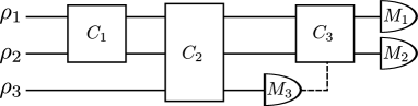
Figure 1: Example of a stabilizer circuit: $\rho_{i}$ have positive representation, $C_{i}$ are Clifford gates and $M_{i}$ have positive representation. The choice of gate $C_{3}$ can be conditioned on the outcome of measurement $M_{3}$.

Notice that there is no loss of generality in considering only symplectic Clifford transformations as the Heisenberg-Weyl component can be rolled into the measurement.

The essential idea for the simulation is to take seriously the hidden variable model the restrictions allow us. In the discrete Wigner picture the system begins at point $\boldsymbol{u}$ in the discrete phase space, which is unknown but definite and fixed. The effect of $U_{\boldsymbol{F}}$ is to move the system from the point $\boldsymbol{u}$ to the point $\boldsymbol{F}\boldsymbol{u}$, and measurement amounts to checking some region of the phase space to see if it contains the system. Since the vector $\boldsymbol{u}$ and matrix $\boldsymbol{F}$ are size $2n$ with entries from $\mathbb{Z}_{d}$ it is computationally efficient to classically store and update the system’s location. Of course, a (positively represented) quantum state corresponds to a probability density over the space so we must treat this a little more carefully. The simulation protocol is:

1. Sample $\boldsymbol{u}\in\mathbb{F}_{d}^{2n}$ according to the distribution $W_{\rho_{1}\otimes\dots\otimes\rho_{n}}(\boldsymbol{u})=W_{\rho_{1}}(\boldsymbol{u}_{1})W_{\rho_{2}}(\boldsymbol{u}_{2})\dots W_{\rho_{n}}(\boldsymbol{u}_{n}).$

2. Repeat until all registers have been measured:

   1. If the unitary $U_{\boldsymbol{F}}$ is applied then update $\boldsymbol{u}\rightarrow\boldsymbol{Fu}$.

   2. If the measurement $M$ with corresponding POVM $\{E_{k}\}$ is made on the last register of the quantum circuit then report outcome $k$ with probability $W_{E_{k}}(\boldsymbol{u}_{m})$ where $\boldsymbol{u}_{m}$ is the ontic position of the last qudit system, defined by $\boldsymbol{u}=\boldsymbol{u}_{1}\oplus\boldsymbol{u}_{2}\dots\oplus\boldsymbol{u}_{m}.$ If the quantum algorithm conditions further steps on the outcome of measurement on this register then condition further steps of the simulation on measurement outcome $k$.

Algorithm Class 2 Classical Simulation Algorithm
Algorithms in this class sample strings of measurement outcomes $\boldsymbol{k}$ according to the distribution $\text{Pr}(K_{\text{class}}=\boldsymbol{k})$

Our claim is that the classical algorithm in Algorithm Class 2 efficiently simulates the corresponding quantum algorithm in Algorithm Class 1. More precisely,

Theorem 1.

An $n$ qudit quantum algorithm belonging to Algorithm Class 1 is simulable by the corresponding $2n$ dit classical algorithm in Algorithm Class 2 in the sense that the distribution of outcomes $\boldsymbol{k}$ is the same for both algorithms, $\text{Pr}(K_{\text{class}}=\boldsymbol{k})=\text{Pr}(K_{\text{quant}}=\boldsymbol{k})$.

Proof.

The input to the classical circuit is a $2n$ dit string and the transformations are all matrices of size $2n$ with entries in $\mathbb{Z}_{d}$ so the $2n$ dit portion of the claim is obvious.

To show that this protocol genuinely simulates the circuit it suffices to show any string of measurement outcomes $\boldsymbol{k}=\left(k_{1}k_{2}\dots k_{n}\right)$ occurs with the same probability for both the original circuit and the simulation. Lets first consider probability distribution $\text{Pr}(k_{n})$ of the outcomes of the first measurement. In the quantum circuit the preparation $\rho_{1}\otimes\dots\otimes\rho_{n}$ is passed to the (possibly identity) gate $U_{\boldsymbol{F}}$ and measurement $M_{n}$ with corresponding POVM $\{E_{k_{n}}\}$ is applied to the $n$th register. The probability of getting outcome $k_{n}$ is then:

$$\text{Pr}_{\text{quant}}(k_{n}) = \text{Tr}(U_{\boldsymbol{F}}\rho_{1}\otimes\dots\otimes\rho_{n}U_{\boldsymbol{F}}^{\dagger}\mathbb{I}\otimes\dots\otimes\mathbb{I}\otimes E_{k_{n}})$$ (1)

$$= \sum_{\boldsymbol{v}\in\mathbb{Z}_{d}^{2n}}W_{U_{\boldsymbol{F}}\rho_{1}\otimes\dots\otimes\rho_{n}U_{\boldsymbol{F}}^{\dagger}}(\boldsymbol{v})W_{\mathbb{I}\otimes\dots\otimes\mathbb{I}\otimes E_{k_{n}}}(\boldsymbol{v})$$

$$= \sum_{\boldsymbol{v}\in\mathbb{Z}_{d}^{2n}}W_{\rho_{1}\otimes\dots\otimes\rho_{n}}(\boldsymbol{F}^{-1}\boldsymbol{v})W_{\mathbb{I}\otimes\dots\otimes\mathbb{I}\otimes E_{k_{n}}}(\boldsymbol{v}).$$

Where we have recast the inner product into the discrete Wigner form for convenience of comparison. We must now establish that the classical circuit has the same distribution.

Classically, if the system is initially at point $\boldsymbol{v}$ on the discrete phase space then probability of getting outcome $k_{n}$ from the simulation circuit is given by:

$$\text{Pr}_{\text{class}}(k_{n}|\boldsymbol{v}\text{ sampled initially}) = \text{Pr}_{\text{class}}(k_{n}|\boldsymbol{Fv}\text{ final location})$$

$$= W_{\mathbb{I}\otimes\dots\otimes\mathbb{I}\otimes E_{k_{n}}}(\boldsymbol{Fv}).$$

Which just says that the system is moved from point $\boldsymbol{v}$ to point $\boldsymbol{Fv}$ and the probability of outcome $k_{n}$ is the probability we see the system when we look at the region of phase space measured by $\boldsymbol{E}_{k_{n}}$, which is $W_{\boldsymbol{E}_{k_{n}}}(\boldsymbol{Fv})$ by definition. The total probability of outcome $k_{n}$ is then:

$$\text{Pr}_{\text{class}}(k_{n}) = \sum_{\boldsymbol{v}\in\mathbb{Z}_{d}^{2n}}\text{Pr}_{\text{class}}(\boldsymbol{k}|\boldsymbol{v}\text{ sampled init.})\text{Pr}(\boldsymbol{v}\text{ sampled init.})$$ (2)

$$= \sum_{\boldsymbol{v}\in\mathbb{Z}_{d}^{2n}}W_{E_{k_{1}}\otimes\dots\otimes E_{k_{n}}}(\boldsymbol{Fv})W_{\rho_{1}\otimes\dots\otimes\rho_{n}}(\boldsymbol{v})$$

$$= \sum_{\boldsymbol{v}\in\mathbb{Z}_{d}^{2n}}W_{E_{k_{1}}\otimes\dots\otimes E_{k_{n}}}(\boldsymbol{v})W_{\rho_{1}\otimes\dots\otimes\rho_{n}}(\boldsymbol{F}^{-1}\boldsymbol{v}).$$

Comparing Algorithm Class (1), the distribution of measurement outcomes on the last register for the quantum circuit, and Algorithm Class (2), the simulated distribution of measurement outcomes on the last register, we see they are the same.

If the quantum algorithm is independent of the measurement outcomes then simply applying the above argument to each register would suffice to complete the proof. However, in general adaptive schemes are possible, such the algorithm illustrated in Figure 1 on page 1 where the final gate applied depends on the outcome of the measurement on the third qudit. Using the assumption that the registers are measured from last to first we can factor the distribution of outcome strings as

$$\text{Pr}(\boldsymbol{k})=\text{Pr}(k_{1}|k_{2}\dots k_{n})\text{Pr}(k_{2}|k_{3}\dots k_{n})\dots\text{Pr}(k_{n-1}|k_{n})\text{Pr}(k_{n}).$$

Since the simulation conditions on measurement outcome in exactly the same way as the original quantum algorithm a simple inductive argument shows that the distribution of outcomes must be the same for the quantum algorithm and its classical simulator. ∎

Corollary 2.

Quantum algorithms belonging to Algorithm Class 1 offer no super linear advantage over classical computation.

Proof.

We have seen that if it is computationally efficient (linear in the number of qudits) to sample from the classical distributions corresponding to the input state and the measurements then such quantum circuits are efficiently simulable. Since we have assumed separability of the input and measurements and the discrete Wigner function factors this efficient sampling is guaranteed. ∎

A couple of remarks are in order. We have restricted ourselves to separable inputs and measurements, but this is not strictly necessary for efficient simulation. Any positively represented preparation or measurement can be accommodated provided it is possible to classically efficiently sample from the corresponding distribution. Since it is exponentially difficult to even write down general quantum states this is rather strong restriction.

Also, notice that our simulation protocol only samples from the output distribution of a circuit whereas the Gottesman-Knill protocol gives the full quantum state output in the case where the input is a pure stabilizer state. It may appear that the present protocol is weaker in this respect. However, the discrete Wigner function of pure stabilizer states are uniformly valued lines on the phase spaceGross (2006) and these are fully specified by only two points. If we are promised the input state to a Clifford circuit is a stabilizer state then we can sample two distinct points from the corresponding distribution and determine where the circuit maps them. These two output points then suffice to fix the line corresponding to the output stabilizer state.

Finally, we note that, in the context of magic state distillation for example, one may increase the size of the input register conditional on measurement outcomes. This can be accounted for in the simulation protocol above by simply increasing the size of the phase space accordingly and sampling from the new additional positive Wigner functions.

III Magic State Distillation

The main significance of the simulation result just established is that for noisy preparation and measurement it is possible to extend the efficient simulation of quantum circuits beyond the purview of the stabilizer formalism. This result is of major theoretical importance, but it also has practical significance. In particular, the simulation scheme addresses the magic state model, which supplements error free stabilizer resources with high fidelity additional gates produced through the consumption of non-stabilizer ancillas. Recall that the backbone of this process is a distillation protocol that uses stabilizer resources applied to a large number of ancilla input states to produce a few highly pure non-stabilizer states. An immediate corollary of our simulation protocol is that states with positive discrete Wigner representation are not useful for computational speedup in the magic state model. Since this includes a large class of states outside the stabilizer formalism this offers a resolution to the long standing open problem of whether all non-stabilizer states promote stabilizer computation to universal quantum computationBravyi and Kitaev (2005).

The class of algorithms in the previous section encompass a large variety of magic state distillation protocols, but it is still conceptually unclear why states with positive discrete Wigner representation are not useful for magic state distillation. This is especially true since we typically think of the outcome of a magic state distillation routine as a quantum state, rather than a string of measurement outcomes as in the simulation protocol. If we did keep track of the full input distribution then we would be able to use it to reconstruct the quantum state output of a distillation procedure; unfortunately this is impossible to do efficiently, but a little thought shows it is not actually necessary. We do not need to know the final quantum state, we only need to know that it is not helpful for doing quantum computation. The simulation protocol makes it clear that if the quantum state that is put into the circuit has a Wigner function that is a genuine probability distribution then the quantum state that is output (which we measure) must also correspond to a genuine probability distribution. Inspired by this observation, and in view of the great importance of magic state protocols, we devote this section to a direct proof that negative discrete Wigner representation of the ancilla resource states is necessary for such states to be distillable (using stabilizer resources) to a non-stabilizer state of arbitrary purity.

The essential insight of the proof used here is that negative discrete Wigner representation is a resource that can not be created using stabilizer operations; if the input states to a distillation protocol has no negativity in its discrete Wigner representation then the output will not either. This resource character is one of the major insights of the present work. Beyond its conceptual value the alternative proof presented below also closes several loopholes and alternative models not addressed by the simulation protocol, which we discuss at the end of the section.

Conventional magic state protocols perform a Clifford unitary on the input state $\rho_{\text{in}}^{\otimes n}\in L(\mathbb{C}_{d}\otimes\mathbb{C}_{d}^{n-1})$ and make a computational basis measurement on the final $n-1$ qudits, post selecting on the $\left|0\right\rangle$ outcome. This outputs the state,

$$\rho_{\text{out}}=\frac{\text{Tr}_{\mathbb{C}_{d}^{n-1}}\left(\mathbb{I}\otimes|0\rangle\!\langle 0|^{\otimes n}U\rho_{\text{in}}^{\otimes n}U^{\dagger}\mathbb{I}\otimes|0\rangle\!\langle 0|^{\otimes n}\right)}{\text{Normalization}},$$

where the partial trace knocks out the ancilla systems and the normalization in the denominator just guarantees $\text{Tr}(\rho_{\text{out}})=1$. We examine significantly more general protocols: instead of requiring $n$ copies of a qudit input state we allow an arbitrary positively represented input state, in place of a Clifford unitary we allow any completely positive map which preserves the set of positively represented states and in place of the computational basis measurement we allow any positively represented projective measurement. Since positive representation is convex this suffices to eliminate classical randomness as a potential loophole. It also precludes choices of entangled stabilizer measurements as these are still positively represented. For convenience of presentation we define,

$$F(\rho) = \text{min}_{\boldsymbol{u}}\text{Tr}(A_{\boldsymbol{u}}\rho),$$

which is the maximally negative point of the quasi-probability representation of $\rho$ over the phase space. If the input state to a distillation routine is positively represented (ie. $F(\rho)\geq 0$) then its output is also positively represented:

Theorem 3.

Let $\rho_{\text{in}}$ be a density operator on a $n$ qudit Hilbert space such that $F(\rho_{\text{in}})\geq 0$. Let $\Lambda$ be a (completely positive) map on this space for which $F(\rho)\geq 0\implies F(\Lambda(\rho))\geq 0$. Let $P$ be a positively represented projector on this space. If $\rho_{\text{out}}$ is produced by acting on $\rho_{\text{in}}$ with $\Lambda$ and post selecting a measurement on the last $n-1$ qudits on outcome $P$ then $F(\rho_{\text{out}})\geq 0$.

Proof.

Since we can use Heisenberg-Weyl operations to cycle between phase point operations, without loss of generality

$$F(\tilde{\rho}) = \text{min}_{\boldsymbol{u}}\text{Tr}(A_{\boldsymbol{u}}\rho)$$

$$= \frac{\text{Tr}(A_{\boldsymbol{0}}\otimes\mathbb{I}^{\otimes n-1}\cdot\mathbb{I}\otimes P\cdot\Lambda(\rho_{\text{in}})\cdot\mathbb{I}\otimes P)}{\text{Normalization}}$$

$$= \frac{\text{Tr}(A_{\boldsymbol{0}}\otimes P\cdot\Lambda(\rho_{\text{in}}))}{\text{Normalization}}.$$

The denominator is always positive so

$$F(\tilde{\rho})\geq 0\iff\text{Tr}(A_{\boldsymbol{0}}\otimes P\cdot\Lambda(\rho_{\text{in}}))\geq 0.$$

By assumption $F(\rho_{\text{in}})$ is positive, and thus so is $F(\Lambda(\rho_{\text{in}}))$. We write $P=\sum_{\boldsymbol{v}}z_{\boldsymbol{v}}A_{\boldsymbol{v}}$ where, since $P$ is positively represented, $z_{\boldsymbol{u}}\geq 0$ by the discrete Hudson’s theorem. This gives us that,

$$\text{Tr}(A_{\boldsymbol{0}}\otimes P\cdot\Lambda(\rho_{\text{in}}))=\sum_{\boldsymbol{v}}z_{\boldsymbol{v}}\text{Tr}(A_{\boldsymbol{0}}\otimes A_{\boldsymbol{v}}\Lambda(\rho_{\text{in}})).$$

The non-negativity of $F(\Lambda(\rho_{\text{in}}))$ implies, by definition, that $\text{Tr}(A_{\boldsymbol{0}}\otimes A_{\boldsymbol{v}}\Lambda(\rho_{\text{in}}))\geq 0$ so it must be the case that $\text{Tr}(A_{\boldsymbol{0}}\otimes P\cdot\Lambda(\rho_{\text{in}}))\geq 0$ and this implies $F(\tilde{\rho})\geq 0.$ ∎

This proof has a few technical merits over the simulation result of the previous section. Namely, it does not require the input state to the distillation protocol to be separable or otherwise efficiently sampleable and the update dynamics are not limited to only Clifford unitary maps. Indeed it’s not even necessary to have a description of the input state or the transformation, all that is required is the promise that $\Lambda(\rho_{\text{in}})$ has positive discrete Wigner representation. Since many input states and channels do not admit any efficient representation this means that there are resources that are provably useless for distillation even when an efficient simulation of the corresponding distillation process would be impossible.

IV The Geometry of Positively Represented States

The Gottesman-Knill theorem already establishes that the action of (qubit) Clifford unitary operations on stabilizer states is efficiently classically simulatable. Since the only pure states with positive discrete Wigner representation are stabilizer states it is natural to wonder if every positively represented state is a mixture of stabilizer states. As we have already alluded to, remarkably this is false. To establish this we will clarify the geometry of the region of state space which has positive representation and show that it strictly contains the set of mixtures of stabilizer states. Combined with the results of the previous sections this establishes our simulation protocol as an extension of Gottesman-Knill and proves the existence of bound states for magic state distillation, states which are not convex combinations of stabilizer states but which are nevertheless not distillable using perfect Clifford operations.

The set of convex combinations of stabilizer states is a convex polytope with the stabilizer states as vertices. Any polytope can be defined either in terms of its vertices or as a list of half space inequalities called facets. Intuitively, these correspond to the faces of $3$ dimensional polyhedrons. We show that in power of prime dimension each of the $d^{2}$ phase space point operators define a facet of the stabilizer polytope. These are only a proper subset of the faces of the stabilizer polytope, implying the existence of states with positive representation which are not convex combinations of stabilizer states. See Figure 2 for a cartoon capturing the intuition for this result.

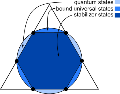
Figure 2: A cartoon of the intersection of the discrete Wigner probability simplex (the triangular region) with the quantum state space (the circle). The simplex intersects the boundary at stabilizer states (bold dots). The region of convex combinations of stabilizer states is strictly contained within the set of quantum states that also lie inside the simplex. The quantum states outside the simplex are the bound states. Finally, the quantum states with negative discrete Wigner representation are those lying outside the positive discrete Wigner simplex. We show that the half space inequalities defining the facets of discrete Wigner simplex also define the facets of the stabilizer polytope; a fact reflected in this cartoon.

The stabilizer polytope may be thought of as a bounded convex polytope living in $\mathbb{R}^{d^{2}-1}$, the space of $d$ dimensional mixed quantum states. A minimal half space description for a polytope in $\mathbb{R}^{D}$ is a finite set of bounding equalities called facets $\{F_{i},f_{i}\}$ with $F_{i}\in\mathbb{R}^{D}$ and $f_{i}\in\mathbb{R}$. $X\in\mathbb{R}^{D}$ is in the polytope if and only if $X\cdot F_{i}\leq f_{i}\ \forall i$. In the usual quantum state space the vectors $X$ of interest are density matrices, the inner product is the trace inner product and facets may be defined as $\{\hat{A}_{i},a_{i}\}$ where $\hat{A}_{i}$ are Hermitian matrices and

$$\rho\in\text{polytope}\iff\text{Tr}(\rho\hat{A}_{i})\leq a_{i}\ \forall i.$$

The objective is to show that $\{-A_{\boldsymbol{u}},0\}$ are facets of the polytope defined by stabilizer state vertices.

It is possible to explicitly compute a facet description for a polytope given the vertex description, but the complexity of this computation scales polynomially in the number of vertices. Since the number of stabilizer states grows super-exponentially with the number of qudits Gross (2006) the conversion is generally impractical. The analytic proof given here circumvents this issue. We also remark that the work of Cormick et al Cormick et al. (2006) implies that the phase space point operators considered here are facets for the case of prime dimension.

Theorem 4.

The $d^{2}$ phase space point operators $\{A_{\boldsymbol{u}}\}$ with the inequalities $\text{Tr}(\rho A_{\boldsymbol{u}})>0$ define facets of the stabilizer polytope.

Proof.

To establish that a halfspace inequality for a polytope in $\mathbb{R}^{D}$ is a facet there are two requirements: every vertex must satisfy the inequality and there must be a set of vertices saturating the inequality which span a space of dimension $D$ Ziegler (1995).

The requirement that all vertices satisfy the half space inequality is $\text{Tr}(A_{\boldsymbol{u}}S)\geq 0$ for every stabilizer state $S$, and this the discrete Hudson’s theorem.

We consider the stabilizer polytope as an object in $\mathbb{R}^{d^{2}-1}$ and look for a set of $d^{2}-1$ linearly independent vertices which satisfy $\text{Tr}(A_{\boldsymbol{u}}S)=0$. Since we are restricting to power of prime dimension we may choose a complete set of mutually unbiased bases of $d(d+1)$ states from the full set of stabilizer states. Suppose more than $d+1$ states $V_{i}$ from this set satisfy $\text{Tr}(V_{i}A_{\boldsymbol{u}})>0.$ Then a counting arguments shows that there must be two distinct states $V_{0},V_{1}$ belonging to an orthonormal basis which satisfy this criterion. But then

$$\text{Tr}(V_{0}V_{1}) =\frac{1}{d}\sum_{\boldsymbol{v}}\text{Tr}(V_{0}A_{\boldsymbol{v}})\text{Tr}(V_{1}A_{\boldsymbol{v}})$$

$$\geq\frac{1}{d}\text{Tr}(V_{0}A_{\boldsymbol{u}})\text{Tr}(V_{1}A_{\boldsymbol{u}})\neq 0,$$

which contradicts the orthonormality. Thus at least $d(d+1)-(d+1)$ states in the mutually unbiased bases satisfy $\text{Tr}(A_{\boldsymbol{u}}V_{i})=0$. These are the required a set of $d^{2}-1$ linearly independent vertices. ∎

The phase space point operators considered here give only a proper subset of the defining halfspace inequalities for the stabilizer polytope. This means that there are states that may not be written as a convex combination of stabilizer states which nevertheless satisfy $\text{Tr}(A_{\boldsymbol{u}}\rho)\geq 0$ for all phase space point operators. That is, there are positive states which are not in the convex hull of stabilizer states. These are bound states for magic state distillation. An explicit example of such a state for the qutrit is given in Gross (2006). These regions can be visualized by taking two and three dimensional slices of the qutrit state space. Such slices are depicted in Figures 3 and 4.

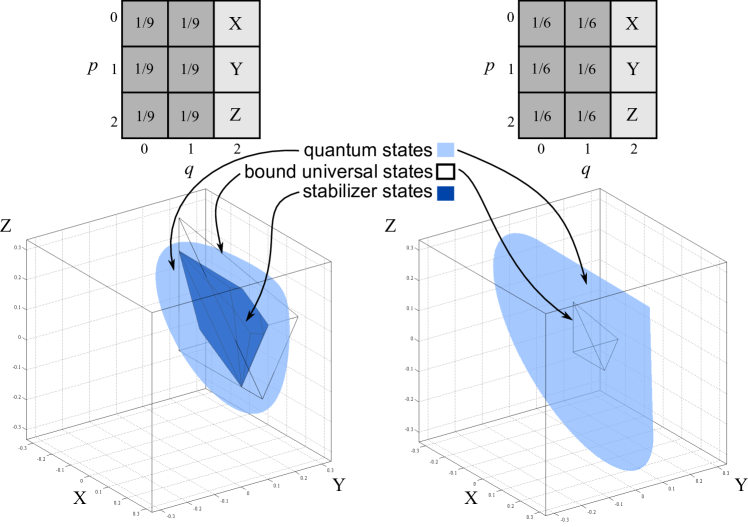
Figure 3: Orthogonal 3-dimensional slices of qutrit state space. Above each slice is the six values of the Wigner function which are fixed at a value of $1/9$ (left) and $1/6$ (right). The remaining three values are allowed to vary and carve out regions depicted in the graphs. In each case, due to symmetries, there are ${9\choose 6}=84$ such slices which are identical (up to a relabeling of the axes). Note that the slice on the right does not cut through the stabilizer polytope but does contain a region of bound states. Also note that this slice contains one of the $9$ states with a maximal negativity of $1/3$ while the slice on the left, and those equivalent up to permutations, are the only ones which feature the maximally mixed state $(X,Y,Z)=1/9$. See also Figure 4 for 2-dimensional slice of the figure on the left.

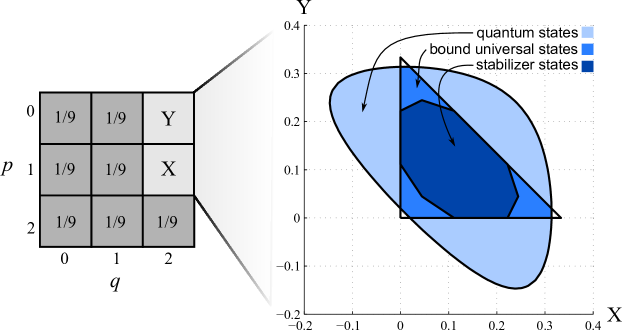
Figure 4: Orthogonal 2-dimensional slice of qutrit state space. On the left are the seven values of the Wigner function which are fixed at a value of $1/9$. The remaining two are allowed to vary. The maximally mixed state is the point $(X,Y)=(1,1)/9$. The various regions carved out by varying these values are shown on the right. There are ${9\choose 7}=36$ such slices which are identical (up to a relabeling of the axes). These would be the only slices featuring the maximally mixed state. Note the remarkable similarity the caricature in 2.

V Discussion and Conclusions

We have shown that for systems of odd power of prime dimension a necessary condition for computational speedup using Clifford unitaries is negativity of the discrete Wigner representation of the inputs. This result is immediately relevant in the context of magic state distillation, where it shows that a necessary condition for distillability is negative representation of the ancilla preparation. We have also shown that the phase space point operators defining the discrete Wigner function correspond to a privileged set of facets of the stabilizer polytope. Together the two results imply the existence of non-stabilizer resources which do not promote Clifford computation to universal quantum computation; and in particular this establishes the existence of bound states for magic state distillation, or bound universal states.

We motivated the development of negative discrete Wigner representation by analogy to entanglement theory, with Clifford operations playing the role of local operations and classical communication and stabilizer states playing the role of separable states. It is known that there are slightly entangled mixed states that can not be consumed by distillation routines to produce highly entangled statesHorodecki et al. (1998). The non-stabilizer but positively represented quantum states are exactly analogous to these bound entangled states. Similarly, it is known that for pure states large amounts of entanglement are required for quantum computational speedupVidal (2003b), but for mixed states this is still an open question. However, for negative discrete Wigner representation there is no relevant distinction between mixed states and pure states. Moreover, although it is not yet known whether every negatively represented state is distillable we conjecture this to be the case.

The discrete Wigner function considered in this work is defined by analogy with the more familiar continuous variable Wigner function. It is natural to wonder if the results of this work extend to the infinite dimensional case. In the continuous case a pure state has positive Wigner representation if and only if it is a Gaussian stateHudson (1974) (like stabilizer states in the discrete case) and a unitary evolution acts as a symplectic flow on the phase space if and only if it corresponds to a quadratic Hamiltonian Weedbrook et al. (2011) (like Clifford gates in the discrete case). A result of Brocker and Werner Bröcker and Werner (1995) shows that there are mixed states that can not be represented as probabilistic combinations of Gaussian states but that nevertheless have positive Wigner function. The natural question is then: is it possible to efficiently simulate quantum systems with quadratic Hamiltonian dynamics acting on non-Gaussian mixed states if these states have positive representation? The answer to this question, yes, is obtained by giving an explicit efficient simulation protocol for such systems Ferrie et al. (In Preparation). This establishes that two of the main results of the present paper (efficient simulation and non-stabilizer mixed states with positive discrete Wigner representation) extend to the continuous case. It is interesting to ask if our third result, that negative discrete Wigner representation is a necessary resource for distillation, also has an analogue. That is, does the continuous variable case admit something analogous to the magic state model which allows noisy negatively represented states to be consumed in order to promote linear optics to full universal quantum computational power?

Of course there remains a final detail that we have not yet addressed. The discrete Wigner function underpinning our analysis is only defined for odd dimensional systems; is it possible to find a similar construction for qubits? The discrete Wigner function used here has two crucial properties: Clifford operations are stochastic transformations on the underlying phase space and this phase space is separable. For qubit systems there is no known analogue. Indeed it is easy to see that a quasi-probability representation defined by any proper subset of the facets of the qubit stabilizer polytope in a fashion analogous to what has been done here will assign positive representation to some subset of the magic states. The construction of the discrete Wigner function, and the Clifford group, relies critically on the mathematics of finite fields, and it is well known that fields of characteristic 2 behave fundamentally differently than fields of any other characteristic. This fact is reflected in the theory of error correction where somewhat different protocols are required for dealing with bits and qubits than are used for dits and qudits. In the case of error correction, although qubits require more involved mathematics, the conceptual underpinnings are the same irrespective of the underlying dimensionality of the dits. It is not unreasonable to hope that a similar result will hold for qubits and that an appropriately modified mathematical strategy will preserve the conceptual insights and related technical results obtained in the qudit case. If this turns out not to be the case then understanding exactly why the model fails for qubits will undoubtedly provide deep insights into the workings of quantum theory and quantum computation.

The most interesting outstanding question raised by this work is whether the ability to prepare any state with negative discrete Wigner representation is sufficient to promote Clifford computation to universal quantum computation. In prime dimension the discrete Wigner construction is the unique choice of quasi-probability representation covariant under the action of Clifford operations Gross (2006), where the law of total probability is required to hold. On this basis we conjecture that the condition here is sufficient. From the work of Campbell, Anwar and Browne Campbell et al. (2012) it is already known that access to any non-stabilizer pure state (or equivalently any negatively represented pure state) suffices. If this conjecture is true then this implies an equivlance of two previously unrelated concepts of non-classicality, namely, quantum computational speedup and negative quasi-probability representation.

Acknowledgements - We thank Nathan Weibe, Daniel Gottesman and Ben Reichardt for helpful comments. After completion of this work we became aware of complementary work by Mari and Eisert Eisert and Mari which develops an alternative efficient simulation for systems with positively represented Wigner function in odd and infinite dimenions. We acknowledge financial support from CIFAR, the Government of Canada through NSERC, and the Ontario Government through OGS and ERA. J.E. thanks the Perimeter Institute for Theoretical Physics where this work was brought to completion.

References

- Aaronson and Gottesman [2004] Scott Aaronson and Daniel Gottesman. Improved simulation of stabilizer circuits. Physical Review A, 70(5):052328+, November 2004. doi: 10.1103/PhysRevA.70.052328. URL http://dx.doi.org/10.1103/PhysRevA.70.052328.
- Anwar et al. [2012] Hussain Anwar, Earl T. Campbell, and Dan E. Browne. Qutrit magic state distillation. New Journal of Physics, 14(6):063006+, June 2012. ISSN 1367-2630. doi: 10.1088/1367-2630/14/6/063006. URL http://dx.doi.org/10.1088/1367-2630/14/6/063006.
- Bravyi and Kitaev [2004] Sergei Bravyi and Alexei Kitaev. Universal Quantum Computation with ideal Clifford gates and noisy ancillas. Physical Review A, 71(2):022316+, December 2004. ISSN 1050-2947. doi: 10.1103/PhysRevA.71.022316. URL http://dx.doi.org/10.1103/PhysRevA.71.022316.
- Bravyi and Kitaev [2005] Sergey Bravyi and Alexei Kitaev. Universal quantum computation with ideal clifford gates and noisy ancillas. Phys. Rev. A, 71:022316, Feb 2005. doi: 10.1103/PhysRevA.71.022316. URL http://link.aps.org/doi/10.1103/PhysRevA.71.022316.
- Bröcker and Werner [1995] T. Bröcker and R. F. Werner. Mixed states with positive Wigner functions. Journal of Mathematical Physics, 36(1):62–75, 1995. URL http://scitation.aip.org/getabs/servlet/GetabsServlet?prog=normal&id=JMAPAQ000036000001000062000001&idtype=cvips&gifs=yes.
- Campbell and Browne [2009] Earl Campbell and Dan Browne. On the structure of protocols for magic state distillation. In Andrew Childs and Michele Mosca, editors, Theory of Quantum Computation, Communication, and Cryptography, volume 5906 of Lecture Notes in Computer Science, pages 20–32. Springer Berlin / Heidelberg, 2009. ISBN 978-3-642-10697-2. URL http://dx.doi.org/10.1007/978-3-642-10698-9_3.
- Campbell [2011] Earl T. Campbell. Catalysis and activation of magic states in fault-tolerant architectures. Phys. Rev. A, 83:032317, Mar 2011. doi: 10.1103/PhysRevA.83.032317. URL http://link.aps.org/doi/10.1103/PhysRevA.83.032317.
- Campbell and Browne [2010] Earl T. Campbell and Dan E. Browne. Bound states for magic state distillation in fault-tolerant quantum computation. Phys. Rev. Lett., 104:030503, Jan 2010. doi: 10.1103/PhysRevLett.104.030503. URL http://link.aps.org/doi/10.1103/PhysRevLett.104.030503.
- Campbell et al. [2012] Earl T. Campbell, Hussain Anwar, and Dan E. Browne. Magic state distillation in all prime dimensions using quantum Reed-Muller codes. May 2012. URL http://arxiv.org/abs/1205.3104.
- Chen et al. [2008] Xie Chen, Hyeyoun Chung, Andrew W. Cross, Bei Zeng, and Isaac L. Chuang. Subsystem stabilizer codes cannot have a universal set of transversal gates for even one encoded qudit. Physical Review A, 78:012353+, July 2008. doi: 10.1103/PhysRevA.78.012353. URL http://dx.doi.org/10.1103/PhysRevA.78.012353.
- Cormick et al. [2006] Cecilia Cormick, Ernesto F. Galvão, Daniel Gottesman, Juan P. Paz, and Arthur O. Pittenger. Classicality in discrete Wigner functions. Physical Review A (Atomic, Molecular, and Optical Physics), 73(1):012301+, 2006. doi: 10.1103/PhysRevA.73.012301. URL http://dx.doi.org/10.1103/PhysRevA.73.012301.
- Datta et al. [2005] Animesh Datta, Steven T. Flammia, and Carlton M. Caves. Entanglement and the power of one qubit. Physical Review A, 72(4):042316+, October 2005. doi: 10.1103/PhysRevA.72.042316. URL http://dx.doi.org/10.1103/PhysRevA.72.042316.
- Douçot and Vidal [2002] Benoit Douçot and Julien Vidal. Pairing of Cooper Pairs in a Fully Frustrated Josephson-Junction Chain. Physical Review Letters, 88(22):227005+, May 2002. doi: 10.1103/PhysRevLett.88.227005. URL http://dx.doi.org/10.1103/PhysRevLett.88.227005.
- Eastin and Knill [2009] Bryan Eastin and Emanuel Knill. Restrictions on Transversal Encoded Quantum Gate Sets. Physical Review Letters, 102:110502+, March 2009. doi: 10.1103/PhysRevLett.102.110502. URL http://dx.doi.org/10.1103/PhysRevLett.102.110502.
- [15] J. Eisert and A. Mari.
- Ferrie and Emerson [2008] C. Ferrie and J. Emerson. Frame representations of quantum mechanics and the necessity of negativity in quasi-probability representations. Journal of Physics A: Mathematical and Theoretical, 41:352001, 2008.
- Ferrie et al. [In Preparation] Chris Ferrie, Victor Veitch, Nathan Wiebe, and Joseph Emerson. Generalized Version of the Gottesman-Knill theorem for Continuous-Variables. In Preparation.
- Ferrie [2011] Christopher Ferrie. Quasi-probability representations of quantum theory with applications to quantum information science. Reports on Progress in Physics, 74(11):116001+, November 2011. ISSN 0034-4885. doi: 10.1088/0034-4885/74/11/116001. URL http://arxiv.org/abs/1010.2701.
- Ferrie and Emerson [2009] Christopher Ferrie and Joseph Emerson. Framed Hilbert space: hanging the quasi-probability pictures of quantum theory. New Journal of Physics, 11(6):063040+, 2009. doi: 10.1088/1367-2630/11/6/063040. URL http://dx.doi.org/10.1088/1367-2630/11/6/063040.
- Ferrie et al. [2010] Christopher Ferrie, Ryan Morris, and Joseph Emerson. Necessity of negativity in quantum theory. Physical Review A, 82(4):044103+, October 2010. doi: 10.1103/PhysRevA.82.044103. URL http://dx.doi.org/10.1103/PhysRevA.82.044103.
- Galvão [2005] Ernesto F. Galvão. Discrete Wigner functions and quantum computational speedup. Physical Review A, 71(4):042302+, April 2005. doi: 10.1103/PhysRevA.71.042302. URL http://dx.doi.org/10.1103/PhysRevA.71.042302.
- Gibbons et al. [2004] Kathleen S. Gibbons, Matthew J. Hoffman, and William K. Wootters. Discrete phase space based on finite fields. Physical Review A, 70(6):062101+, December 2004. doi: 10.1103/PhysRevA.70.062101. URL http://dx.doi.org/10.1103/PhysRevA.70.062101.
- Gottesman [1997] Daniel Gottesman. Stabilizer Codes and Quantum Error Correction. PhD thesis, California Institute of Technology, May 1997. URL http://arxiv.org/abs/quant-ph/9705052v1.
- Gottesman [2006] Daniel Gottesman. Quantum Error Correction and Fault-Tolerance, pages 196–201. Elsevier, July 2006. URL http://arxiv.org/abs/quant-ph/0507174.
- Gross [2006] D. Gross. Hudson’s theorem for finite-dimensional quantum systems. Journal of Mathematical Physics, 47(12):122107+, 2006. URL http://scitation.aip.org/getabs/servlet/GetabsServlet?prog=normal&id=JMAPAQ000047000012122107000001&idtype=cvips&gifs=yes.
- Gross [2007] D. Gross. Non-negative Wigner functions in prime dimensions. Applied Physics B, 86(3):367–370, February 2007. ISSN 0946-2171. doi: 10.1007/s00340-006-2510-9. URL http://arxiv.org/abs/quant-ph/0702004.
- Gross et al. [2007] D. Gross, K. Audenaert, and J. Eisert. Evenly distributed unitaries: On the structure of unitary designs. Journal of Mathematical Physics, 48(5):052104+, 2007. doi: 10.1063/1.2716992. URL http://dx.doi.org/10.1063/1.2716992.
- Horodecki et al. [1998] Michał Horodecki, Paweł Horodecki, and Ryszard Horodecki. Mixed-state entanglement and distillation: Is there a “bound” entanglement in nature? Phys. Rev. Lett., 80:5239–5242, Jun 1998. doi: 10.1103/PhysRevLett.80.5239. URL http://link.aps.org/doi/10.1103/PhysRevLett.80.5239.
- Hudson [1974] R. Hudson. When is the wigner quasi-probability density non-negative? Reports on Mathematical Physics, 6(2):249–252, October 1974. ISSN 00344877. doi: 10.1016/0034-4877(74)90007-X. URL http://dx.doi.org/10.1016/0034-4877(74)90007-X.
- Kenfack and Życzkowski [2004] Anatole Kenfack and Karol Życzkowski. Negativity of the Wigner function as an indicator of non-classicality. Journal of Optics B: Quantum and Semiclassical Optics, 6(10):396+, October 2004. ISSN 1464-4266. doi: 10.1088/1464-4266/6/10/003. URL http://dx.doi.org/10.1088/1464-4266/6/10/003.
- Knill and Laflamme [1998] E. Knill and R. Laflamme. Power of One Bit of Quantum Information. Physical Review Letters, 81(25):5672–5675, December 1998. doi: 10.1103/PhysRevLett.81.5672. URL http://dx.doi.org/10.1103/PhysRevLett.81.5672.
- Lloyd [2002] Seth Lloyd. Quantum Computation with Abelian Anyons. Quantum Information Processing, 1(1):13–18, April 2002. ISSN 15700755. doi: 10.1023/A:1019649101654. URL http://dx.doi.org/10.1023/A:1019649101654.
- Mandel [1986] L. Mandel. Non-Classical States of the Electromagnetic Field. Physica Scripta, 1986(T12):34+, January 1986. ISSN 0031-8949. doi: 10.1088/0031-8949/1986/T12/005. URL http://dx.doi.org/10.1088/0031-8949/1986/T12/005.
- Moore and Read [1991] Gregory Moore and Nicholas Read. Nonabelions in the fractional quantum hall effect. Nuclear Physics B, 360(2-3):362–396, August 1991. ISSN 05503213. doi: 10.1016/0550-3213(91)90407-O. URL http://dx.doi.org/10.1016/0550-3213(91)90407-O.
- N. Ratanje [2011] S. Virmani N. Ratanje. Generalised state spaces and non-locality in fault tolerant quantum computing schemes. January 2011. URL http://arxiv.org/abs/1007.3455v2.
- Reichardt [2005] Ben W. Reichardt. Quantum Universality from Magic States Distillation Applied to CSS Codes. Quantum Information Processing, 4(3):251–264, August 2005. ISSN 1570-0755. doi: 10.1007/s11128-005-7654-8. URL http://dx.doi.org/10.1007/s11128-005-7654-8.
- Reichardt [2009a] Ben W. Reichardt. Error-Detection-Based Quantum Fault-Tolerance Threshold. Algorithmica, 55(3):517–556, November 2009a. ISSN 0178-4617. doi: 10.1007/s00453-007-9069-7. URL http://dx.doi.org/10.1007/s00453-007-9069-7.
- Reichardt [2009b] Ben W. Reichardt. Quantum universality by state distillation. Quantum Information & Computation, 9:1030–1052, July 2009b. URL http://arxiv.org/abs/quant-ph/0608085.
- Schack and Caves [1999] Rüdiger Schack and Carlton M. Caves. Classical model for bulk-ensemble NMR quantum computation. Physical Review A, 60(6):4354–4362, December 1999. doi: 10.1103/PhysRevA.60.4354. URL http://dx.doi.org/10.1103/PhysRevA.60.4354.
- Spekkens [2008] R.W. Spekkens. Phys. Rev. Lett., 101:020401, 2008.
- van Dam and Howard [2009] Wim van Dam and Mark Howard. Tight noise thresholds for quantum computation with perfect stabilizer operations. Phys. Rev. Lett., 103:170504, Oct 2009. doi: 10.1103/PhysRevLett.103.170504. URL http://link.aps.org/doi/10.1103/PhysRevLett.103.170504.
- van Dam and Howard [2011] Wim van Dam and Mark Howard. Noise thresholds for higher-dimensional systems using the discrete wigner function. Phys. Rev. A, 83:032310, Mar 2011. doi: 10.1103/PhysRevA.83.032310. URL http://link.aps.org/doi/10.1103/PhysRevA.83.032310.
- Vidal [2003a] Guifré Vidal. Efficient Classical Simulation of Slightly Entangled Quantum Computations. Physical Review Letters, 91:147902+, October 2003a. doi: 10.1103/PhysRevLett.91.147902. URL http://dx.doi.org/10.1103/PhysRevLett.91.147902.
- Vidal [2003b] Guifré Vidal. Efficient classical simulation of slightly entangled quantum computations. Phys. Rev. Lett., 91:147902, Oct 2003b. doi: 10.1103/PhysRevLett.91.147902. URL http://link.aps.org/doi/10.1103/PhysRevLett.91.147902.
- Wallman and Bartlett [2012] Joel Wallman and Stephen Bartlett. Non-negative subtheories and quasiprobability representations of qubits. Physical Review A, 85(6), June 2012. ISSN 1094-1622. doi: 10.1103/PhysRevA.85.062121. URL http://dx.doi.org/10.1103/PhysRevA.85.062121.
- Weedbrook et al. [2011] Christian Weedbrook, Stefano Pirandola, Raul Garcia-Patron, Nicolas J. Cerf, Timothy C. Ralph, Jeffrey H. Shapiro, and Seth Lloyd. Gaussian Quantum Information. October 2011. URL http://arxiv.org/abs/1110.3234.
- Zeng et al. [2007] Bei Zeng, Andrew Cross, and Isaac L. Chuang. Transversality versus Universality for Additive Quantum Codes, September 2007. URL http://arxiv.org/abs/arXiv:0706.1382.
- Ziegler [1995] Günter M. Ziegler. Lectures on Polytopes. Springer, 1995. ISBN 038794365X, 9780387943657. URL http://books.google.ca/books/about/Lectures_on_Polytopes.html?id=xd25TXSSUcgC&redir_esc=y.