Damped bead on a rotating circular hoop - a bifurcation zoo

Abstract

The evergreen problem of a bead on a rotating hoop shows a multitude of bifurcations when the bead moves with friction. This motion is studied for different values of the damping coefficient and rotational speeds of the hoop. Phase portraits and trajectories corresponding to all different modes of motion of the bead are presented. They illustrate the rich dynamics associated with this simple system. For some range of values of the damping coefficient and rotational speeds of the hoop, linear stability analysis of the equilibrium points is inadequate to classify their nature. A technique involving transformation of coordinates and order of magnitude arguments is presented to examine such cases. This may provide a general framework to investigate other complex systems.

I Introduction

The motion of a bead on a rotating circular hoopgoldstein shows several classes of fixed points and bifurcationsjordansmith ; strogatz ; marsdenratiu . It also exhibits reversibility, symmetry breaking, critical slowing down, homoclinic and heteroclinic orbits and trapping regions. It has been shown to provide a mechanical analogue of phase transitionsfletcher . It can also operate as a one-dimensional ponderomotive particle trapjohnrab . The rigid pendulum, with many applications, can be considered a special case of this systembutikov1 ; butikov2 .

In this article we examine the motion of a damped bead on a rotating circular hoop. Damping alters the nature of the fixed points of the system, showing rich nonlinear features. The overdamped case of this modelstrogatz ; mancuso and a variant involving dry frictionburov has been previously studied.

For certain values of the damping coefficient and the rotational speed of the hoop, linear stability analysis predicts a line of fixed points and some of the fixed points appear as degenerate nodes. However, such fixed points are borderline cases, sensitive to nonlinear terms. By transforming to polar coordinates and employing order of magnitude arguments we analyze these borderline cases to determine the exact nature of these fixed points. To our knowledge, such analytical treatment does not appear in literature. The basic equations obtained for this system are quite generic and arise in other systems (e.g. electrical systems) as well. Hence, our technique may serve as a framework for investigating other more complex nonlinear systems.

II The physical system

A bead of mass $m$, moves on a circular hoop of radius $a$. The hoop rotates about its vertical diameter with a constant angular velocity $\omega$. The position of the bead on the hoop is given by angle $\theta$, measured from the vertically downward direction ($-z$ axis), and $\phi$ is the angular displacement of the hoop from its initial position on the $x$-axis (Figure 1).

Figure 1: Schematic figure of a bead sliding on a rotating hoop showing the angles $\theta$ and $\phi$.

The Lagrangian of the system with no damping is,

$$L(\theta,\dot{\theta})=\frac{ma^{2}}{2}(\dot{\theta}^{2}+\omega^{2}\sin^{2}\theta)+mga\cos\theta\;,\;\;\mbox{where}\;\omega=\dot{\phi}\;\mbox{is a constant}.$$ (1)

Using the Euler-Lagrange equation, the equation of motion is obtained as,

$$\ddot{\theta}=\sin{\theta}(\omega^{2}\cos\theta-g/a).$$ (2)

To include friction, a term $-b\dot{\theta}$ is introduced in (2) as,

$$\ddot{\theta}=\sin{\theta}(\omega^{2}\cos\theta-g/a)-b\dot{\theta}\;,$$ (3)

where $b$ is the damping coefficient. We identify $\omega^{2}_{c}=g/a$ as the critical speed of rotation of the hoop, and write $k=\omega^{2}/\omega^{2}_{c}$, $\mu=b/\omega_{c}$. Defining $\tau=\omega_{c}\;t$, (3) may be made dimensionless by changing from $t$ to $\tau$,

$${\theta}^{{}^{\prime\prime}}=\sin{\theta}(k\cos\theta-1)-\mu\theta^{{}^{\prime}},\;\;\mbox{where}\;\frac{d^{2}\theta}{d\tau^{2}}={\theta}^{{}^{\prime\prime}}\;.$$ (4)

For phase plane analysis, we define a new variable $\theta_{1}=\theta^{{}^{\prime}}$, and write (4) as,

$$\theta^{{}^{\prime}} = \theta_{1}\hskip 125.19194pt$$ (5)

$$\theta_{1}{{}^{\prime}} = -\sin\theta(1-k\cos\theta)-\mu\;\theta_{1}\;.$$ (6)

The parameter $k$ can take only positive values whereas $\mu$ may be either positive or negative.

Due to the symmetry of the hoop about its vertical axis, (5) and (6) remain invariant under the transformations $\theta\to-\theta\;,\;\theta_{1}\to-\theta_{1}$. This implies that alternate quadrants of the $\theta-\theta_{1}$ plane have similar trajectories. Similarly, it is easily verified that if ($\theta(t),\theta_{1}(t)$) is a solution for positive damping ($\mu>0$), then for negative damping ($\mu<0$), ($\theta(-t),-\theta_{1}(-t)$) and ($-\theta(-t),\theta_{1}(-t)$) are two solutions. The phase portrait of the system for negative damping will just be the reflection of the positive damping phase portrait with the arrows reversed. Hence we confine our attention to $\theta\in[0,\pi]$ and $\mu>0$.

When there is no dampingshovan1 , the fixed points are at $(0,0)$ and $(\pi,0)$ for $0\leq k\leq 1$, whereas for $k>1$, an additional fixed point appears at $(\Omega_{1}=\cos^{-1}(1/k),0)$. Damping changes the nature of fixed points and not their number or location.

III Nature of the fixed point $(0,0)$

The Jacobian matrix at $(0,0)$ is obtained by Taylor expanding (5) and (6) about $(0,0)$ and retaining the linear terms.

$$\mathbf{J}(0,0)=\left(\begin{array}[]{ccc}0&1&\\ k-1&-\mu\end{array}\right)\;.$$ (7)

Let $\Gamma$ and $\Delta$ denote the trace and determinant of the above matrix.

1. When $k>1$, both $\Gamma$ and $\Delta$ are negative. The fixed point is a saddle with eigenvalues and eigenvectors given by,

   $$\lambda_{1,2}=\frac{-\mu\pm\xi_{1}}{2},\;\;\;\mathbf{v}_{1,2}=\left(\begin{array}[]{c}1\\ (-\mu\pm\xi_{1})/2\end{array}\right)\;,$$ (8)

   where $\xi_{1}=\sqrt{\mu^{2}+4(k-1)}$. Saddles are robust and do not get perturbed by nonlinearities. Thus, $(0,0)$ will remain a saddle even if nonlinear terms are taken into account (see Figures 8, 9 and 16).

   For $\mu=0$, both $\lambda_{1}$ and $\lambda_{2}$ equal $\sqrt{k-1}$. As $k\to 1^{+}$, $\lambda_{1}\to 0^{+}$ and $\lambda_{2}\to-\mu^{-}$, which means that the saddle will start looking like a line of fixed points along the direction of $\mathbf{v}_{1}$ with solutions decaying along $\mathbf{v}_{2}$.

2. For $0\leq k<1$, $\Gamma=-\mu$ is negative, whereas $\Delta=1-k$ is positive. When there is no damping, the point $(0,0)$ is a center. As $\mu$ is increased, the center transforms into a stable spiral for $\mu<2\sqrt{1-k}$ as shown in Figure 2(a). The frequency of spiralling is $\nu\approx\sqrt{1-k-\mu^{2}/4}$. As $\mu\to 2\sqrt{1-k}^{-}$, $\nu\to 0^{+}$. For $\mu>2\sqrt{1-k}$, the fixed point $(0,0)$ transforms to a stable node (Figure 2(b)). For $\mu=2\sqrt{1-k}$, it is a degenerate node. However, degenerate nodes are borderline cases and are sensitive to nonlinear terms.

3. For $k=1$, (5) and (6) simplify to,

   $$\theta^{{}^{\prime}}=\theta_{1}\hskip 119.50148pt$$ (9)

   $$\theta_{1}^{{}^{\prime}}=-\sin\theta(1-\cos\theta)-\mu\;\theta_{1}\;.$$ (10)

   In the linearized dynamics, $\theta_{1}$ decays exponentially as $e^{-\mu\,t}$. In the phase plane, all trajectories move along a straight line with slope $-\mu$ and stop on reaching the $\theta$ axis. However, the inclusion of nonlinear terms changes this situation.

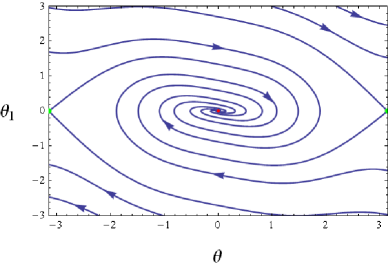
(a)  stable spiral, $\,\mu<2\sqrt{1-k}$

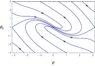
(b)   stable node, $\mu>2\sqrt{1-k}$

Figure 2: Phase trajectories around $(0,0)$ for $k=0.91$ showing (a) stable spiral for $\mu=0.3$ and (b) stable node for $\mu=1$.

III.1 Nature of $(0,0)$ with nonlinearities

1. $\mathbf{0\leq k<1}$ and $\mathbf{\mu<2\sqrt{1-k}}$ :

To include the effect of nonlinear terms, let us define two new variables,

$$\theta=r\cos\phi,\;\;\;\theta_{1}=r\sin\phi$$ (11)

Equations (5) and (6) then may be written as,

$$r^{{}^{\prime}}=r[\cos\phi\sin\phi-2\sqrt{1-k}\sin^{2}\phi]-\sin\phi\sin(r\cos\phi)[1-k\cos(r\cos\phi)]$$ (12)

$$\phi^{{}^{\prime}}=-\sqrt{1-k}\sin(2\phi)-\sin^{2}\phi-\frac{\cos\phi}{r}\sin(r\cos\phi)[1-k\cos(r\cos\phi)]\hskip 22.76228pt$$ (13)

We wish to examine the fixed point(s) in the $r-\phi$ plane corresponding to $(0,0)$ in the $\theta-\theta_{1}$ plane, to determine their true nature. Strictly speaking, (12) and (13) are meaningful only when $r>0$. Neither $\phi$ nor $\phi^{{}^{\prime}}$ have any meaning when $r=0$. Hence, we may assign any arbitrary function $f(\phi)$ to $\phi^{{}^{\prime}}$ at $r=0$ without altering physical predictions. However, (13) describes accurately the approach to $r=0$ (if any) in the $r-\phi$ plane at arbitrarily small scales. We therefore set $f(\phi)$ equal to the limiting value of $\phi^{{}^{\prime}}$ as $r\to 0$.

$$f(\phi)=\lim_{r\rightarrow 0}\phi^{{}^{\prime}}=-\sqrt{1-k}\sin(2\phi)+\frac{k}{2}\cos(2\phi)-\big{(}1-\frac{k}{2}\big{)}$$ (14)

Equations (12) and (13) are periodic in $\phi$ with period $\pi$. Hence, the phase portrait in the $r-\phi$ plane is periodic along the $\phi$-axis with period $\pi$. This means that in the $\theta-\theta_{1}$ plane, the phase space is symmetric about $(0,0)$.

Using the identity $(\sqrt{1-k})^{2}+(k/2)^{2}=(1-k/2)^{2}$, one can write $f(\phi)$ in the form,

$$f(\phi)=\left(1-\frac{k}{2}\right)[\cos(2\phi+\alpha)-1]\;,$$ (15)

where $\alpha=2\tan^{-1}\sqrt{1-k}$, $n=0,1,2,\dots$. Therefore, fixed points $(0,\phi^{*})$ in the $r-\phi$ plane, where $f(\phi^{*})=0$, are given by $\phi^{*}_{n}=n\pi-\tan^{-1}\sqrt{1-k}$ with $n=0,1,2,\dots$. These correspond to the point $(0,0)$ in the $\theta-\theta_{1}$ plane.

The fixed points $(0,\phi^{*}_{n})$ in the $r-\phi$ plane are separated by $n\pi$ (where $n$ is any integer). Hence, in the $\theta-\theta_{1}$ plane, there are no trajectories that can approach $(0,0)$ along two independent directions. So we can say that $(0,0)$ in the $\theta-\theta_{1}$ plane cannot be a stable node. In the $r-\phi$ plane, close to some fixed point $(0,\phi_{n}^{*})$, if there exist trajectories that approach this point and stop there, the corresponding fixed point $(0,0)$ in the $\theta-\theta_{1}$ plane cannot be a stable spiral. For a spiral, $\phi\to\pm\infty$ as $r\to 0$. As (12) and (13) are periodic in $\phi$ with period $\pi$, the nature of all fixed points on the $\phi$-axis separated by $\pi$ is identical. So we may choose to investigate $(0,\phi^{*}=-\tan^{-1}\sqrt{1-k})$. Linearization about this point incorrectly predicts the whole $\phi$ axis to be a line of fixed points. So, we must include the effects of the nonlinear terms. Let $\epsilon=\phi-\phi^{*}$. For small $r$, we may write (12) and (13) as,

$$r^{{}^{\prime}} = -r\Big{[}\sqrt{1-k}-\big{(}1-\frac{k}{2}\big{)}\sin(2\epsilon)\Big{]}+O(r^{3})$$ (16)

$$\epsilon^{{}^{\prime}} = -\left(1-\frac{k}{2}\right)[1-\cos(2\epsilon)]+O(r^{2})\hskip 45.52458pt$$ (17)

Consider an initial condition, $r(\tau=0)=r_{0}$ and $\epsilon(\tau=0)=\epsilon_{0}$, where $0<\epsilon_{0}<\tan^{-1}(\sqrt{1-k}/2)$. For any finite positive value of $1-k$, $\epsilon_{0}$ is finite and $<1/2$. Therefore, $r_{0}$ may be chosen sufficiently small, $0<r_{0}\ll\epsilon_{0}$, so as to make all terms of $O(r^{2})$ and higher, negligible compared to the leading terms in (16) and (17). When these terms are neglected, (16) and (17) may be solved to yield,

$$\epsilon(\tau) = \tan^{-1}\Big{[}\frac{1}{(2-k)\tau+\cot\epsilon_{0}}\Big{]}\hskip 119.50148pt$$ (18)

$$r(\tau) = r_{0}\sin\epsilon_{0}\sqrt{[(2-k)\tau+\cot\epsilon_{0}]^{2}+1}\hskip 2.84544pt\exp(-\sqrt{1-k}\;\tau)$$ (19)

According to this solution, the trajectory monotonically approaches the point $(0,0)$ in the $r-\epsilon$ plane as $\tau\to\infty$. This behaviour will hold even with inclusion of nonlinear terms, provided, the terms independent of $r$ and of $O(r)$ remain dominant over the entire trajectory. The following arguments establish that it is indeed so.

First, the trajectory cannot reach the $\phi$ axis at a positive value of $\epsilon$. This is because on the $\phi$ axis, $r^{\prime}=0$ and $\phi^{{}^{\prime}}=f(\phi)<0$ in between two fixed points. Thus, there is already a trajectory running along the $\phi$ axis directed towards $\epsilon=0$.

For the initial point $(r_{0},\epsilon_{0})$, with the choice $0<r_{0}\ll\epsilon_{0}<1/2$, both $r$ and $\epsilon$ will start to decrease as per (16) and (17). Hence $r^{2}$ will become more negligible compared to $r$. Also, for all $0\leq\epsilon\leq\epsilon_{0}$, the $\epsilon$ independent term, namely, $-\sqrt{1-k}\,r$, in (16), will be dominant. However, if $\epsilon$ decays more rapidly, such that at some stage $r\sim\epsilon$, then the $O(r^{2})$ term will contribute on the same scale as the first term in (17), which is $O(\epsilon^{2})$. Similarly, the $O(r^{3})$ term will contribute on the same scale as the 2nd term in (16) if in the course of decay, at some point $\epsilon\sim r^{2}$. However, such situations will never arise as is shown below.

Let us assume that $r_{0}=\epsilon_{0}^{20}\ll 1$ and that $\epsilon$ decreases very rapidly, such that, at some instance, $r=\epsilon^{2}$. As $r$ has decreased monotonically from its initial value, we must have $\epsilon=r^{1/2}<r_{0}^{1/2}$. However, $r_{0}^{1/2}=\epsilon_{0}^{10}\ll 1$. Hence, along the entire trajectory, up to this instance, terms of $O(r^{2})$ and higher are negligible compared to the leading terms in (16) and (17). Thus the solutions (18) and (19) are valid and give the correct orders of magnitudes of the dynamical quantities.

As $0<\epsilon<\epsilon_{0}^{10}\ll 1$ and $0<\epsilon_{0}<1/2$, we may write, $\tan\epsilon\sim\epsilon$ and $\tan\epsilon_{0}\sim\epsilon_{0}$. Hence, $0<\tan\epsilon<\tan^{10}\epsilon_{0}$, which implies $\tan\epsilon<(\sqrt{1-k}/2)^{10}\ll 1$. Combining this with (18) and using the fact that $(2-k)\sim 1$, we get $\tau\gtrsim(\cot\epsilon_{0})^{10}$, a very large quantity. Meanwhile (18) and (19) together imply,

$$\frac{r}{\epsilon^{2}}\sim r_{0}\sin\epsilon_{0}\Big{[}\frac{\tau^{3}}{\exp(\sqrt{1-k}\;\tau)}\Big{]}$$ (20)

Both $r_{0}\sin\epsilon_{0}$ and the quantity within brackets are $\ll 1$, which implies that $r\ll\epsilon^{2}$. This is in contradiction to the initial assumption that $r=\epsilon^{2}$. Therefore, we conclude that starting with the prescribed initial condition, $r$ will never become equal to $\epsilon^{2}$. This ensures that along the entire trajectory, the terms independent of $r$ and of $O(r)$ remain the dominant terms in (16) and (17). Both $r$ and $\epsilon$ will decrease monotonously toward their respective zero values. Neither can the trajectory cross the curve $r=\epsilon^{2}$ nor reach the $\phi$ axis before $\epsilon$ becomes zero. Thus, the trajectories in the $r-\epsilon$ plane must approach $(0,0)$ tangential to the $\phi$ axis and slow to a halt there.

In the $\theta-\theta_{1}$ plane, the above arguments imply that, trajectories exist which start at a finite distance from $(0,0)$ and reach this point along a line of slope $-\sqrt{1-k}$. Also, no other such line with a different slope exists. These facts clearly establish that $(0,0)$ is a stable degenerate node (Figure 3).

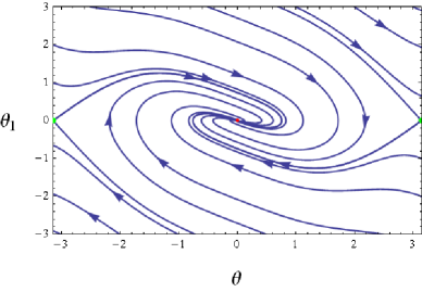
(a)  stable degenerate node, $\mu=0.6$

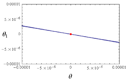
(b)  central region magnified

Figure 3: Phase trajectories around $(0,0)$ for $k=0.91$ and $\mu=2\sqrt{1-k}$.

2. $\mathbf{k=1}$ :

Proceeding as before, (9) and (10) may be written in terms of $r$ and $\phi$ as,

$$r^{{}^{\prime}} = r[\cos\phi\sin\phi-\mu\sin^{2}\phi]-\sin\phi\sin(r\cos\phi)[1-\cos(r\cos\phi)]$$ (21)

$$\phi^{{}^{\prime}} = -\mu\cos\phi\sin\phi-\sin^{2}\phi-\frac{\cos\phi}{r}\sin(r\cos\phi)[1-\cos(r\cos\phi)]$$ (22)

$f(\phi)$ is defined as,

$$f(\phi)=\lim_{r\rightarrow 0}\phi^{{}^{\prime}}=-\mu\cos\phi\sin\phi-\sin^{2}\phi$$ (23)

The phase portrait is periodic in $\phi$ with period $\pi$. The fixed points in the $r-\phi$ plane of the form (0,  $\phi^{*}$) are given by,

$$\phi^{*}_{1}=n\pi\hskip 14.22636pt\mbox{and}\hskip 14.22636pt\phi^{*}_{2}=n\pi-\tan^{-1}\mu\;\;n=0,1,2,\dots.$$ (24)

For $-\tan^{-1}\mu<\phi<0$, $f(\phi)>0$ whereas for $0<\phi<\pi-\tan^{-1}\mu$, $f(\phi)<0$. The positive and negative nature of $f(\phi)$ repeats periodically along the $\phi$ axis.

The Jacobian at the points $(0,n\pi-\tan^{-1}\mu)$ given by,

$$\mathbf{J}(0,\phi_{2})=\left(\begin{array}[]{ccc}-\mu&0&\\ 0&\mu\end{array}\right)$$ (25)

is traceless and has a negative determinant $\Delta=-\mu^{2}$. So, this family of fixed points are saddles having stable manifold along $r$ axis and unstable manifold along $\phi$ axis.

Linear analysis of the family of fixed points $(0,n\pi)$, incorrectly predicts $\phi=n\pi$ to be lines of fixed points. Let us examine the point $(0,0)$ in the $r-\phi$ plane for simplicity. Consider the condition,

$$0\leq|\phi|\leq r\ll min\{1,\mu\}$$ (26)

If (26) holds, then neglecting terms of $O(r^{3})$ and smaller in (21) and (22), we may write,

$$r^{{}^{\prime}} = \phi r+\eta_{1}\hskip 56.9055pt$$ (27)

$$\phi^{{}^{\prime}} = -\mu\phi-\frac{r^{2}}{2}-\phi^{2}+\eta_{2}$$ (28)

where $\eta_{1}\sim\phi^{2}r$ and $\eta_{2}\sim\phi^{3}\;\mbox{or}\;\phi^{2}r^{2}$, whichever is larger. Note that as long as (26) is satisfied, both $\eta_{1}$ and $\eta_{2}$ can at most be of the order of $r^{3}$.

Let us take the initial condition $\phi_{0}=0$ and $0<r_{0}\ll 1$. Then, $\phi^{{}^{\prime}}(t=0)=-r_{0}^{2}/2$ and $r^{{}^{\prime}}(t=0)=0$. Hence, $\phi$ will start decreasing and become negative. As a result, $r^{{}^{\prime}}$ will become negative and remain so until $\phi$ or $r$ vanishes, provided (26) remains true. It is seen that as long as the trajectory is above the curve $\phi=-r^{2}/2\mu$, (26) is satisfied and both $r^{{}^{\prime}}$ and $\phi^{{}^{\prime}}$ are negative. Therefore, the trajectory approaches and eventually crosses this curve, where $\phi^{{}^{\prime}}$ is still negative, being of the order of $\phi^{2}$.

Let us consider the ‘trapping region’ in Figure 4, which shows the phase flow on the curves $\phi=-r$ and $\phi=-r^{2}/2\mu$.

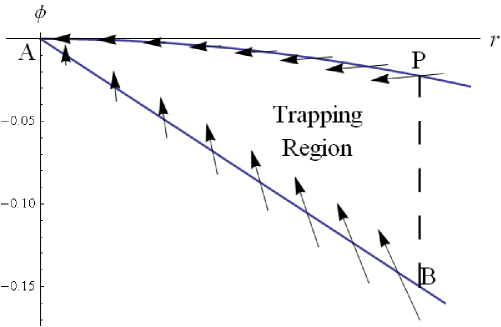
Figure 4: Trapping Region.

At any point on the line $\phi=-r$ for which $r\ll min\{1,\mu\}$,

$$\frac{\phi^{{}^{\prime}}}{r^{{}^{\prime}}}=-\frac{\mu}{r}+O(1)$$

As $r\ll\mu$, $|\phi^{{}^{\prime}}/r^{{}^{\prime}}|\gg 1$. Thus the phase flow is almost vertically upward, as shown in Figure 4. Everywhere inside the region, (26) is satisfied and hence $r^{{}^{\prime}}<0$ and finite. Consequently, after entering the region at point $P$, the trajectory must constantly move towards left. Again, it cannot penetrate the curves $AP$ or $AB$, because other trajectories are actually flowing inward across them. Hence, we have trapped it. Upon arrival at any point on the arc $AP$, a trajectory must inevitably land up at $(0,0)$. Note that at any point on the line $\phi=-mr$, $(0<m\leq 1)$,

$$\frac{\phi^{{}^{\prime}}}{r^{{}^{\prime}}}=-\frac{m\mu-(m^{2}+1/2)r+O(m^{3}r^{2})}{mr+O(m^{2}r^{2})}\;.$$

For any finite value of $m$, this approaches $-\infty$ as $r\to 0$, meaning that the phase flow is almost vertically upward on any line of non-zero slope near $(0,0)$. Therefore, the trajectory must reach $(0,0)$ along the $r$ axis.

Thus, the fixed points $(0,n\pi)$ in the $r-\phi$ plane are stable nodes having slow eigenvector along $r$ axis and fast eigenvector along $\phi$ axis. In between these, lie the saddle points $(0,n\pi-\tan^{-1}\mu$) (Figure 5).

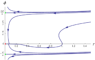
(a)  stable node and saddle points

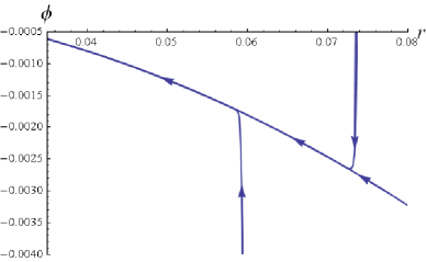
(b)  region near $(0,0)$ magnified

Figure 5: Phase portrait in the $r-\phi$ plane.

These results from the $r-\phi$ plane mean that in the $\theta-\theta_{1}$ plane, two trajectories exist which reach $(0,0)$ along the line of slope $-\mu$ and all other neighbouring trajectories reach it along the $\theta$ axis. In other words, $(0,0)$ is a stable node here.

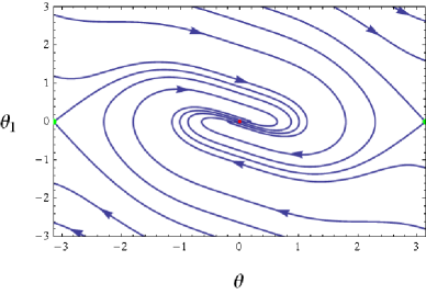
(a)  stable node

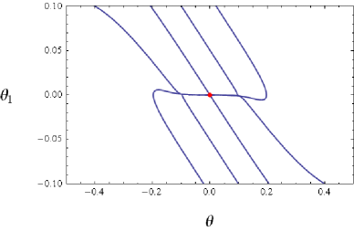
(b)  central region magnified

Figure 6: Phase trajectories about $(0,0)$ in the $\theta-\theta_{1}$ plane for $k=1$ and $\mu=0.5$.

Figure 7a shows the nature of the fixed point at $(0,0)$ over the entire parameter space.

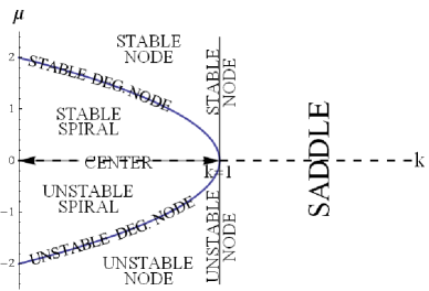
(a)  $(0,0)$, curve is $\mu=2\sqrt{1-k}$

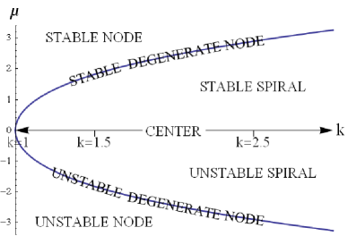
(b)  $(\pm\Omega_{1},0)$, curve is $\mu=2\sqrt{k-1/k}$

Figure 7: Nature of fixed points $(0,0)$ and $(\pm\Omega_{1},0)$ over the $k-\mu$ plane

IV Nature of the fixed point $(\Omega_{1},0)$

This fixed point exists when $k\geq 1$. Linearization of (5) and (6) gives us the Jacobian at $(\Omega_{1},0)$ as,

$$\mathbf{J}(\Omega_{1},0)=\left(\begin{array}[]{ccc}0&1&\\ \left(\frac{1}{k}-k\right)&-\mu\end{array}\right)$$ (29)

For $0\leq\mu<2\sqrt{k-\frac{1}{k}}$, $(\Omega_{1},0)$ is a stable spiral with eigenvalues given by,

$$\lambda=-\frac{\mu}{2}\pm i\sqrt{(k-\frac{1}{k})-\frac{\mu^{2}}{4}}$$

Trajectories spiral in with an angular frequency $\nu\approx\sqrt{(k-1/k)-\mu^{2}/4}$, while their radial distance decreases as $e^{-\mu t/2}$. As $\mu\to 0$, this decay rate vanishes and ($\Omega_{1},0)$ turns into a center (Figure 8). Also, $\nu$ vanishes as $\mu\to 2\sqrt{k-1/k}^{-}$, representing a smooth transition to a stable node, similar to the behaviour of the fixed point $(0,0)$.

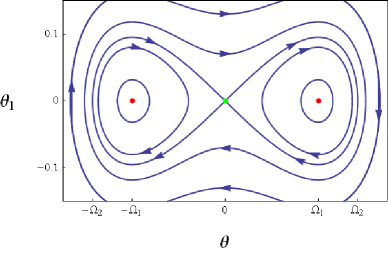
(a)  center, $\mu=0$

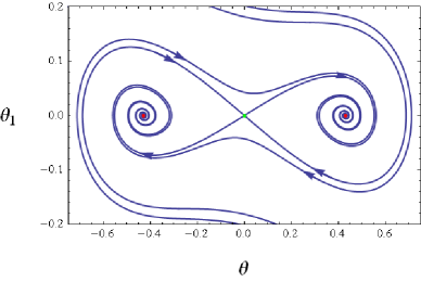
(b)  stable spiral, $\mu=0.1$

Figure 8: Phase trajectories around $(0,0)$ for $k=1.1$ and $0\leq\mu<2\sqrt{k-\frac{1}{k}}$.

When $\mu>2\sqrt{k-\frac{1}{k}}$, $\Gamma^{2}-4\Delta>0$, hence $(\Omega_{1},0)$ is a stable node (Figure 9), with eigenvalues and eigenvectors given by,

$$\lambda_{1,2}=\frac{-\mu\pm\xi_{3}}{2},\;\;\;\mathbf{v}_{1,2}=\left(\begin{array}[]{c}1\\ (-\mu\pm\xi_{3})/2\end{array}\right)\;,$$

where $\xi_{3}=\sqrt{\mu^{2}-4(k-1/k)}$. Both $\lambda_{1}$ and $\lambda_{2}$ approach the value $-\sqrt{k-1/k}$ as $\mu\to 2\sqrt{k-1/k}^{+}$, indicating a stable degenerate node.

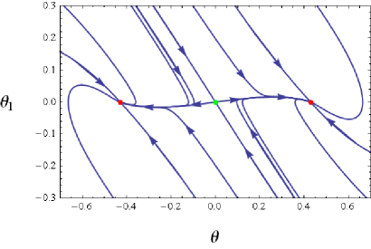
(a)  stable node, $\mu=1$

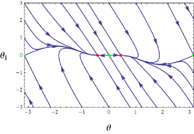
(b)  stable node, $\mu=2.5$

Figure 9: Phase trajectories around $(0,0)$ for $k=1.1$ and $\mu>2\sqrt{k-\frac{1}{k}}$.

For $\mu=2\sqrt{k-\frac{1}{k}}$, $\Gamma^{2}-4\Delta=0$. In the linear stability analysis, $(\Omega_{1},0)$ is a stable degenerate node with a single eigenvector,

$${\mathbf{v}}=\left(\begin{array}[]{c}1\\ -\sqrt{k-1/k}\end{array}\right)\;,$$ (30)

corresponding to the eigenvalue $\lambda=-\sqrt{k-1/k}$. However, degenerate nodes can be transformed into stable nodes or stable spirals due to perturbation introduced by nonlinear terms.

IV.1 Nature of $(\Omega_{1},0)$ with nonlinearities

As discussed in subsection III.1, (5) and (6) may be transformed to equations in $r$ and and $\phi$ with the substitutions, $\theta-\Omega_{1}=r\cos\phi$ and $\theta_{1}=r\sin\phi$. Define,

$$f(\phi)=\lim_{r\to 0}\phi^{{}^{\prime}}=-\sqrt{k-\frac{1}{k}}\sin(2\phi)-\frac{1}{2}(k-\frac{1}{k}-1)\cos(2\phi)-\frac{1}{2}(k-\frac{1}{k}+1)$$ (31)

$f(\phi)$ is negative at all points on the $\phi$ axis except at the fixed points given by $(0,\phi^{*})$ with $\phi^{*}=n\pi-\alpha$, where $\alpha=\tan^{-1}\sqrt{k-1/k}$, ($n=0,1,2,\dots$), where it is zero. These fixed points are separated by $n\pi$. Then, by the same reasoning as used in III.1, we can argue that $(0,0)$ cannot be a stable node. The remaining possibilities are a spiral or a degenerate node.

Let us consider the fixed point $(0,-\alpha)$, and let $\epsilon=\phi+\alpha$. Then we may expand $r^{{}^{\prime}}$ and $\epsilon^{{}^{\prime}}$ upto $O(r)$,

$$r^{{}^{\prime}}=-\frac{1}{2}\Big{(}k-\frac{1}{k}+1\Big{)}\big{(}\sin(2\alpha)-\sin(2\epsilon)\big{)}r+O(r^{2})\hskip 85.35826pt$$ (32)

$$\epsilon^{{}^{\prime}}=-\Big{(}k-\frac{1}{k}+1\Big{)}\sin^{2}\epsilon-\frac{3}{2}r\sqrt{1-\frac{1}{r^{2}}}\cos^{3}\alpha\hskip 108.12054pt$$

$$-\frac{9}{4}\sqrt{1-\frac{1}{k^{2}}}\cos\alpha\;\sin(2\alpha)\;r\;\epsilon+O(r^{2})\hskip 119.50148pt$$ (33)

We choose an initial point, $(r_{0},\epsilon_{0})$, and $0<r_{0}\ll\epsilon_{0}<min\{1,\alpha\}$. This choice ensures that both $r$ and $\epsilon$ will start decreasing. In the course of this monotonic decay, $r$ cannot reach zero before $\epsilon$ becomes zero, as there is a straight line trajectory moving downward along the $\phi$ axis. From (32) and (33) we note that $r^{{}^{\prime}}$ and $\epsilon^{{}^{\prime}}$ each contains an $\epsilon$ independent term of $O(r)$. Therefore, as $r$ and $\epsilon$ decrease toward their respective zero values, the 1st order approximation gets even better. However, if at some stage, $\epsilon\sim r$, then the $O(r^{2})$ terms would contribute on the same scale as some of the terms of $O(r\epsilon)$ in (32) and (33). But the following argument rules out such a possibility.

Let us consider a specific case and choose $r_{0}=\epsilon_{0}^{20}$. If $\epsilon$ is to become $O(r)$, at some stage, we must have $r=\epsilon^{2}$. However, for $r=\epsilon^{2}$, we have

$$r^{{}^{\prime}} = -\sqrt{k-\frac{1}{k}}\epsilon^{2}+O(\epsilon^{3})$$

$$\epsilon^{{}^{\prime}} = -\left[(k-\frac{1}{k}+1)+\frac{3}{2}\frac{\sqrt{1-\frac{1}{k^{2}}}}{(k-\frac{1}{k}+1)^{\frac{3}{2}}}\right]\epsilon^{2}+O(\epsilon^{3})$$

whereas along the curve $r=\epsilon^{2}$, $dr/d\epsilon=2\epsilon$. Therefore, for a given value of $k>1$, we can always select an $\epsilon_{0}$, sufficiently small, for which, at all points on the curve $r=\epsilon^{2}$ contained between $\epsilon=0$ and $\epsilon=\epsilon_{0}$, the ratio $r^{{}^{\prime}}/\epsilon^{{}^{\prime}}>dr/d\epsilon$. This would guarantee that the trajectory cannot penetrate down this curve, which means that $\epsilon$ cannot reach zero before $r$ does. Thus, for a suitable choice of initial conditions, the trajectory must slow to a halt at $(r=0,\epsilon=0)$. In the $\theta-\theta_{1}$ plane, this means that there exist trajectories which start at a finite distance from $(\Omega_{1},0)$ and reach it along the line of slope $-\alpha$. Also, there is no other such line with a different slope. Hence, $(\Omega_{1},0)$ is a stable degenerate node (Figure 10).

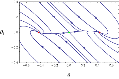
(a)  stable degenerate node

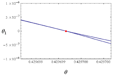
(b)  region around $(\Omega_{1},0)$ magnified

Figure 10: Phase trajectories for $k=1.1$ and $\mu=2\sqrt{k-\frac{1}{k}}$.

Figure 7b gives the nature of the fixed point at $(\pm\Omega_{1},0)$ in different parts of the parameter space.

V Nature of the fixed point $(\pi,0)$

The Jacobian matrix at ($\pi$,0) is given as,

$$\mathbf{J}(\pi,0)=\left(\begin{array}[]{ccc}0&1&\\ k+1&-\mu\end{array}\right)\;.$$ (34)

The fixed point is a saddle for all values of $k$ and remains so even with the inclusion of nonlinear terms. The eigenvalues and corresponding eigenvectors are given by,

$$\lambda_{1,2}=\frac{-\mu\pm\xi_{2}}{2},\;\;\;\mathbf{v}_{1,2}=\left(\begin{array}[]{c}1\\ (-\mu\pm\xi_{2})/2\end{array}\right)\;,\\$$

where $\xi_{2}=\sqrt{\mu^{2}+4(k+1)}$.

V.1 Trajectories

Damping of the bead leads to some qualitatively different trajectories in addition to those observed for the frictionless caseshovan1 . These are mainly the different kinds of damped oscillations (underdamped, critically damped, overdamped) about the stable equilibrium points. Some of these are illustrated with the following numerical plots.

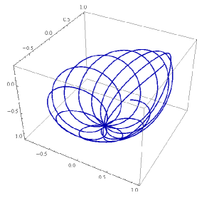
(a)  $k=0.75$, $\mu=0.05$, $\theta^{{}^{\prime}}(0)=0$

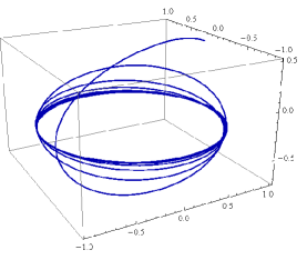
(b)  $k=4$, $\mu=0.5$, $\theta^{{}^{\prime}}(0)=0$

Figure 11: Underdamped oscillation about (a) $\theta=0$ and (b) $\theta=\Omega_{1}$.

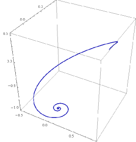
(a)  $k=0.75$, $\mu=1.5$, $\theta^{{}^{\prime}}(0)=0$

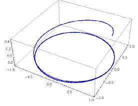
(b)  $k=4$, $\mu=4$, $\theta^{{}^{\prime}}(0)=0$

Figure 12: Overdamped oscillation about (a) $\theta=0$ (b) $\theta=\Omega_{1}$.

VI Phase portraits and Bifurcation

For $0\leq k<1$, the fixed point at $(0,0)$ transforms its nature as the damping coefficient is varied. It is a center at $\mu=0$, as $\mu$ increases, it becomes a stable spiral. At $\mu=2\sqrt{1-k}$, it turns into a stable degenerate node. It makes a smooth transition to a stable node as damping is increased further. Thus, a spiral-node bifurcation takes place at this critical condition (Figures 2 and 3). Physically, as damping is gradually increased from $0$, the system undergoes a continuous transition from undamped oscillations of the bead about $\theta=0$ (center), to underdamped oscillations (stable spiral). At $\mu=2\sqrt{1-k}$, the system is critically damped (degenerate node) and becomes overdamped (stable node) as $\mu$ is increased further.

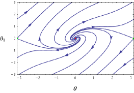
(a)  unstable spiral, $\mu=-1$

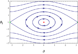
(b)  center, $\mu=0$

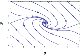
(c)  stable spiral, $\mu=1$

Figure 13: Phase portraits for $k=0$ showing degenerate Hopf bifurcation.

For negative damping, $(0,0)$ becomes an unstable spiral and changes to an unstable node as $\mu$ is made more negative. Consequently, as one crosses $\mu=0$, the fixed point $(0,0)$, undergoes a degenerate Hopf bifurcation (Figure 13).

With increase in the angular speed of the hoop (i.e., $k$), the stability of the origin degrades continuously. When $k=1$, $(0,0)$ is a weak center. A special case of Hopf bifurcation occurs, when $\mu$ is swept from negative to positive values acroos 0, keeping $k$ fixed at 1 (Figure 14).

As $k$ is increased beyond $1$, $(0,0)$ transforms from a stable ($\mu>0$) or unstable ($\mu<0$) node to a saddle. Two new stable nodes appear at $\pm\Omega_{1}=\pm\cos^{-1}(1/k)$ and branch out in opposite directions. Thus, a supercritical pitchfork bifurcation occurs at {$k=1$} (Figure 15a).

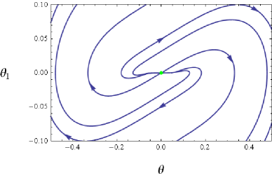
(a)  unstable node, $\mu=-0.2$

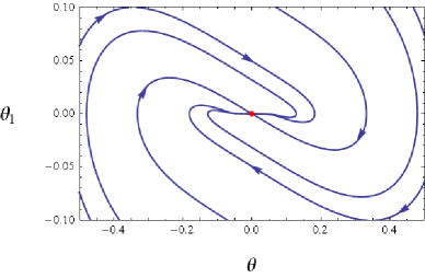
(b)  stable node, $\mu=0.2$

Figure 14: Phase portraits for $k=1$.

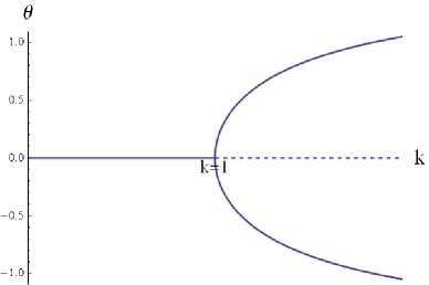
(a)  Supercritical bifurcation at $k=1$, $\mu=0$

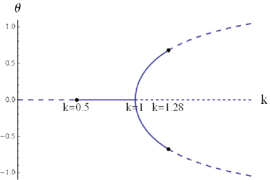
(b)  Supercritical bifurcation at $k=1$, $\mu=\sqrt{2}$

Figure 15: Section of the bifurcation diagram for (a) $\mu=0$ and (b) $\mu>0$. In (a) solid curve represents center, dashed curve represents saddle. In (b) solid curve represents stable node, densely dashed curve represents saddle and sparsely dashed curve represents stable spiral. Supercritical pitchfork bifurcation occurs at $k=1$ and spiral-node bifurcation occurs at $k=0.5$ and $k=1.28$.

As $k$ increases from $1$ to $\infty$, $\Omega_{1}$ varies from $0$ to $\pi/2$. The fixed point $(\Omega_{1},0)$, is a center for zero damping, a stable spiral in the region $0<\mu<2\sqrt{k-1/k}$ (underdamped oscillation), and becomes a stable degenerate node at critical damping $\mu=2\sqrt{k-1/k}$. For the overdamped condition $\mu>2\sqrt{k-1/k}$, it is a stable node.

For negative damping, we get just the unstable counterparts. Accordingly, a spiral-node bifurcation is observed at $\mu=\pm 2\sqrt{k-1/k}$ (Figures 8, 9, 10 and 15)b. A degenerate Hopf bifurcation is observed for $k>1$ and $\mu=0$ (Figure 16).

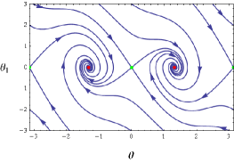
(a)  unstable spiral, $\mu=-1$

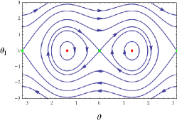
(b)  center, $\mu=0$

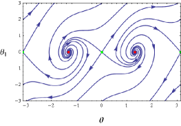
(c)  stable spiral, $\mu=1$

Figure 16: Phase portraits for $k=4$ showing degenerate Hopf bifurcation.

The fixed points $(\pm\pi,0)$ are saddles for all values of $k$. They have saddle connections between them at $\mu=0$, which break in opposite directions for positive and negative damping.

The above observations are summarized in Figure 17 and Table 1 below.

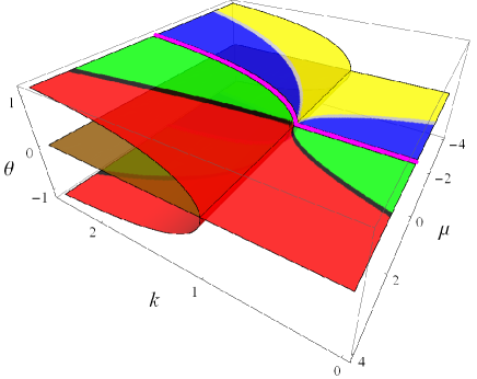
Figure 17: The bifurcation diagram

In Fig 17, red denotes stable node, green denotes stable spiral, blue denotes unstable spiral, yellow denotes unstable node, brown denotes saddle, pink denotes center, gray denotes unstable degenerate node, and black denotes stable degenerate node.

Table 1: Bifurcation Table.

Points in parameter space	Bifurcation along $k$	Bifurcation along $\mu$	Figure references
1) $(k,0)$ ; $k\neq 1$	–	degenerate Hopf	Figures 13, 16
2) $(k,\pm 2\sqrt{1-k})$ ; $0\leq k<1$	spiral-node	spiral-node	Figures 2-3, 15b
3) $(1,0)$	supercritical pitchfork	Hopf	Figures 13b, 8a, 14 , 15a
4) $(1,\mu)$ ; $\mu\neq 0$	supercritical pitchfork	–	Figures 2b, 9a, 14b, 15b
5) $(k,\pm 2\sqrt{k-\frac{1}{k}})$ ; $k>1$	spiral-node	spiral-node	Figures 8-10, 15b

Up to now, we have limited attention to those bifurcations resulting from a variation of k or a variation of $\mu$. From Figure 17, we see that the curves $\mu^{2}=2(1-k)$, $\mu^{2}=2(k-1/k)$, and $k=1$ divide the parameter space into $8$ distinct regions of different dynamics. All these regions meet at the point $\{k=1,\mu=0\}$. Traversing suitable curves in $k-\mu$ space, one can move from any one region to another, yielding new kinds of bifurcation. Following such a curve amounts to keeping a certain function $\alpha(k,\mu)$ constant, while varying some other function $\beta(k,\mu)$. Mathematically, the possibilities are rich. But whether it is possible to actually implement this in the bead-hoop system is subject to further inquiry. However, this would attain physical significance if there exists another system where $\alpha$ and $\beta$ themselves are the control parameters.

Concluding Remarks

The simple introduction of damping to the bead-hoop system enriches its dynamics and leads to various new modes of motion and different classes of bifurcations. We have studied this system over the entire parameter space and presented phase portraits and trajectories. This serves to illustrate the qualitative changes in the system’s dynamics across different bifurcation curves. We have presented exact analytical treatment of the borderline cases where linearization fails, for which no general methods are available in the literature. The method of transforming to polar coordinates and using order of magnitude arguments, employed in this article, can serve as a useful technique for other dynamical systems as well.

References

References

- (1) Goldstein H 1980-07 Classical Mechanics (Addison-Wesley, Cambridge, MA)
- (2) Jordan D W and Smith P 1999 Nonlinear Ordinary Differential Equations : An Introduction to Dynamical Systems (Oxford University Press, New York)
- (3) Strogatz S 2001 Nonlinear Dynamics And Chaos: Applications To Physics, Biology, Chemistry, And Engineering (Addison-Wesley, Reading, MA)
- (4) Marsden J E and Ratiu T S 1999 Introduction to Mechanics and Symmetry (Springer-Verlag, New York)
- (5) Fletcher G 1997 A mechanical analogue of first- and second-order phase transitions Am. J. Phys. 65 74
- (6) Johnson A K and Rabchuk J A 2009 A bead on a hoop rotating about a horizontal axis : A one-dimensional ponderomotive trap Am. J. Phys. 77 1039
- (7) Butikov E I 1999 The rigid pendulum - an antique but evergreen physical model Eur. J. Phys. 20 429
- (8) Butikov E I 2007 Extraordinary oscillations of an ordinary forced pendulum Eur. J. Phys. 29 215
- (9) Mancuso R V 1999 A working model for first- and second-order phase transitions and the cusp catastrophe Am. J. Phys. 68 271
- (10) Burov A A 2009 On bifurcations of relative equilibria of a heavy bead sliding with dry friction on a rotating circle Acta Mechanica 212 349
- (11) Dutta S and Ray S 2011 Bead on a rotating circular hoop: a simple yet feature-rich dynamical system arXiv:1112.4697v1