Estimating parameters of coalescing compact binaries with proposed advanced detector networks
Abstract
The advanced versions of the LIGO and Virgo ground-based gravitational-wave detectors are expected to operate from three sites: Hanford, Livingston, and Cascina. Recent proposals have been made to place a fourth site in Australia or India; and there is the possibility of using the Large Cryogenic Gravitational Wave Telescope in Japan to further extend the network. Using Bayesian parameter-estimation analyses of simulated gravitational-wave signals from a range of coalescing-binary locations and orientations at fixed distance or signal-to-noise ratio, we study the improvement in parameter estimation for the proposed networks. We find that a fourth detector site can break degeneracies in several parameters; in particular, the localization of the source on the sky is improved by a factor of – for an Australian site, or – for an Indian site, with more modest improvements in distance and binary inclination estimates. This enhanced ability to localize sources on the sky will be crucial in any search for electromagnetic counterparts to detected gravitational-wave signals.
I Introduction
Gravitational waves and electromagnetic counterparts from the merger of compact binaries will carry complementary information, and the successful association of the two types of merger signatures will allow many crucial questions in stellar and binary evolution and cosmology to be answered (see Bloom et al. (2009); Nuttall and Sutton (2010) and references therein). Good sky localization of gravitational-wave sources will be crucial in searching for associated electromagnetic transients. In this paper, we discuss ways in which relocating one of the LIGO detectors to a site in Australia or India could improve the prospects of multi-messenger gravitational-wave astronomy.
The final S6 science run of the enhanced-LIGO gravitational wave detectors Abbott et al. (2009), along with the third science run of the Virgo detector Acernese et al. (2008) and GEO 600 Grote and the LIGO Scientific Collaboration (2008), has recently concluded. Construction of the second generation of instruments is already underway, with 4 km Advanced LIGO detectors undergoing installation at the Hanford, WA and Livingston, LA observatories Harry and the LIGO Scientific Collaboration (2010), with sensitivity expected to improve by about one order of magnitude. These two sites in North America are expected to be joined by the Advanced Virgo AdV (2009) detector, located in Cascina, Italy, to form a second-generation network consisting of three sites. Recently, proposals have been made to add a fourth site to the network, at Gingin in Western Australia (- S, E) , or outside Bangalore in India ( N, E). The advantages and disadvantages of the LIGO Australia and LIGO India proposals were studied by a working group within the LIGO Scientific Collaboration, and their conclusions for LIGO Australia reported in Finn et al. (2010). The Large Cryogenic Gravitational Wave Telescope (LCGT) detector is a planned interferometer with 3 km arms and cryogenically cooled mirrors, located in Japan ( N, E) 200 metres below ground to reduce seismic noise Kuroda (2010). In addition to the 4-site advanced LIGO/Virgo networks, we also consider the possible network with two advanced LIGO detectors at Hanford, one at Livingston; advanced Virgo at Cascina and LCGT in Japan. In the following, we use an acronym for denoting the network based on the first initials of the sites involved: Australia (A), Hanford (H), India (I), Japan (J), Livingston (L) and Virgo (V); e.g., AHLV is a network consisting of LIGO detectors in Australia, Hanford and Livingston and the Virgo detector.
In this study, we make a comparison of the performance of the proposed networks with the performance of the 3-site HHLV network in terms of parameter estimation for compact binaries. We focus on binary neutron-star systems, which are expected to be a prevalent source of observable signals for the advanced detector network Abadie et al. (2010a).
Using independent Bayesian analyses, we compare the parameter estimation performance of each network for an ensemble of sources spread throughout parameter space, and demonstrate the improvement gained from the addition of sites to the network. The relative improvement for individual sources is assessed at a fixed distance or signal-to-noise ratio. Bayesian inference allows us to extract all of the available information about system parameters from the full data set. In contrast with the timing triangulation method discussed below, all of the data from all interferometers are taken into account coherently. And unlike Fisher information matrix techniques, which explicitly only describe the local structure of the parameter space and are accurate only in the limit of high signal-to-noise ratio (SNR), Bayesian inference methods search through the full parameter space, showing the global structure of posteriors, including multiple modes or near-degeneracies.
Beginning with the work of Jaranowski et al. (1996), several other studies have analyzed sky-localization accuracy with different network configurations Fairhurst (2009, 2011); Schutz (2011); Wen and Chen (2010). These investigations either used only a limited amount of information (e.g., timing information alone) or Fisher-matrix techniques that may fail in a multimodal, degenerate parameter space. The study by Nissanke et al. Nissanke et al. (2011) used Bayesian methods to compare HLV, AHLV, HJLV and AHJLV networks, but used a single detector at Hanford for the HLV case (so some of their quoted improvements are simply due to greater SNR accessible with 4 rather than 3 detectors). Furthermore, Nissanke et al. (2011) used a population of sources randomly distributed in space out to , whereas we distributed our sources at constant distance (for nested sampling [NS] and Markov Chain Monte Carlo [MCMC] methods) or constant SNR (Fisher matrix method) and varied the other extrinsic parameters. This was done to ensure good coverage of the extrinsic parameter space when assessing the relative network performances. Meanwhile, the study by Klimenko et al. focused on sky localization of transient burst sources rather than coalescing compact binaries with known waveforms Klimenko et al. (2011).
The “Report of the Committee to Compare the Scientific Cases for AHLV and HHLV”, which considered the scientific advantages of moving one of the Hanford detectors to Australia Finn et al. (2010), was based in part on a preliminary version of the work presented here. Ours is the first study to apply Bayesian techniques to comparisons of parameter-estimation accuracies with a network including an Indian detector as well as networks with Australian or Japanese detectors. Furthermore, we analyze the impact of moving one of the detectors to Australia or India on the accuracy of measuring masses, distances, and other parameters in addition to sky localization for the first time 111The impact of an Australian detector on distance and inclination measurements was discussed in Nissanke et al. (2010) in a very different context, where the sky location was assumed to be known perfectly because of a presumed detection of an electromagnetic counterpart..
This paper is organized as follows. In section II, we describe the network configurations being analyzed. In section III, we introduce the analysis techniques employed in this paper. The simulations and their results are described in section IV. We conclude in section V. We also include an appendix discussing the impact of the change of network configurations on false alarm probabilities and detection thresholds for a fully coherent analysis.
II Network configurations
Interferometric gravitational wave detectors are notoriously bad at determining the direction of incoming radiation from short duration sources when used individually, as the detector has good sensitivity over a large range of angles. Although this allows an all-sky search to be performed without the need for ‘pointing’, it also means that the amplitude of the incoming signal cannot be used to determine its location well. To be able to resolve the position on the sky of a short duration gravitational wave source, a network of interferometers is needed.
With more than one site it is possible to use triangulation to determine the location of an observed signal using the observed time delay between different detectors. With two sites, this method can resolve the position to within a ring on the sky centered on the axes between the sites; with three sites this is reduced to two patches; but the addition of a fourth site allows a unique patch to be determined for each source. The limiting factors in the accuracy of the timing method are the distances between the sites in the network and the timing accuracy of the sites, which is itself governed by the signal-to-noise ratio and the effective bandwidth of the signal in each detector Fairhurst (2009). So, to achieve a better sky resolution for any particular gravitational wave, a network should consist of detectors with a wide band of sensitivity, with the longest possible baselines between sites. As the sensitive band of the noise curve is generally limited by available technology and fundamental noise sources, we are left with the option of dispersing the detectors as widely as possible.
Given the necessity to build detectors on Earth, the maximum possible baseline would be the diameter of the Earth, 42.5 ms (distances converted to gravitational-wave travel times). The existing LIGO-Virgo network of detectors consists of three sites, at Hanford, Livingston and Cascina, all in the northern hemisphere. The longest baseline between detectors in this network, Hanford-Virgo, is 27 ms. With the addition of the Gingin site to the network, this is increased to 41 ms for the Livingston-Gingin baseline, close to the maximum possible, and the two baselines from Gingin to the other sites are all also of great length. The Japanese and Indian sites similarly increase the longest baseline, with Japan being closer to the U.S. sites but India closer to Virgo. All times are given for reference in table 1.
| H | L | V | A | I | J | |
|---|---|---|---|---|---|---|
| H | 0 | 10 | 27 | 39 | 36 | 25 |
| L | 10 | 0 | 26 | 41 | 39 | 32 |
| V | 27 | 26 | 0 | 37 | 22 | 29 |
| A | 39 | 41 | 37 | 0 | 14 | 7 |
| I | 36 | 39 | 22 | 14 | 0 | 21 |
| J | 25 | 32 | 29 | 7 | 21 | 0 |
In this study, we compare the networks under the assumption that all detectors are operational at the time of the observation of a signal. In practice, however, detectors have limited duty factors. The probability of having at least three non-colocated detectors up at a given time is higher with the larger networks than with the HHLV network, increasing the probability for decent source localization.
Although the triangulation method above captures well the essential reason for desiring a longer baseline, the methods used in this paper are based on a fully coherent Bayesian analysis of the data to extract posterior probability functions on the parameters of interest. This method naturally incorporates the information from the time delays between sites, but it also includes the information from the amplitudes and relative phases of the signals present in each detector. This information can be used to further restrict the sky location, for example by eliminating the secondary maximum in the sky location for the majority of signals in the 3-detector network.
The addition to the network of a fourth site also gives a fourth separate detector orientation (instead of the replica of the H1 detector in the HHLV network). This raises the possibility of improved measurement of the other parameters of the source, in particular, the measurement of the polarization angle and inclination angle of the gravitational wave may be expected to improve in certain cases. We perform a comprehensive comparison of measurement accuracies of these and other parameters encoded in the gravitational-wave signal from an inspiraling binary composed of non-spinning neutron stars.
III Analyses
For this study, we used two independent Bayesian inference codes that implement two different techniques: the LALInferenceMCMC code (based on the SPINspiral code van der Sluys et al. (2008a, b); Raymond et al. (2009)) uses a Markov Chain Monte Carlo algorithm (MCMC) Gilks et al. (1996), while the Inspnest code Veitch and Vecchio (2008, 2010) uses nested sampling Skilling (2006).
Both techniques stochastically sample the parameter space in a search for the parameters that best match the observed data, simultaneously finding the set of parameters that yield the best fit to the data, and determining the accuracy of the parameter estimation. This is achieved by calculating the posterior probability density function (PDF) on the parameter space of the signal, given the data in the frequency domain , and a signal model hypothesis , which is
| (1) |
where is the prior probability density of the parameters and is the model used to describe the signal in the frequency domain Röver et al. (2006). The noise-weighted residuals in the presence of Gaussian noise with power spectral density are given by
| (2) |
For these simulations, for the LIGO and Virgo detectors, including the A and I sites, we used simulated noise with noise power spectral density similar to the Advanced LIGO design curve from the LIGO Algorithm Library (LAL) LAL . Use of the Advanced LIGO noise curve for the Advanced Virgo detector may change the absolute results slightly, however the relative improvements ought to be consistent. The noise curve fit has a functional form of
| (3) |
where and Hz. For the LCGT detector, an interpolated LCGT design sensitivity curve was used Kuroda (2010, 2011).
The MCMC method used by LALInferenceMCMC explores the parameter space with a random walk, using the Metropolis-Hastings algorithm to simulate samples from the posterior probability distribution function . LALInferenceMCMC uses a variety of optimisation techniques, including parallel tempering, to converge on the modes of the distribution and ensure adequate mixing of the chain van der Sluys et al. (2008a, b); Raymond et al. (2009). It was started with randomly offset parameter values to simulate imperfect initial inputs from the detection pipeline, and 10 chains ran on each event to check for convergence.
The nested sampling algorithm used by Inspnest operates by generating and replacing samples from the prior distribution , gradually shrinking the volume sampled by imposing a limit of minimum likelihood on each replacement sample Skilling (2006). Inspnest samples the prior distribution using an MCMC algorithm, which is optimised for exploring the structure of the limited prior, with jumps proposed through differential evolution, and along possible degeneracies in parameter space Veitch and Vecchio (2008, 2010). It is designed to compute the evidence , but the output samples from the prior can be weighted appropriately and resampled to produce samples from the posterior distribution.
The output from both Bayesian codes is a list of samples from the posterior distribution , which are then used to estimate the mean, variance, and percentiles of the distributions. We performed two-dimensional binning and used a greedy algorithm to compute two-dimensional minimum probability intervals, as explained in section IV.
As well as the two Bayesian methods, we also used the Fisher information matrix (FIM) to estimate the measurement uncertainties. The FIM technique, which approximates the likelihood surface quadratically near the likelihood peak, has a long history in gravitational-wave parameter estimation (e.g., Cutler and Flanagan (1994)). It is known to suffer from a number of flaws, particularly in the low-SNR limit (when the quadratic approximation breaks down), or when correlations between parameters are very significant Vallisneri (2008). Furthermore, the Fisher information matrix is entirely local, and only approximates the shape of the maximum where it is evaluated, ignoring other maxima in the global parameter space which are picked up by the Bayesian analyses. On the other hand, the FIM technique is computationally inexpensive, and hence allows a larger number of sources to be simulated in order to improve statistics.
The signal model for a non-spinning inspiral signal requires nine physical parameters: the chirp mass and the symmetric mass ratio (where and are the individual masses), right ascension , declination , inclination , orientation , the luminosity distance , the time of coalescence and the phase at coalescence . For the Bayesian analyses, the prior probability distribution was assumed to be isotropic on the sphere of the sky, and on the inclination of the binary relative to the line of sight, and proportional to . All other priors are uniform unless otherwise specified.
IV Simulations
For this study, we assumed that a successful detection has already been made, and we have the correct waveform model to process the data, so we did not perform evidence calculations or model selection. The waveform model used for injection in all cases was generated by the LIGO Algorithm Library GeneratePPNInspiral routine LAL , which uses a time-domain approximant at 2.0 pN order in phase and 0 pN order in amplitude Blanchet et al. (1996). All injections used symmetric binary neutron star signals with masses as observed in the detector frame. For recovery and posterior calculation, we used the frequency-domain stationary phase approximation TaylorF2 approximant from LAL at 2.0 pN order (see, e.g., Buonanno et al. (2009); Damour et al. (2001) for additional information on post-Newtonian waveform approximants).
Injections were coherently made into four network configurations: (i) HHLV, (ii) AHLV, (iii) HILV, (iv) HHJLV. All injections were performed using Gaussian colored noise, using the Advanced LIGO power spectral density approximated by Eq. (3) for the Advanced LIGO and Advanced Virgo sites (including Australia and India), and a fit to the LCGT noise curve for the J detector in the HHJLV network. In each of the four-site networks the noise realizations were kept the same in each network, although the sites are moved. In the HHJLV network the noise realisation in the HHLV portion was the same as in the other 4-site networks. We also examined the possibility of rotating the Australia detector by , and found very similar results to the AHLV case, which are omitted from further discussion for brevity.
The additional A and I detectors were positioned with their arms oriented along the local North and East vectors projected onto the tangent plane to the Earth’s surface at the site, whose locations are given in section I. The J detector was aligned with its y-arm from the local North vector as the geometry of the detector is constrained by the existing underground tunnels.
As the speeds of the methods differed, we performed a different set of simulations with each method, with the following details.
Nested Sampling
The nested sampling implementation was able to run on a large set of injections. All signals were injected at a luminosity distance of 180 Mpc, but the inclination angle, polarization angle, right ascension and declination were located on a rectangular grid in the parameter space for a total of 750 injections. This resulted in a range of SNRs between 5 and 35, but mostly between 7 and 25. We chose low and high frequency cutoffs of 30 Hz and 2048 Hz, which included the maximum frequency of the inspiral signal as no merger or ring-down components were used. Of the 750 signals, 728 were detected in all network configurations, and it is these we will use for the summary statistics throughout the remainder of the paper. The nested sampling search, by its nature, samples the entire prior range given for the parameters. In this case, the total mass was assumed to be between 2 and 35 , with component masses allowed to be in the range . The prior distribution on used was , chosen as an approximation to the Jeffrey’s prior which sets the prior as a function of the Fisher matrix on the parameter space, , in order to improve sampling where the template bank density is highest Jeffreys (1946).
MCMC
The MCMC method was used to run on a randomly chosen subset of the injections that were analyzed with nested sampling (computational constraints prevented us from using the full set of injections). Results from injections are used in this analysis. For consistency, the MCMC runs employed the same priors and frequency range for the overlap integral as the nested sampling runs. The MCMC results on individual injections matched the nested sampling results, therefore allowing us to gain extra confidence in the Bayesian parameter estimation. However, because of the concern that smaller numbers of runs could increase statistical fluctuations, we do not quote absolute accuracies for MCMC runs, but only compare the expected parameter estimation accuracies for different network configurations.
Fisher Matrix
The FIM has the advantage of being computationally inexpensive, and so permits a large Monte Carlo over injections. Therefore, we used the FIM to confirm the results of our Bayesian analyses. We used a low-frequency cutoff of Hz and integrated up to the innermost stable circular orbit frequency, around Hz.
For this study, we varied all angles in a Monte Carlo of 4000 points, adjusting the distance to keep the total network SNR equal to for all injections in all network configurations. We chose injections with this relatively high value of SNR, rather than the SNR distribution used for nested sampling and MCMC studies, because of concerns about the the accuracy of the FIM approach outside the high-SNR limit. The SNRs were separately normalized to for all networks, including the five-detector HHJLV network; therefore, results for that network from the FIM study are expected to be worse than those obtained with Bayesian studies, which would normally have higher SNRs in the five-detector network than the four-detector networks for a given injection.
IV.1 Quantities compared
Although our techniques make full nine-dimensional posterior PDFs available, these are unwieldy to compare or visualize. So we typically consider only one- or two-dimensional PDFs marginalized over the remaining parameters, with examples shown in figures 4 & 3. However, to allow us to make comparisons, we had to restrict ourselves to particular estimators for the PDFs, with the understanding that unless PDFs are extremely narrow or are described by a simple analytical function (e.g., a Gaussian), a few estimators are not sufficient to describe all of the information contained in the PDFs.
We estimated the width of a particular one- or two-dimensional PDF as follows. For a given fraction , the -width of a one-dimensional PDF was defined as the width of the smallest region that contains that fraction of the posterior PDF. Thus, the 95% width represents the width of the smallest region of parameter space that contains 95% of the total posterior probability. A similar approach was used for two-dimensional PDFs in (inclination, distance) space and (right ascension, declination) space, with pixels of a fixed size ( deg2) being used in a greedy algorithm to estimate the sky area for sky localization.
We also define a “standard accuracy” (by analogy with the standard deviation) as the square root of the mean of the sum of the squared differences between the points in the PDF (sampled according to the posterior) and the true value. Thus, for a marginalized one-dimensional PDF,
For a PDF whose mean is equal to the true value, the standard accuracy is just the standard deviation. For a delta-function PDF that is biased away from the true value, the standard accuracy is the error. In general, the standard accuracy is equal to the sum, in quadrature, of the standard deviation of the PDF and the difference between the PDF mean and the true value.
IV.2 Relative Improvements
In the following sections, we present the results of each of the three analyses of the differences in parameter estimation accuracy between the three networks. In the case of the two Bayesian codes, we measure the 95% confidence intervals for each parameter and compute the ratio of these in comparison to the result from the HHLV network for the same injection. The median value of the ratio is quoted in each table, along with the range incorporating the 5% and 95% quantiles of the distribution. This gives some measure of the spread of the ratios across different sky positions, locations and orientations.
| AHLV / HHLV | HILV / HHLV | HHJLV / HHLV | ||||
| Parameter | width | width | width | |||
| — | — | — | ||||
| — | — | — | ||||
| AHLV / HHLV | HILV / HHLV | HHJLV / HHLV | ||||
| Parameter | width | width | width | |||
| — | — | — | ||||
| — | — | — | ||||
| Parameter | AHLV/HHLV | HILV/HHLV | HHJLV/HHLV |
|---|---|---|---|
| 1.00 | 1.00 | 1.02 | |
| 1.00 | 1.00 | 1.02 | |
| (msec) | 0.54 | 0.56 | 0.65 |
| 0.77 | 0.66 | 0.71 | |
| (deg) | 0.66 | 0.56 | 0.50 |
| (deg) | 0.31 | 0.57 | 0.62 |
| (deg) | 0.76 | 0.67 | 0.70 |
| (deg) | 0.77 | 0.67 | 0.69 |
| (deg) | 0.88 | 0.84 | 0.91 |
| (deg2) | 0.29 | 0.35 | 0.47 |
MCMC results
In table 4, we average comparisons of the confidence intervals across the 42 injections analyzed with the LALInferenceMCMC code. We show the values of the confidence interval widths for the extended network configurations as fractions of the same widths for the HHLV configuration. Table 4 lists the median ratio of the size of the probability region over all of our injection runs, while the and percentiles of the distribution of ratios are shown in super and subscript, to indicate the range of the results.
As discussed in more detail below, the accuracy with which individual masses can be recovered is not significantly affected by the network configuration. This conforms to our expectation that mass measurements, which come from waveform phasing, are constrained primarily by the total network SNR. Sky localization accuracy can be significantly improved in both directions when a fourth site is added to the network. Timing accuracy at the geocenter is strongly correlated with sky localization and is similarly improved. A fourth site also moderately improves the accuracy of distance measurements.
We should particularly point out the next-to-last line of the table, “”. The area of this 2-dimensional PDF is a direct measure of the uncertainty in estimating the position of the source on the sky. The error box shrinks by a factor of when the second Hanford detector is moved to Australia or India because of the much-improved north-south baseline. This improvement in sky localization accuracy will make the detection of an electromagnetic counterpart to the gravitational-wave source more feasible, and is perhaps the biggest boon in moving one of the Hanford detectors to India or Australia.
Inspnest results
In figure 1 we show the results of determining the sky location of 728 injections with the Inspnest nested sampling code. The lines show the cumulative histograms for the 95% confidence interval on the sky location of the binary for each of the network configurations considered. As expected, the addition of a fourth site to the network yields a significant improvement in the resolution of the sky location, due to the increased baseline for relative timing measurements. The greatest improvement is seen for the addition of the the Australian detector, yielding the longest north-south baseline. HILV and HHJLV are both great improvements on the HHLV network, and have similar performance for the majority of signals, although HHJLV suffers from fewer outliers with sky resolution greater than 100 square degrees, possibly due to the increased signal-to-noise ratio from the additional detector.
This improved performance is reflected in the comparison of the median 95% confidence interval for each of the networks, given in table 5. The median resolution for all sources shrinks from 30.25 square degrees to 6.625 square degrees between HHLV and the most accurate AHLV network. In addition to the reduction of the median resolution, these improvements are also reflected in the relative resolutions of the networks. Table 4 shows the median ratio of the 95% probability region size for the extended networks against HHLV; note that the median of the ratios for the sky location intervals ( row) is not the same as the ratio of the medians in table 5.
The qualitative behavior inferred from the LALInferenceMCMC and Inspnest runs is in excellent agreement. Some differences between the “typical” results tables 4 and 4 are due to the impact of statistical fluctuations in the smaller subset of injections analyzed with LALInferenceMCMC ; however, we have confirmed quantitative agreement between the two methods on the individual injections being analyzed.
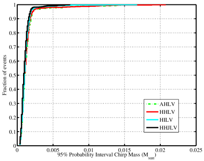
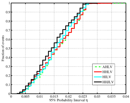
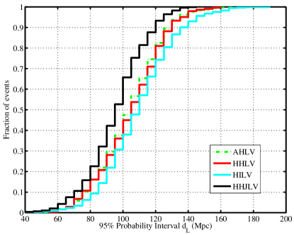
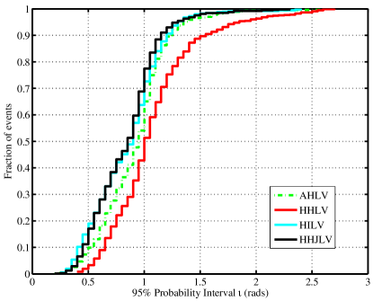
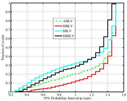
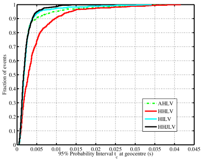
For a more detailed look at the performance of the networks for the non-sky-location parameters, we show in figure 5 the cumulative probability distributions for the fraction of signals found within a given probability interval width for , , , , and . Although our range of injections at constant distance is astrophysically unrealistic, these figures give a good idea of the relative performance of the networks across an isotropic distribution of sky position, polarisation and inclination angles. We can see immediately that the improvement in the resolution of the chirp mass and parameters is marginal, as evident from tables 4. The slightly improved performance for HHJLV can be attributed to the higher signal-to-noise ratio in that network thanks to the fifth detector.
With the distance and inclination angle parameters, we see slight improvements, with the biggest effect again being produced by the additional SNR in the HHJLV network. Due to degeneracies in the parameter space, the effect is more pronounced when the two dimensional distribution is considered, as in section IV.3. From table 4, we see that the median relative improvement of the polarization angle resolution is minimal, however in figure 5 it is apparent that for the 4-site networks there are a greater fraction of injections which are resolved well. This is explained by the large fraction of signals () which have a very broad distribution where the parameter is degenerate with the phase of the signal, when is close to 0 or . Although the median of the improvement ratio for individual sources is , the mean is for HALV and for HILV and HHJLV, indicating that the sources which can be resolved in are better resolved in the 4-site networks. The distribution shows similar performance for all 4-site networks for most signals, with slightly fewer signals poorly resolved in time with the HILV network than AHLV, reflecting the shorter tails of the distributions in figures 1 and 2 (sky localization is strongly correlated with the accuracy of timing the gravitational wave at the geocenter).
| Network | Median 95% conf. int. |
|---|---|
| AHLV | 6.625 deg2 |
| HHLV | 30.25 deg2 |
| HILV | 9 deg2 |
| HHJLV | 9.5 deg2 |
Fisher matrix results
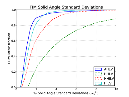
The Fisher information matrix results are presented in table 4. These are ratios of the median standard deviations for each parameter, taken from a Monte Carlo over angles (with distance adjusted to keep the total network SNR equal to 30). According to the FIM results, the greatest change in sky localization comes from the improvement in the measurement of the declination angle with a network that includes an Australian detector. The declination angle can be measured more accurately by a factor of with an AHLV network relative to the HHLV network, as a detector in the Southern hemisphere greatly improves the latitudinal baseline of the network, allowing for superior angular resolution in that direction. The last line in table 4 indicates the Fisher-matrix estimate of the sky area, defined following Eq. (43) of Barack and Cutler (2004). Figure 2 shows a histogram of the sky-area accuracy for two network configurations.
IV.3 Parameter Degeneracies
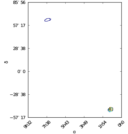
In cases where a signal is observed with marginal SNR in one or more detectors, or when the orientation of the binary is unfavourable (i.e. is close to ), a degeneracy between two sky locations often emerges. The addition of the fourth site to the network ensures that the source can be localised to a single region on the sky, as shown in the 2-dimensional PDFs of figure 4 which compares the 95% probability regions for different networks but the same injection. Note the two areas on the sky in the left panel, indicating a degeneracy that exists in a network with three sites but is removed when a fourth site is added.
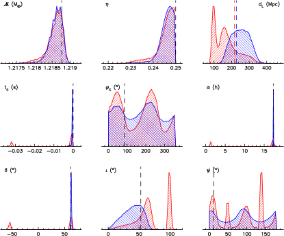
Moderate improvements also appear in inclination and luminosity distance measurements. Here, the one-dimensional estimators used in Tables 4, 4 and 4 do not tell the full story because of the strong correlation between inclination and luminosity distance. The secondary maximum on the sky position also corresponds to a secondary mode in the parameter corresponding to the transformation . In fact, the addition of a fourth site allows this degeneracy to be broken, as can be seen by comparing the marginalized one-dimensional PDFs for a sample injection the HHLV and AHLV network configurations, plotted in figure 3. Although the width did not shrink significantly from red to blue posteriors, with the AHLV network configuration the posteriors are unimodal and centered on the true values, as a degeneracy in the inclination-distance space is broken.
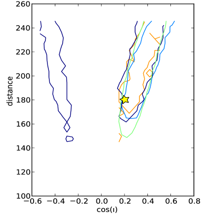
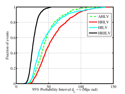
Both these effects are clearly visible in figure 4, which shows the breaking of the degeneracy in space as projected onto the and planes. In this example all the expanded networks allow the secondary maximum to be eliminated. Figure 6 shows the cumulative distribution of the 95% probability region for the space, with the improvement in two dimensions more prominent than looking at or individually (c.f. figure 5).
On the other hand, the accuracy with which mass parameters are measured does not improve as a consequence of moving the site of the fourth detector to India or Australia. We can speculate that the reason for this is that information about masses comes primarily from the phase evolution of the signal, and the accuracy in mass estimation is predominantly set by the overall network SNR. Meanwhile, masses do not strongly correlate with extrinsic parameters (with the exception of the time of coalescence), so their estimation is not significantly improved by better sky localization or inclination measurements.
The results from the Fisher information matrix are in qualitative agreement with the two Bayesian approaches regarding the partial breaking of the distance/inclination degeneracy achieved by moving a detector to Australia or India (leading to marginal improvements in both parameters, see table 4). They also indicate that the accuracy with which masses can be measured is not affected by the network choice.
V Conclusions
In this paper we studied the effect on parameter estimation of different networks of advanced detectors. We employed two different Bayesian techniques and the Fisher information matrix to estimate the accuracy of parameter recovery. We analysed a set of injections distributed in a grid in the extrinsic parameter space (without varying the mass and distance of injections) with the Inspnest code, and verified the results with LALInferenceMCMC . We performed a large scale Monte Carlo simulation using the Fisher matrix method with constant-SNR injections. We found consistent results between the three methods, pointing to significant gains in sky localization (typically by a factor of —) and modest gains in distance and inclination measurements with a network including a fourth site. We found that the 4-site networks are able to better resolve the polarisation angle of the source, in the cases where this is possible. We found no significant effect on mass measurements.
Comparing the different network configurations, we found, as expected, the strongest improvement in sky localization capability when the longest baseline (namely AHLV) was used, but that a site in India also provides a significant improvement in sky resolution. The HHJLV network, with the shortest extra baseline, provides the weakest improvement in sky resolution at a fixed signal-to-noise ratio; however, the fifth detector in this network can mitigate this, for an overall performance similar to HILV, but with fewer signals in the tail of the distribution with poor resolution.
We also find good agreement with previous work. In particular, Fairhurst Fairhurst (2011) finds 20-50% of signals localised within 20 for HHLV, and up to 20% within 5 with HHJLV, for an ensemble of sources at fixed distance of Mpc, in good agreement with figure 1. Despite the use of a different population of sources, Nissanke et al Nissanke et al. (2011) find results which qualitatively agree with our own. Comparison of the Fisher matrix results in figure 2 with Wen and Chen Wen and Chen (2010) shows good qualitative agreement with their expected distribution for the HLV network at fixed SNR of 15, when taking into account a factor of for the difference in SNR used (30 in our case, 15 in theirs).
In the present study, we focused on binary neutron stars (NS), which are the most “confident” source for the advanced detectors, but which are not expected to have significant spins Mandel and O’Shaughnessy (2010). On the other hand, black holes (BH) in NS-BH or BH-BH binaries can be rapidly spinning. Previous studies (see, e.g., van der Sluys et al. (2008b)) have shown that the presence of spin in one or both binary components can aid sky localization by providing additional polarization information through the precession inherent in misaligned spinning binaries. Localization may be further enhanced when a signal from a spinning binary is captured by a four-detector network; on the other hand, improved resolution of extrinsic parameters with the help of a fourth detector site may aid in the reconstruction of astrophysically interesting quantities such as spin-orbit misalignment angles.
The improved ability to localize sources on the sky will be crucial in any search for electromagnetic counterparts to detected gravitational-wave signals (e.g., Bloom et al. (2009); Nuttall and Sutton (2010); Mandel et al. (2011)). Accurate measurements of the location of the merging binary can also be useful even in the absence of electromagnetic counterparts, for example, in measuring typical binary kick velocities Kelley et al. (2010). We thus conclude that scientific considerations strongly favor an international gravitational wave network with four or more sites.
Acknowledgements
The authors would like to thank B. S. Sathyprakash, Stephen Fairhurst, Samaya Nissanke, and Jonathan Gair for useful discussions, and Kazuaki Kuroda for providing the LCGT noise curve. JV and BA were supported by the Science and Technology Facilities Council. IM was partially supported by the NSF Astronomy and Astrophysics Postdoctoral Fellowship, award AST-0901985; IM is also grateful for the hospitality of the Aspen Center for Physics during the end stages of preparing this paper. BF acknowledges the NSF GK-12 grant, award DGE-0948017. VR and VK acknowledge NSF grant PHY-0969820. CR acknowledges a Northwestern University graduate fellowship. AV was partially supported by the Science and Technology Facilities Council of the United Kingdom
*
Appendix A False alarm probabilities in a coherent search
It is instructive to ask how different network configurations affect false alarm probabilities (FAPs), or, alternatively, what the detection thresholds would need to be for a fixed FAP. We consider only the case of a fully coherent search; the FAP of triggers in searches that only require coincidence between detectors in mass and time of coalescence parameters, such as Abadie et al. (2010b, 2011), should not depend on the accuracy of measuring the sky location and other extrinsic parameters. If a coherent search is used, and all detectors are assumed to have independent noise, we might expect that the coherence constraint would be stronger for two co-located detectors that should have the same signal, and therefore HHLV should have a lower FAP than AHLV or HILV for a fixed network SNR.
We provide a Bayesian treatment of this question by comparing the odds ratio between the coherent signal hypothesis and the noise hypothesis for different network configurations. The odds ratio is just the ratio of posterior probabilities for the two models,
| (4) |
The only term that depends on the network configuration is the evidence for the presence of a signal, , which can be written as
| (5) |
We assume for the sake of simplicity that the prior is constant in the small region where the likelihood is significant, and the likelihood is Gaussian in the model parameters about a maximum at (as assumed for the Fisher matrix calculation),
| (6) |
This yields
| (7) |
where is the covariance matrix of the parameters, is the dimensionality of the model, and is the maximum likelihood of the data, given by
| (8) |
For a fixed network SNR (maximum likelihood), the evidence is therefore proportional only to , which scales with the size of the region in parameter space to which a signal’s parameters can be constrained.
Thus, for a fixed SNR, the Bayes factor is larger when parameters are less precisely estimated. Due to the shrinking size of the posterior distribution in sky location, distance and inclination, we might expect a decrease by a factor of in the allowed fraction of the prior volume between the HHLV and AHLV or HILV networks. Then, for a fixed detection threshold , the odds ratio will be a factor smaller for the AHLV or HILV network than for the HHLV network. Conversely, if we want to keep the same false alarm probability (same minimal odds ratio required for detection), the SNR threshold for the AHLV or HILV network must increase by relative to the HHLV network. This corresponds to a very modest increase in the SNR: for example, if the threshold is for the HHLV network, it will only rise to for the AHLV or HILV network.
The analysis above assumes that the noise in all interferometers is uncorrelated. While that is a reasonable assumption for distant interferometers, various environmental factors can lead to correlated noise in co-located interferometers, such as the two possible detectors at Hanford. This correlation can increase the threshold necessary for detection. For example, at times when only two of the four detectors in our presumed network are operational, it may not be possible to make a convincing detection if only the two Hanford detectors are operating from the HHLV network, while any two detectors from the AHLV or HILV network have a chance to detect a sufficiently loud signal.
References
- Bloom et al. (2009) J. S. Bloom et al. (2009), eprint 0902.1527.
- Nuttall and Sutton (2010) L. K. Nuttall and P. J. Sutton, Phys. Rev. D 82, 102002 (2010).
- Abbott et al. (2009) B. P. Abbott et al. (The LIGO Scientific Collaboration), Reports on Progress in Physics 72, 076901 (2009), URL http://stacks.iop.org/0034-4885/72/i=7/a=076901.
- Acernese et al. (2008) F. Acernese et al. (The Virgo Collaboration), Classical and Quantum Gravity 25, 184001 (2008), URL http://stacks.iop.org/0264-9381/25/i=18/a=184001.
- Grote and the LIGO Scientific Collaboration (2008) H. Grote and the LIGO Scientific Collaboration, Classical and Quantum Gravity 25, 114043 (2008).
- Harry and the LIGO Scientific Collaboration (2010) G. M. Harry and the LIGO Scientific Collaboration, Classical and Quantum Gravity 27, 084006 (2010).
- AdV (2009) Virgo Technical Report VIR-0027A-09, Virgo (2009).
- Finn et al. (2010) S. Finn, P. Fritschel, S. Klimenko, F. Raab, B. Sathyaprakash, P. Saulson, and R. Weiss, LIGO Document LIGO-T1000251, The LIGO Scientific Collaboration (2010), https://dcc.ligo.org/cgi-bin/DocDB/ShowDocument?docid=11604.
- Kuroda (2010) K. Kuroda (The LCGT Collaboration), Class. Quantum Grav. 27, 4004 (2010).
- Abadie et al. (2010a) J. Abadie et al. (The LIGO Scientific Collaboration), Classical and Quantum Gravity 27, 3001 (2010a).
- Jaranowski et al. (1996) P. Jaranowski, K. D. Kokkotas, A. Królak, and G. Tsegas, Classical and Quantum Gravity 13, 1279 (1996).
- Fairhurst (2009) S. Fairhurst, New Journal of Physics 11, 123006 (2009).
- Fairhurst (2011) S. Fairhurst, Classical and Quantum Gravity 28, 105021 (2011).
- Schutz (2011) B. F. Schutz (2011), eprint 1102.5421.
- Wen and Chen (2010) L. Wen and Y. Chen, Phys. Rev. D 81 (2010), eprint 1003.2504.
- Nissanke et al. (2011) S. M. Nissanke, J. L. Sievers, N. Dalal, and D. E. Holz (2011), eprint 1105.3184.
- Klimenko et al. (2011) S. Klimenko, G. Vedovato, M. Drago, G. Mazzolo, G. Mitselmakher, C. Pankow, G. Prodi, V. Re, F. Salemi, and I. Yakushin, Phys. Rev. D 83, 102001 (2011), eprint 1101.5408.
- van der Sluys et al. (2008a) M. van der Sluys, V. Raymond, I. Mandel, C. Röver, N. Christensen, V. Kalogera, R. Meyer, and A. Vecchio, Classical and Quantum Gravity 25, 184011 (2008a), eprint 0805.1689.
- van der Sluys et al. (2008b) M. V. van der Sluys, C. Röver, A. Stroeer, V. Raymond, I. Mandel, N. Christensen, V. Kalogera, R. Meyer, and A. Vecchio, Astrophysical Journal 688, L61 (2008b), eprint 0710.1897.
- Raymond et al. (2009) V. Raymond, M. V. van der Sluys, I. Mandel, V. Kalogera, C. Röver, and N. Christensen, Classical and Quantum Gravity 26, 114007 (2009), eprint 0812.4302.
- Gilks et al. (1996) W. R. Gilks, S. Richardson, and D. J. Spiegelhalter, Markov chain Monte Carlo in practice (Chapman & Hall/CRC, 1996).
- Veitch and Vecchio (2008) J. Veitch and A. Vecchio, Classical and Quantum Gravity 25, 184010 (2008).
- Veitch and Vecchio (2010) J. Veitch and A. Vecchio, Phys. Rev. D 81, 062003 (2010).
- Skilling (2006) J. Skilling, Bayesian Analysis 1, 833 (2006).
- Röver et al. (2006) C. Röver, R. Meyer, and N. Christensen, Classical and Quantum Gravity 23, 4895 (2006), eprint arXiv:gr-qc/0602067.
- (26) LSC Algorithm Library software, http://www.lsc-group.phys.uwm.edu/lal.
- Kuroda (2011) K. Kuroda (2011), Private communication.
- Cutler and Flanagan (1994) C. Cutler and E. Flanagan, Phys. Rev. D 49, 2658 (1994).
- Vallisneri (2008) M. Vallisneri, Phys. Rev. D 77 (2008).
- Blanchet et al. (1996) L. Blanchet, B. R. Iyer, C. M. Will, and A. G. Wiseman, Class. Quantum Grav. 13, 575 (1996).
- Buonanno et al. (2009) A. Buonanno, B. R. Iyer, E. Ochsner, Y. Pan, and B. S. Sathyaprakash, Phys. Rev. D 80, 084043 (2009), eprint 0907.0700.
- Damour et al. (2001) T. Damour, B. R. Iyer, and B. S. Sathyaprakash, Phys. Rev. D 63, 044023 (2001).
- Jeffreys (1946) H. Jeffreys, Proc. R. Soc. Lond. A 186, 453 (1946).
- Barack and Cutler (2004) L. Barack and C. Cutler, Phys. Rev. D 69, 082005 (2004).
- Mandel and O’Shaughnessy (2010) I. Mandel and R. O’Shaughnessy, Classical and Quantum Gravity 27, 114007 (2010), eprint 0912.1074.
- Mandel et al. (2011) I. Mandel, L. Z. Kelley, and E. Ramirez-Ruiz, ArXiv e-prints (2011), eprint 1111.0005.
- Kelley et al. (2010) L. Z. Kelley, E. Ramirez-Ruiz, M. Zemp, J. Diemand, and I. Mandel, Astrophysical Journal 725, L91 (2010), eprint 1011.1256.
- Abadie et al. (2010b) J. Abadie et al. (LIGO Scientific Collaboration and Virgo Collaboration), Phys. Rev. D 82, 102001 (2010b), eprint 1005.4655.
- Abadie et al. (2011) J. Abadie et al. (LIGO Scientific Collaboration and Virgo Collaboration), Submitted to PRD (2011), eprint arXiv:1102.3781.
- Nissanke et al. (2010) S. Nissanke, D. E. Holz, S. A. Hughes, N. Dalal, and J. L. Sievers, Astrophysical Journal 725, 496 (2010), eprint 0904.1017.