Can Self–Organizing Maps accurately predict photometric redshifts?

Abstract

We present an unsupervised machine learning approach that can be employed for estimating photometric redshifts. The proposed method is based on a vector quantization approach called Self–Organizing Mapping (SOM). A variety of photometrically derived input values were utilized from the Sloan Digital Sky Survey’s Main Galaxy Sample, Luminous Red Galaxy, and Quasar samples along with the PHAT0 data set from the PHoto-z Accuracy Testing project. Regression results obtained with this new approach were evaluated in terms of root mean square error (RMSE) to estimate the accuracy of the photometric redshift estimates. The results demonstrate competitive RMSE and outlier percentages when compared with several other popular approaches such as Artificial Neural Networks and Gaussian Process Regression. SOM RMSE–results (using $\Delta$z=z_phot–z_spec) for the Main Galaxy Sample are 0.023, for the Luminous Red Galaxy sample 0.027, Quasars are 0.418, and PHAT0 synthetic data are 0.022. The results demonstrate that there are non–unique solutions for estimating SOM RMSEs. Further research is needed in order to find more robust estimation techniques using SOMs, but the results herein are a positive indication of their capabilities when compared with other well-known methods.

1. Introduction

There is a pressing need for accurate estimates of galaxy photometric redshifts (photo–z’s) as demonstrated by the increasing number of papers on this topic and especially by recent attempts to objectively compare methods (e.g. Hildebrandt et al., 2010; Abdalla et al., 2011). The need for photo-z’s will only increase as larger and deeper surveys such as Pan-STARRS(Kaiser, 2004), LSST(Ivezic et al., 2008) and Euclid (Sorba & Sawicki, 2011) come on–line in the coming decade. The photometric–only surveys (Pan-STARRS, LSST) will have relatively small numbers of follow-up spectroscopic redshifts and will rely upon either template-fitting methods such as Bayesian Photo-z’s (Benítez, 2000) Le Phare (Ilbert et al., 2006), or training-set methods such as those discussed herein. The Euclid mission may include a slitless spectrograph offering far more training–set galaxies.

A diverse set of regression techniques using training–set methods have been applied to the problem of estimating photometric redshifts in the past 10 years. These include Artificial Neural Networks (Firth et al., 2003; Tagliaferri et al., 2003; Ball et al., 2004; Collister & Lahav, 2004; Vanzella et al., 2004), Decision Trees (Suchkov et al., 2005), Gaussian Process Regression (Way & Srivastava, 2006; Foster et al., 2009; Way et al., 2009; Bonfield et al., 2010; Way, 2011), Support Vector Machines (Wadadekar, 2005), Ensemble Modeling (Way et al., 2009), Random Forests Carliles et al. (2008), and Kd–Trees (Csabai et al., 2003) to name but a few.

On the other hand, even though Self–Organizing Maps (SOMs) have been used extensively in a number of other scientific fields (the paper that opened the field, Kohonen (1982), currently has over 2000 citations) they have been used sparingly thus far in Astronomy (e.g. Mahdi, 2011; Naim et al., 1997; Way, Gazis & Scargle, 2011), and only this year in estimating photometric redshifts (Geach, 2011).

In this work we attempt to use SOMs to estimate photometric redshifts for several Sloan Digital Sky Survey (SDSS, York et al., 2000) derived catalogs of different galaxy types, including Quasars along with the PHAT0 data set of Hildebrandt et al. (2010). In Section 2 we describe the input data sets used, in Section 3 we give an overview of SOMs, and some conclusions in Section 4.

2. Data

Three different data sets derived from the SDSS Data Release Seven (DR7, Abazajian et al., 2009) were used. They include the Main Galaxy Sample (MGS, Strauss et al., 2002) the Luminous Red Galaxy Sample (LRG, Eisenstein et al., 2001), and the Quasar sample (QSO, Schneider et al., 2007). Data from the Galaxy Zoo (Lintott et al., 2008) Data Release 1 (Lintott et al., 2011) survey results were used to segregate galaxies as Spiral or Elliptical in the case of the MGS and LRG samples. Details of how this was done are given in Way (2011). Dereddened magnitudes (u,g,r,i,z) were used as inputs in all scenarios. The same SDSS photometric and redshift quality flags on the input variables were used as in Way (2011). In addition we used the simulation–based PHAT0 data set (see Hildebrandt et al., 2010) which was constructed to to test a variety of different photo–z estimation methods. The PHAT0 data set consists of 5 SDSS like filters (u,g,r,i,z) used on MEGACAM at CFHT (Boulade et al., 2003) with an additional 6 input filters (Y,J,H,K,Spitzer IRAC [3.6], Spitzer IRAC [4.5]) giving a total of 11 filters spanning a range of 4000Å to 50,000Å. This large range should help to avoid color–redshift degeneracies that can occur if ultraviolet or infrared bandpasses are not used (Benítez, 2000). The PHAT0 synthetic photometry was created from the Le Phare photo-z code (Arnouts et al., 2002; Ilbert et al., 2006). Initially Le Phare creates noise free data, but given the desire to test more real–world conditions we utilized the PHAT0 data with added noise. A parametric form was used for the signal–to–noise as a function of magnitude where it acts as an exponential at fainter magnitudes and a power–law a brighter ones. The magnitude cut between these two regimes is filter dependent and is given in Table 2 of Hildebrandt et al. (2010). The larger of two catalogs was used herein (as suggested for training–set methods) that contains $\sim$ 170,000 objects.

Since we use a training–set method our original data sets are split into training=89%, testing=10% and validation=1%. Validation was only used in the Artificial Neural Network algorithm discussed in the next section. The full size of each input data set are listed in parentheses in column 1 of Table 1.

3. Methods

Several methods in use for calculating photometric redshifts were compared with the SOM results: the Artificial Neural Network code of Collister & Lahav (2004) (ANNz), the Gaussian Process Regression code of Foster et al. (2009) (GPR), as well as simple Linear and Quadratic regression. The latter is comparable to that of the Polynomial fits used by Li & Yee (2008). Both the ANNz and GPR codes are freely downloadable. Details on the ANNz and GPR algorithms can be found in their respective citations above.

Table 1Results

Data	Method		$\sigma_{RMSE}$		Outlier
		50%	10%	90%
MGS	GPR	0.02087	0.02072	0.02096	0.11629
(455803)	ANNz	0.02044	–	–	0.14482
–	SOM	0.02339	–	–	0.1689
–	Linear	0.02742	0.02729	0.02758	0.35986
–	Quadratic	0.02494	0.02412	0.02762	0.29184
LRG	GPR	0.02278	0.02256	0.02309	0.41898
(143221)	ANNz	0.02138	–	–	0.41176
–	SOM	0.02689	–	–	0.64292
–	Linear	0.02896	0.02896	0.02897	0.71516
–	Quadratic	0.02382	0.02376	0.02402	0.45510
MGS–ELL	GPR	0.01455	0.01434	0.01473	0.06591
(45521)	ANNz	0.01442	–	–	0.06591
–	SOM	0.02044	–	–	0.10984
–	Linear	0.01745	0.01731	0.01756	0.19772
–	Quadratic	0.01612	0.01609	0.01629	0.10984
MGS–SP	GPR	0.02078	0.02061	0.02093	0.13305
(120266)	ANNz	0.01991	–	–	0.05821
–	SOM	0.02426	–	–	0.04158
–	Linear	0.02539	0.02529	0.02555	0.28272
–	Quadratic	0.02326	0.02296	0.02607	0.20788
LRG–SP	GPR	0.01416	0.01397	0.01436	0.00000
(13708)	ANNz	0.01516	–	–	0.00000
–	SOM	0.01848	–	–	0.07299
–	Linear	0.01635	0.01627	0.01649	0.07299
–	Quadratic	0.01469	0.01462	0.01477	0.00000
LRG–ELL	GPR	0.01186	0.01162	0.01224	0.00000
(27378)	ANNz	0.01298	–	–	0.10961
–	SOM	0.01568	–	–	0.00000
–	Linear	0.01362	0.01361	0.01364	0.10961
–	Quadratic	0.01263	0.01254	0.01274	0.07307
QSO	GPR	0.37342	0.03967	0.37626	50.96627
(56923)	ANNz	0.65802	–	–	88.54533
–	SOM	0.41821	–	–	54.23401
–	Linear	0.57061	0.57010	0.57102	84.64512
–	Quadratic	0.53972	0.53679	0.54539	81.27196
phat0	GPR	0.01487	0.01436	0.01532	0.03539
(169520)	ANN	0.01805	–	–	0.05309
–	SOM	0.02236	–	–	0.37754
–	Linear	0.08703	0.08702	0.08704	19.34875
–	Quadratic	0.02436	0.02433	0.02438	0.19467

The main purpose of Self–Organized mapping is the ability of SOMs to transform a feature vector of arbitrary dimension drawn from the given feature space of photometric inputs (e.g., the SDSS u,g,r,i,z magnitudes) into simplified 1– or 2–dimensional discrete maps. The method was originally developed by Kohonen (1982, 2001) to organize information in a logical manner. This type of machine learning utilizes an unsupervised learning scheme of vector quantization, known as competitive learning in the field of neural information processing. It is useful for analyzing complex data with a–priori unknown relationships that are visualized by the self-organization process (Kohonen, 2001).

A SOM is structured in two layers: an input layer and a Kohonen layer (Figure 1). For example, the Kohonen layer could represent a structure with a single 2–dimensional map (lattice) consisting of neurons arranged in rows and columns. Each neuron of this discrete lattice is fixed and is fully connected with all source neurons in the input layer. For the given task of estimating photometric redshifts, a 5–dimensional feature vector of the u,g,r,i,z magnitudes is defined. One feature vector (u,g,r,i,z) is presented to 5 input layer neurons. This typically activates (stimulates) one neuron in the Kohonen layer. Learning occurs during the self–organizing procedure as feature vectors drawn from a training data set are presented to the input layer of the SOM network (Figure 1a). These feature vectors are also referred to as input vectors. Neurons of the Kohonen layer compete to see which neuron will be activated by the weight vectors that connect the input neurons and Kohonen neurons. In other words, the weight vectors identify which input vector can represented by a single Kohonen neuron. Hence, they are used to determine only one activated neuron in the Kohonen layer after the winner–takes–all principle (Figure 1b).

The SOM is considered as trained after learning, at which time the weights of the neurons have stored the inter–relations of all 5–dimensional u,g,r,i,z feature vectors. Then, known spectroscopic redshift values for all input vectors of a test data set that are represented by a single Kohonen neuron are averaged (Fig.1b). The redshift mean value represents all 5–D u,g,r,i,z vectors that are similar to the weight vector of the activated Kohonen neuron. The more Kohonen neurons there are the more precisely each input vector can be represented by a weight vector. However, the total number of Kohenen neurons are optimized for each data set (see Figure 2). A practical overview about the learning/training process is described by Klose (2006); Klose et al. (2008, 2010) and in much greater detail by Kohonen (2001).

After training, the u,g,r,i,z input vectors of a test data set are presented to a trained SOM. At the end of a classification step, every Kohonen neuron approximates an input vector whereby similar/dissimilar input data were represented by neighboring/distant neurons. One neuron could even classify several input vectors, if these input vectors were very similar compared to the other given input vectors. Results from the photometric redshift approximations are then compared to known spectroscopic redshift data. Regression performance is estimated based on the root mean square error (RMSE) of the predicted photometric redshifts and the known spectroscopic redshifts (using $\Delta$z=z_phot–z_spec). To reiterate, during the training phase, each Kohonen neuron identifies a certain number of galaxies that are characterized by similar u,g,r,i,z intensities. Photometric redshift data were then averaged for these intensity values.

The SOM approximates the input feature space and maps it into an output space. The output space shows the SOM approximation as a 2-D map (Haykin, 2009). Best results can be obtained with an optimization scheme such that the RMSE of the test data set is minimal as illustrated in Figure 2. Accuracy (e.g. RMSE) depends on the size of the Kohonen map. The number of neurons in the Kohonen map can be considered a regularization parameter ($\xi$) as shown in Figure 2.

Figure 2 shows that RMSE is high when the number of Kohonen neurons is too small ($\xi<$2000) or too large ($\xi>$10000) and hence that the 5–dimensional u,g,r,i,z–input space is underfit or overfit. Theoretically, a global minimum of the RMSE–curve might exist. However, the input feature space for the given photometric redshift problem shows a very rough RMSE–curve (Figure 2) with at least 2 local minima. In this case it is clear that SDSS redshift estimation tends to have several local minima, which makes is important to chose the right optimization method to determine the SOM network size. On the other hand, the smoother the RMSE–curve is the better gradient methods can be utilized. Evolution strategies or genetic programming could be applied to rougher curves with many local minima. This in turn can make it cumbersome to find fast back–propagation Artificial Neural Network (ANN) structures, especially when data sets are small.

Another advantage of SOMs in comparison to ANNs is that there is no need to optimize the structure of SOMs (e.g., number of hidden layers), since it is based on unsupervised learning.

Only the size of the Kohonen map needs to be optimized for each data set. SOMs also allow non–experts to visualize the redshift estimates in relation to the multi–dimensional input space. This eliminates the often criticized “black box” problem of ANNs. As mentioned previously, SOMs approximate the input feature space while ANNs typically separate them into sub–regions. Finally, SOMs are known to be powerful when very small data sets are available for training (see, Haykin, 2009).

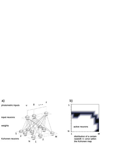
Figure 1.— Schematic illustration of the structure (a) and functionality (b) of a Self–Organizing Map with $I$ input neurons and $M\times N$ Kohonen neurons. The SOM visualizes the structure of the $I$–dimensional input space. In this case, the SOM illuminates a certain redshift$\pm$error within the Kohonen map and as a function of the input space.

Figure 2.— Accuracy (RMSE) versus regularization parameter value $\xi$ for the LRG–ELL data set (see Table 1). Different classifications will result from different choices of the $\xi$ value. The regularization value is defined by the number of Kohonen neurons, which is maximum with respect to the training data set. The convex curve has a two local minima at $\xi$=4100 and $\xi$=5100. The roughness of this RMSE cost function shows that traditional gradient based optimization strategies, e.g. deterministic annealing, might result in sub–optimal solutions. Other methods, such as, genetic programming might find the global minimum much faster.

Figure 3.— Results from the three methods using SDSS u–g–r–i–z dereddened magnitudes as inputs for the SDSS DR7 Luminous Red Galaxies classified as ellipticals by the GalaxyZoo team. The bottom two plots show the SOM results for the two local minima described in Section 3 and shown in Figure 2

4. Conclusion

SOMs offer a competitive choice in terms of low RMSE, algorithm comprehension (also see Göppert & Rosenstiel (1993)) and percentage of outliers. The final results are presented in Table 1 and plots for the LRG–ELL data set for the SOM, ANNz and GPR methods are shown in Figure 3

As mentioned previously, obtaining the global minimum is important and, not surprisingly, can affect the results. Figure 2 shows the two local minima ($\xi$=4100 and 5100) listed for the LRG–ELL (Luminous Red Galaxies classified as Ellipticals by GalaxyZoo) data set in Table 1. Clearly there are a number of other $\xi$–values and the RMSE will be greatly affected by the choice as seen on the y–axis of Figure 2 for a given $\xi$–value. Given these facts, the roughness of the RMSE cost function in Figure 2 shows that traditional gradient based optimization strategies, e.g, deterministic annealing, might yield sub–optimal solutions. Other methods, such as, genetic programming might find the “global” minimum much faster, if a global minima exists with respect to the uncertainties of the RMSE.

During completion of this manuscript another paper using SOMs for classification and photometric estimation was released (Geach, 2011). Our work differs in that we mostly focus on a wider variety of low–redshift samples drawn from the SDSS, while (Geach, 2011) focuses more on the higher redshift samples akin to those used in Hildebrandt et al. (2010).

We have shown that SOMs are a powerful tool for estimating photometric redshifts and that with additional work they are sure to be useful in future surveys with limited numbers of follow–up spectroscopic redshifts.

References

- Abazajian et al. (2009) Abazajian, K.N. et al. 2009, ApJS, 182, 543
- Abdalla et al. (2011) Abdalla, F.B., Banerji, M., Lahav, O. & Rashkov, V. 2011, MNRAS, 417, 1891
- Arnouts et al. (2002) Arnouts, S., Moscardini, L., Vanzella, E., et al. 2002, MNRAS, 329, 355
- Ball et al. (2004) Ball, N.M., Loveday, J., Fukugita, M., Nakamura, O., Okamura, S., Brinkmann, J., & Brunner, R.J. 2004, MNRAS, 348, 1038
- Benítez (2000) Benítez, N. 2000, ApJ, 536, 571
- Bonfield et al. (2010) Bonfield, D.G., Sun, Y., Davey, N., Jarvis, M.J., Abdalla, F.B., Banerji, M., & Adams, R. G. 2010, MNRAS, 405, 987
- Boulade et al. (2003) Boulade, O., Charlot, X., Abbon, P., et al. 2003, ed. M. Iye, & A. F. M. Moorwood, SPIE Conf. Ser., 4841, 72
- Carliles et al. (2008) Carliles, S., et al. 2008, ASPC, 394, 521
- Collister & Lahav (2004) Collister, A. A. & Lahav, O. 2004, PASP, 116, 345
- Csabai et al. (2003) Csabai, I., et al. 2003, AJ, 125, 580
- Eisenstein et al. (2001) Eisenstein et al. 2001, AJ, 122, 2267
- Firth et al. (2003) Firth, A.E., Lahav, O., & Somerville, R.S. 2003, MNRAS, 339, 1195
- Foster et al. (2009) Foster, L., Waagen, A., Aijaz, N. et al. 2009, Journal of Machine Learning Research, 10, 857
- Gazis, Levit, & Way (2010) Gazis, P.R., Levit, C. & Way, M.J. 2010, PASP, 122, 1518
- Geach (2011) Geach, J.E. 2011, arXiv:1110.0005, MNRASin Press
- Göppert & Rosenstiel (1993) Göppert, J. & Rosenstiel, W. 1993, “Self-organizing Maps vs. Backpropagation: An Experimental Study”, Proc. of Workshop on Design Methodologies for Microelectronis and Signal Processing, pp. 153–162, Giwice, Poland.
- Haykin (2009) Haykin, S.S. 2009, “Neural networks and learning machines”, v.10, Prentice Hall, ISBN 9780131471399
- Hildebrandt et al. (2010) Hildebrandt et al. 2010, A&A, 523, A31
- Ilbert et al. (2006) Ilbert, O., Arnouts, S., McCracken, H. J., et al. 2006, A&A, 457, 841
- Ivezic et al. (2008) Ivezic, Z., Tyson, J.A., Allsman, R., Andrew, J., Angel, R., et al 2008, arXiv:0805.2366v1
- Kaiser (2004) Kaiser, N. 2004, “Pan-STARRS: a wide-field optical survey telescope array”, SPIE, 5489, 11-12
- Klose (2006) Klose, C.D. 2006, Computational Geosciences; 10(3), 265-277
- Klose et al. (2008) Klose, C.D., A.D., Netz, U., Scheel, A.K., Beuthan, J., Hielscher, A.H. Biomed Opt 13(5):050503
- Klose et al. (2010) Klose, C.D., A.D., Netz, U., Scheel, A.K., Beuthan, J., Hielscher, A.H. 2010, Biomed Opt 15(6):066020
- Kohonen (1982) Kohonen, T. 1982 Biol. Cyb., 43(1): 59-69
- Kohonen (2001) Kohonen, T. 2001, Self–Organizing Maps, 3rd edition, Springer, Berlin.
- Li & Yee (2008) Li, I.H. & Yee, H.K.C. 2008, AJ, 135, 809
- Lintott et al. (2008) Lintott, C., Schawinski, K., Slosar, A. et al. 2011, MNRAS, 389, 1179
- Lintott et al. (2011) Lintott, C., Schawinski, K., Bamford, S. et al. 2011, MNRAS, 410, 166
- Mahdi (2011) Mahdi, B. 2011, arXiv:1108.0514
- Naim et al. (1997) Naim, A., Ratnatunga, K.U. & Griffiths, R.E. 1997, ApJS, 111, 357
- Schneider et al. (2007) Schneider, D.P., Hall, P.B., Richards, G.T. et al. 2007, AJ, 134, 102
- Sorba & Sawicki (2011) Sorba, R. & Sawicki, M. 2011, arXiv:1101.4635
- Strauss et al. (2002) Strauss, M.A., et al. 2002, AJ, 124, 1810
- Suchkov et al. (2005) Suchkov, A.A., Hanisch, R.J., & Margon, B. 2005, AJ, 130, 2439
- Tagliaferri et al. (2003) Tagliaferri, R., Longo, G., Andreon, S., Capozziello, S., Donalek, C., & Giordano, G. 2003, Lecture Notes in Computer Science, vol 2859, 226
- Vanzella et al. (2004) Vanzella, E., et al. 2004, A&A, 423, 761
- Wadadekar (2005) Wadadekar, Y. 2005, PASP, 117, 79
- Way, Gazis & Scargle (2011) Way, M.J., Gazis, P.R. & Scargle, J.D. 2011, ApJ, 727, 48
- Way & Srivastava (2006) Way, M.J. & Srivastava, A.N. 2006, ApJ, 647, 102
- Way et al. (2009) Way, M.J., Foster, L.V., Gazis, P.R. & Srivastava, A.N. 2009, ApJ, 706, 623
- Way (2011) Way, M.J. 2011, ApJ, 734, 9
- York et al. (2000) York, D.G., et al. 2000, AJ, 120, 1579