Sharp maximal inequalities for the moments of martingales and non-negative submartingales

Abstract

In the paper we study sharp maximal inequalities for martingales and non-negative submartingales: if $f$, $g$ are martingales satisfying

$$|\mathrm{d}g_{n}|\leq|\mathrm{d}f_{n}|,\qquad n=0,1,2,\ldots,$$

almost surely, then

$$\Bigl{\|}\sup_{n\geq 0}|g_{n}|\Bigr{\|}_{p}\leq p\|f\|_{p},\qquad p\geq 2,$$

and the inequality is sharp. Furthermore, if $\alpha\in[0,1]$, $f$ is a non-negative submartingale and $g$ satisfies

$$|\mathrm{d}g_{n}|\leq|\mathrm{d}f_{n}|\quad\mbox{and}\quad|\mathbb{E}(\mathrm{d}g_{n+1}|\mathcal{F}_{n})|\leq\alpha\mathbb{E}(\mathrm{d}f_{n+1}|\mathcal{F}_{n}),\qquad n=0,1,2,\ldots,$$

almost surely, then

$$\Bigl{\|}\sup_{n\geq 0}|g_{n}|\Bigr{\|}_{p}\leq(\alpha+1)p\|f\|_{p},\qquad p\geq 2,$$

and the inequality is sharp. As an application, we establish related estimates for stochastic integrals and Itô processes. The inequalities strengthen the earlier classical results of Burkholder and Choi.

1 Introduction

The purpose of the paper is to provide the best constants in some maximal inequalities for martingales and non-negative submartingales. Let us start with introducing the necessary notation. Let $(\Omega,\mathcal{F},\mathbb{P})$ be a non-atomic probability space, equipped with a filtration $(\mathcal{F}_{n})_{n\geq 0}$, that is, a non-decreasing family of sub-$\sigma$-fields of $\mathcal{F}$. Let $f=(f_{n})$ and $g=(g_{n})$ be adapted, real-valued integrable processes. The difference sequences $\mathrm{d}f=(\mathrm{d}f_{n})$ and $\mathrm{d}g=(\mathrm{d}g_{n})$ of $f$ and $g$ are defined by the equations

$$f_{n}=\sum_{k=0}^{n}\mathrm{d}f_{k},\qquad g_{n}=\sum_{k=0}^{n}\mathrm{d}g_{k},\qquad n=0,1,2,\ldots.$$

We are particularly interested in those pairs $(f,g)$ for which a certain domination relation is satisfied. Following Burkholder [6], we say that $g$ is differentially subordinate to $f$ if, for any $n\geq 0,$ we have

$$\mathbb{P}(|\mathrm{d}g_{n}|\leq|\mathrm{d}f_{n}|)=1.$$

As an example, let $g$ be a transform of $f$ by a predictable sequence $v=(v_{n})$ bounded in absolute value by $1$; that is, we have $\mathbb{P}(|v_{n}|\leq 1)=1$ and $\mathrm{d}f_{n}=v_{n}\,\mathrm{d}g_{n}$, $n\geq 0$. Here, by predictability, we mean that $v_{0}$ is $\mathcal{F}_{0}$-measurable and $v_{n}$ is $\mathcal{F}_{n-1}$-measurable for $n\geq 1$. In the particular case when each $v_{n}$ is deterministic and takes values in $\{-1,1\}$, we will say that $g$ is a $\pm 1$ transform of $f$.

Another domination we will consider is the so-called $\alpha$-strong subordination, where $\alpha$ is a fixed non-negative number. This notion was introduced by Burkholder in [10] in the special case $\alpha=1$ and extended to a general case by Choi [12]: The process $g$ is $\alpha$-strongly subordinate to $f$ if it is differentially subordinate to $f$ and, for any $n\geq 0$,

$$|\mathbb{E}(\mathrm{d}g_{n+1}|\mathcal{F}_{n})|\leq\alpha|\mathbb{E}(\mathrm{d}f_{n+1}|\mathcal{F}_{n})|$$

almost surely.

There is a vast literature concerning the comparison of the sizes of $f$ and $g$ under the assumption of one of the dominations above and the further condition that $f$ is a martingale or non-negative submartingale; we refer the interested reader to the papers [6, 9, 10, 12, 15, 16, 18, 19, 20, 21] and the references therein. In addition, these inequalities have found their applications in many areas of mathematics: Banach space theory [4, 5]; harmonic analysis [8, 13, 14]; functional analysis [6, 7, 20]; analysis [1, 2]; stochastic integration [6, 11, 17, 20, 21]; and more. To present our motivation, we state here only two theorems. Let us start with a fundamental result of Burkholder [6]. We use the notation $\|f\|_{p}=\sup_{n}\|f_{n}\|_{p}$, $p\in[1,\infty]$.

Theorem 1.1 ((Burkholder))

Assume that $f$, $g$ are martingales and $g$ is differentially subordinate to $f$. Then, for any $1<p<\infty$,

$$\|g\|_{p}\leq(p^{*}-1)\|f\|_{p},$$ (1)

where $p^{*}=\max\{p,p/(p-1)\}$. The constant $p^{*}-1$ is the best possible; it is already the best possible if $g$ is assumed to be a $\pm 1$ transform of $f$.

Here, by the optimality of the constant, we mean that for any $r<p^{*}-1$ there exists a martingale $f$ and its $\pm 1$ transform $g$, for which $\|g\|_{p}>r\|f\|_{p}$.

The submartingale version of the estimate above is the following result of Choi [12].

Theorem 1.2 ((Choi))

Assume that $f$ is a non-negative submartingale and $g$ is $\alpha$-differentially subordinate to $f$, $\alpha\in[0,1]$. Then for any $1<p<\infty$,

$$\|g\|_{p}\leq(p_{\alpha}^{*}-1)\|f\|_{p},$$ (2)

where $p_{\alpha}^{*}=\max\{(\alpha+1)p,p/(p-1)\}$. The constant is the best possible.

In the paper we deal with a considerably harder problem and determine the optimal constants in the related moment estimates involving the maximal functions of $f$ and $g$. For $n\geq 0$, let $f_{n}^{*}=\sup_{0\leq k\leq n}|f_{k}|$ and $f^{*}=\sup_{k\geq 0}|f_{k}|$. Here is our first main result.

Theorem 1.3

Let $f$, $g$ be martingales with $g$ being differentially subordinate to $f$. Then for any $p\geq 2$,

$$\|g^{*}\|_{p}\leq p\|f\|_{p}$$ (3)

and the constant $p$ is the best possible. It is already the best possible in the following weaker inequality: If $f$ is a martingale and $g$ is its $\pm 1$ transform, then

$$\|g^{*}\|_{p}\leq p\|f^{*}\|_{p}.$$ (4)

Note that the validity of the estimates (3) and (4) is an immediate consequence of (1) and Doob’s bound $\|f^{*}\|_{p}\leq\frac{p}{p-1}\|f\|_{p}$, $p>1$. The non-trivial (and quite surprising) part is the optimality of the constant $p$.

Now let us state the submartingale version of the theorem above.

Theorem 1.4

Fix $\alpha\in[0,1]$. Let $f$ be a non-negative submartingale and $g$ be real valued and $\alpha$-strongly subordinate to $f$. Then for any $p\geq 2$,

$$\|g^{*}\|_{p}\leq(\alpha+1)p\|f\|_{p}$$ (5)

and the constant $(\alpha+1)p$ is the best possible. It is already the best possible in the weaker estimate

$$\|g^{*}\|_{p}\leq(\alpha+1)p\|f^{*}\|_{p}.$$ (6)

There is a natural question: What is the best constant in the inequalities above in the case $1<p<2$? Unfortunately, we have been unable to answer it; our reasoning works only for the case $p\geq 2$.

The proof of (5) is based on a technique invented by Burkholder in [11]. It enables us to translate the problem of proving a maximal inequality for martingales to that of finding a certain special function, an upper solution to a corresponding nonlinear problem. The method can be easily extended to the submartingale setting (see [17]) and we construct the function in Section 3. For the sake of construction, we need a solution to a differential equation that is analyzed in Section 2. The next two sections are devoted to the proofs of the announced results: Section 4 contains the proof of the estimate (5) and the final part concerns the optimality of the constants appearing in (4) and (6). In the final section, we present some applications: sharp estimates for stochastic integrals and Itô processes.

2 A differential equation

For a fixed $\alpha\in(0,1]$ and $p\geq 2$, let $C=C_{p,\alpha}=[(\alpha+1)p]^{p}(p-1)$. A central role in the paper is played by a certain solution to the differential equation

$$\gamma^{\prime}(x)=\frac{-1+C(1-\gamma(x))\gamma(x)x^{p-2}}{1+C(1-\gamma(x))x^{p-1}}.$$ (7)

Lemma 2.1

There is a solution $\gamma\mathchoice{\nobreak\,\colon}{\nobreak\,\colon}{\nobreak\,\colon\;}{\nobreak\,\colon\;}[((\alpha+1)p)^{-1},\infty)\to\mathbb{R}$ of (7), satisfying the initial condition

$$\gamma\biggl{(}\frac{1}{(\alpha+1)p}\biggr{)}=1-[(\alpha+1)p]^{-1}.$$ (8)

The solution is non-decreasing, concave and bounded from above by $1$.

[Proof.] Let $\gamma$ be a solution to (7), satisfying (8) and extended to a maximal subinterval $I$ of $[((\alpha+1)p)^{-1},\infty)$. It is convenient to split the proof into a few steps.

Step 1: $I=[((\alpha+1)p)^{-1},\infty)$. In view of the Picard–Lindelöf theorem, this will be established if we show that $\gamma<1$ on $I$. To this end, suppose that the set $\{x\in I\mathchoice{\nobreak\,\colon}{\nobreak\,\colon}{\nobreak\,\colon\;}{\nobreak\,\colon\;}\gamma(x)=1\}$ is non-empty and let $y$ denote its smallest element. Then, by (7), we have $\gamma^{\prime}(y)=-1$, which, by minimality of $y$, implies $\gamma(((\alpha+1)p)^{-1})>1$ and contradicts (8).

Step 2: Concavity of $\gamma$. Suppose that the set $\{x\in I\mathchoice{\nobreak\,\colon}{\nobreak\,\colon}{\nobreak\,\colon\;}{\nobreak\,\colon\;}\gamma^{\prime\prime}(x)>0\}$ is non-empty and let $z$ denote its infimum. Consider the functions $F,G\mathchoice{\nobreak\,\colon}{\nobreak\,\colon}{\nobreak\,\colon\;}{\nobreak\,\colon\;}(((\alpha+1)p)^{-1},\infty)\to\mathbb{R}$ given by

$$F(x) = \gamma(x)-x\gamma^{\prime}(x),$$

$$G(x) = \bigl{(}1-\gamma(x)\bigr{)}x^{p-2}.$$

Observe that

$$G>0\qquad\mbox{on }I\quad\mbox{and}\quad F>0\qquad\mbox{on }\bigl{(}\bigl{(}(\alpha+1)p\bigr{)}^{-1},z+\varepsilon\bigr{)}$$ (9)

for some $\varepsilon>0$. The statement about $G$ is clear, while the positivity of $F$ follows from

$$F^{\prime}(x)=-x\gamma^{\prime\prime}(x)\geq 0,\qquad x\in\bigl{(}\bigl{(}(\alpha+1)p\bigr{)}^{-1},z\bigr{]}$$

and

$$F\bigl{(}\bigl{(}(\alpha+1)p\bigr{)}^{-1}+\bigr{)}=\frac{1}{p}>0.$$

Now multiply (7) throughout by $1+C(1-\gamma(x))x^{p-1}$ and differentiate both sides. We obtain an equality that is equivalent to

$$\gamma^{\prime\prime}(x)\bigl{(}1+CxG(x)\bigr{)}=CF(x)G^{\prime}(x),\qquad x>\frac{1}{(\alpha+1)p}.$$ (10)

As a first consequence, we have $z>((\alpha+1)p)^{-1}$. To see this, tend with $x$ down to $((\alpha+1)p)^{-1}$ and observe that $F$ and $G$ have strictly positive limits; furthermore,

$$G^{\prime}(x)=x^{p-3}\bigl{[}(p-2)\bigl{(}1-\gamma(x)\bigr{)}-x\gamma^{\prime}(x)\bigr{]}=:x^{p-3}J(x)$$ (11)

with $J(((\alpha+1)p)^{-1})=-\frac{\alpha(p-1)}{(\alpha+1)p}<0$. Combining (9) and (10) we see that, for some $\varepsilon>0$, $G^{\prime}\leq 0$ on $(z-\varepsilon,z)$ and $G^{\prime}>0$ on $(z,z+\varepsilon)$. Consequently, by (11), $J\leq 0$ on $(z-\varepsilon,z)$ and $J>0$ on $(z,z+\varepsilon)$. This implies $J^{\prime}(z)>0$ and since $J^{\prime}(z)=-(p-1)\gamma^{\prime}(z)$, we get $\gamma^{\prime}(z)<0$. However, this contradicts $G^{\prime}(z)=0$, in view of (11) and $\gamma(z)<1$. Let us stress that here, in the last passage, we use the inequality $p\geq 2$.

Step 3: $\gamma$ is non-decreasing. It follows from (10), the concavity of $\gamma$ and positivity of $F$ and $G$, that $G^{\prime}\leq 0$, or, by (11),

$$(p-2)\bigl{(}1-\gamma(x)\bigr{)}-x\gamma^{\prime}(x)\leq 0.$$ (12)

The claim follows.

Let us extend $\gamma$ to the whole half-line $[0,\infty)$ by

$$\gamma(x)=[(p-1)(\alpha+1)-1]x+\frac{1}{p},\qquad x\in\biggl{[}0,\frac{1}{(\alpha+1)p}\biggr{)}.$$

It can be verified readily that $\gamma$ is of class $C^{1}$ on $(0,\infty)$. For the sake of reader’s convenience, the graph of $\gamma$, corresponding to $p=3$ and $\alpha=1$, is presented on Figure 1.

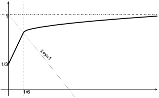
Figure 1: The graph of $\gamma$ (the bold line) in the case $p=3$, $\alpha=1$. Note that $\gamma$ is linear on $[0,1/6]$ and solves (7) on $(1/6,\infty)$.

Let $H\mathchoice{\nobreak\,\colon}{\nobreak\,\colon}{\nobreak\,\colon\;}{\nobreak\,\colon\;}[((\alpha+1)p)^{-1},\infty)\to[1,\infty)$ be given by $H(x)=x+\gamma(x)$ and let $h$ be the inverse to $H$. Clearly, we have

$$x-1\leq h(x)\leq x,\qquad x\geq 1.$$ (13)

We conclude this section by providing a formula for $h^{\prime}$ to be used later. As

$$h^{\prime}(x)=\frac{1}{H^{\prime}(h(x))}=\frac{1}{1+\gamma^{\prime}(h(x))},\qquad x>1,$$ (14)

it can be derived that, in view of (7),

$$h^{\prime}(x)=\frac{1+((\alpha+1)p)^{p}(p-1)(h(x)-x+1)h(x)^{p-1}}{((\alpha+1)p)^{p}(p-1)(h(x)-x+1)h(x)^{p-2}x}.$$ (15)

3 The special function

Throughout this section, $\alpha\in(0,1]$ and $p\geq 2$ are fixed. Let $S$ denote the strip $[0,\infty)\times[-1,1]$. Consider the following subsets of $S$.

$$D_{0} = \{(x,y)\in S\mathchoice{\nobreak\,\colon}{\nobreak\,\colon}{\nobreak\,\colon\;}{\nobreak\,\colon\;}|y|\leq\gamma(x)\},$$

$$D_{1} = \{(x,y)\in S\mathchoice{\nobreak\,\colon}{\nobreak\,\colon}{\nobreak\,\colon\;}{\nobreak\,\colon\;}|y|>\gamma(x),x+|y|\leq 1\},$$

$$D_{2} = \{(x,y)\in S\mathchoice{\nobreak\,\colon}{\nobreak\,\colon}{\nobreak\,\colon\;}{\nobreak\,\colon\;}|y|>\gamma(x),x+|y|>1\}.$$

Introduce the function $u\mathchoice{\nobreak\,\colon}{\nobreak\,\colon}{\nobreak\,\colon\;}{\nobreak\,\colon\;}S\to\mathbb{R}$ by

$$u(x,y)=\cases{1-[(\alpha+1)p]^{p}x^{p}&\quad\mbox{on }$D_{0}$,\cr 1-\biggl{(}{\displaystyle\frac{px+p|y|-1}{p-1}}\biggr{)}^{p-1}\bigl{[}p\bigl{(}p(\alpha+1)-1\bigr{)}x-p|y|+1\bigr{]}&\quad\mbox{on }$D_{1}$,\cr 1-[(\alpha+1)p]^{p}h(x+|y|)^{p-1}[px-(p-1)h(x+|y|)]&\quad\mbox{on }$D_{2}$.}$$

Let $U\mathchoice{\nobreak\,\colon}{\nobreak\,\colon}{\nobreak\,\colon\;}{\nobreak\,\colon\;}[0,\infty)\times\mathbb{R}\times(0,\infty)\to\mathbb{R}$ be given by

$$U(x,y,z)=(|y|\vee z)^{p}u\biggl{(}\frac{x}{|y|\vee z},\frac{y}{|y|\vee z}\biggr{)}.$$

As we will see below, the function $U$ is the key to the inequality (5). Let us study the properties of this function.

Lemma 3.1

The function $U$ is of class $C^{1}$. Furthermore, there exists an absolute constant $K$ such that, for all $x>0,y\in\mathbb{R},z>0,$ we have

$$U(x,y,z)\leq K(x+|y|+z)^{p}$$ (16)

and

$$U_{x}(x,y,z)\leq K(x+|y|+z)^{p-1},\qquad U_{x}(x,y,z)\leq K(x+|y|+z)^{p-1}.$$ (17)

[Proof.] The continuity of the partial derivatives can be verified readily. The inequality (16) is evident for those $(x,y,z)$, for which $(\frac{x}{|y|\vee z},\frac{y}{|y|\vee z})\in D_{0}\cup D_{1}$; for the remaining $(x,y,z),$ it suffices to use (13). Finally, the inequality (17) is clear if $(\frac{x}{|y|\vee z},\frac{y}{|y|\vee z})\in D_{0}\cup D_{1}$. For the remaining points one applies (13) and (14), the latter inequality implying $h^{\prime}<1$.

Now let us deal with the following majorization property.

Lemma 3.2

For any $(x,y,z)\in[0,\infty)\times\mathbb{R}\times(0,\infty)$, we have

$$U(x,y,z)\geq(|y|\vee z)^{p}-[(\alpha+1)p]^{p}x^{p}.$$ (18)

[Proof.] The inequality is equivalent to $u(x,y)\geq 1-[(\alpha+1)p]^{p}x^{p}$ and we need to establish it only on $D_{1}$ and $D_{2}$. On $D_{1}$, the substitutions $X=px$ and $Y=p|y|-1$ (note that $Y\geq 0$) transform it into

$$(\alpha+1)^{p}X^{p}\geq\biggl{(}{\frac{X+Y}{p-1}}\biggr{)}^{p-1}\bigl{[}\bigl{(}p(\alpha+1)-1\bigr{)}X-Y\bigr{]}.$$

This inequality is valid for all non-negative $X$, $Y$. To see this, observe that by homogeneity we may assume $X+Y=1$, and then the estimate reads

$$F(X):=(\alpha+1)^{p}X^{p}-(p-1)^{-p+1}[p(\alpha+1)X-1]\geq 0,\qquad X\in[0,1].$$

Now it suffices to note that $F$ is convex on $[0,1]$ and satisfies

$$F\biggl{(}\frac{1}{(p-1)(\alpha+1)}\biggr{)}=F^{\prime}\biggl{(}\frac{1}{(p-1)(\alpha+1)}\biggr{)}=0.$$

It remains to show the majorization on $D_{2}$. It is dealt with in a similar manner: Setting $s=x+|y|>1$, we see that (18) is equivalent to

$$G(x):=x^{p}-h(s)^{p-1}[px-(p-1)h(s)]\geq 0,\qquad s-1<x<h(s).$$

It is easily verified that $G$ is convex and satisfies $G(h(s))=G^{\prime}(h(s))=0$. This completes the proof of (18).

The main property of the function $U$ is the concavity along the lines of slope belonging to $[-1,1]$.

Lemma 3.3

For fixed $y,z$ satisfying $z>0$, $|y|\leq z$, and any $a\in[-1,1]$, the function $\Phi=\Phi_{y,z,a}\mathchoice{\nobreak\,\colon}{\nobreak\,\colon}{\nobreak\,\colon\;}{\nobreak\,\colon\;}[0,\infty)\to\mathbb{R}$ given by

$$\Phi(t)=U(t,y+at,z)$$

is concave.

Before we turn to the proof, let us first establish some useful consequences.

Corollary 3.4

(i) The function $U$ has the following property: For any $x,y,z,k_{x},k_{y}$ such that $x,x+k_{x}\geq 0$, $z>0$, $|y|\leq z$ and $|k_{y}|\leq|k_{x}|,$ we have

$$U(x+k_{x},y+k_{y},z)\leq U(x,y,z)+U_{x}(x,y,z)k_{x}+U_{y}(x,y,z)k_{y}$$ (19)

(for $x=0,$ we replace $U_{x}(0,y,z)$ by right-sided derivative $U_{x}(0+,y,z)$).

(ii) For any $x\geq 1,$ we have

$$U(x,1,1)\leq 0.$$ (20)

[Proof.] (i) This follows immediately.

(ii) We have $\Phi_{0,1,x^{-1}}(0)=U(0,0,1)=1$ and $\Phi_{0,1,x^{-1}}(((\alpha+1)p)^{-1})=U(((\alpha+1)p)^{-1},\break x^{-1}((\alpha+1)p)^{-1},1)=0$, since $(((\alpha+1)p)^{-1},x^{-1}((\alpha+1)p)^{-1},1)\in D_{0}$. Since $x\geq 1>((\alpha+1)p)^{-1}$, the lemma above gives $U(x,1,1)=\Phi_{0,1,x^{-1}}(x)\leq 0.$

Proof of Lemma 3.3 By homogeneity, we may assume $z=1$. As $\Phi$ is of class $C^{1}$, it suffices to verify that $\Phi^{\prime\prime}(t)\leq 0$ for those $t$, for which $(t,y+at)$ lies in the interior of $D_{0}$, $D_{1}$, $D_{2}$ or outside the strip $S$. Since $U(x,y,z)=U(x,-y,z)$, we may restrict ourselves to the case $y+at\geq 0$. If $(t,y+at)$ belongs to $D_{0}^{o}$, the interior of $D_{0}$, then $\Phi^{\prime\prime}(t)=-[(\alpha+1)p]^{p}\cdot p(p-1)t^{p-2}<0$, while for $(t,y+at)\in D_{1}^{o}$ we have

$$\Phi^{\prime\prime}(t)=-\frac{p^{3}(pt+p(y+at)-1)^{p-3}(1+a)}{(p-1)^{p-2}}(I_{1}+I_{2}),$$

where

$$I_{1} = pt\bigl{[}(p-2)(1+a)\bigl{(}p(\alpha+1)-1\bigr{)}+2\bigl{(}p(\alpha+1)-1-a\bigr{)}\bigr{]}\geq 0,$$

$$I_{2} = \bigl{(}p(y+at)-1\bigr{)}(2\alpha+1-a)\geq 0.$$

The remaining two cases are a bit more complicated. If $(t,y+at)\in D_{2}^{o}$, then

$$\frac{\Phi^{\prime\prime}(t)}{Cp(1+a)^{2}}=J_{1}+J_{2}+J_{3},$$

where

$$J_{1} = h(t+y+at)^{p-2}h^{\prime\prime}(t+y+at)[h(t+y+at)-t],$$

$$J_{2} = h(t+y+at)^{p-3}[h^{\prime}(t+y+at)]^{2}[(p-1)h(t+y+at)-(p-2)t],$$

$$J_{3} = -\frac{2}{a+1}h(t+y+at)^{p-2}h^{\prime}(t+y+at).$$

Now if we change $y$ and $t,$ keeping $s=t+y+at$ fixed, then $J_{1}+J_{2}+J_{3}$ is a linear function of $t\in[s-1,h(s)]$. Therefore, to prove it is non-positive, it suffices to verify this for $t=h(s)$ and $t=s-1$. For $t=h(s)$, we have

$$J_{1}+J_{2}+J_{3}=h(s)^{p-2}h^{\prime}(s)\biggl{[}h^{\prime}(s)-\frac{2}{a+1}\biggr{]}\leq 0,$$

since $0\leq h^{\prime}(s)\leq 1$ (see (14)). If $t=s-1$, rewrite (15) in the form

$$Cs\bigl{(}h(s)+1-s\bigr{)}h(s)^{p-2}h^{\prime}(s)=1+C\bigl{(}h(s)+1-s\bigr{)}h(s)^{p-1}$$

and differentiate both sides; as a result, we obtain

$$Cs\biggl{[}J_{1}+J_{2}+J_{3}+h(s)^{p-2}h^{\prime}(s)\biggl{(}\frac{2}{a+1}-1\biggr{)}\biggr{]}$$

$$\quad=Ch(s)^{p-2}\bigl{[}\bigl{(}h^{\prime}(s)-1\bigr{)}h(s)+(p-2)\bigl{(}h(s)+1-s\bigr{)}h^{\prime}(s)\bigr{]}.$$

As $h^{\prime}\geq 0$ and $2/(a+1)\geq 1$, we will be done if we show the right-hand side is non-positive. This is equivalent to

$$h^{\prime}(s)\bigl{[}h(s)+(p-2)\bigl{(}h(s)+1-s\bigr{)}\bigr{]}\leq h(s).$$

Now use (14) and substitute $h(s)=r$, noting that $h(s)+1-s=1-\gamma(r)$, to obtain

$$r+(p-2)\bigl{(}1-\gamma(r)\bigr{)}\leq r\bigl{(}1+\gamma^{\prime}(r)\bigr{)},$$

or $r\gamma^{\prime}(r)\geq(p-2)(1-\gamma(r))$, which is (12).

Finally, suppose that $y+at>1$. For such $t$ we have $\Phi(t)=(y+at)^{p}u(t/(y+at),1)$, hence, setting $X=t/(y+t),Y=y+at$, we easily check that $\Phi^{\prime\prime}(t)$ equals

$$Y^{p-2}[p(p-1)a^{2}u(X,1)+2a(p-1)(1-aX)u_{x}(X,1)+(1-aX)^{2}u_{xx}(X,1)].$$

First let us derive the expressions for the partial derivatives. Using (15), we have

$$u_{x}(X,1) = \frac{p}{X+1}\bigl{[}1+C\bigl{(}h(X+1)-X\bigr{)}h(X+1)^{p-1}\bigr{]}-\frac{Cph(X+1)^{p-1}}{p-1},$$

$$u_{xx}(X,1) = \frac{p(p-1)}{(X+1)^{2}}\bigl{[}1+C\bigl{(}h(X+1)-X\bigr{)}h(X+1)^{p-1}\bigr{]}$$

$${}-\frac{Cph(X+1)^{p-1}}{X+1}-\frac{Cph(X+1)^{p-2}h^{\prime}(X+1)}{X+1}.$$

Now it can be checked that

$$\Phi^{\prime\prime}(t)Y^{2-p}/p=K_{1}+K_{2}+K_{3},$$

where

$$K_{1} = (p-1)\biggl{(}\frac{a+1}{X+1}\biggr{)}^{2}\bigl{[}1+C\bigl{(}h(X+1)-X\bigr{)}h(X+1)^{p-1}\bigr{]},$$

$$K_{2} = -\frac{Ch(X+1)^{p-1}}{X+1}(1+2a-a^{2}X),$$

$$K_{3} = -\biggl{(}\frac{1-aX}{X+1}\biggr{)}^{2}\cdot\frac{1+C(h(X+1)-X)h(X+1)^{p-1}}{h(X+1)-X}$$

$$\leq -\biggl{(}\frac{1-aX}{X+1}\biggr{)}^{2}\cdot Ch(X+1)^{p-1}.$$

We may write

$$K_{2}+K_{3} \leq -\frac{Ch(X+1)^{p-1}}{(X+1)^{2}}[(1+2a-a^{2}X)(X+1)+(1-aX)^{2}]$$

$$= -\frac{Ch(X+1)^{p-1}(a+1)}{(X+1)^{2}}[2+X(1-a)]\leq-\biggl{(}\frac{a+1}{X+1}\biggr{)}^{2}Ch(X+1)^{p-1},$$

where, in the last passage, we used $a\leq 1$. On the other hand, as $h$ is non-decreasing, we have

$$1=\frac{Ch(1)^{p}}{p-1}\leq\frac{Ch(X+1)^{p-1}h(1)}{p-1}.$$

Moreover, since $x\mapsto h(x+1)-x$ is non-increasing (see (14)), we have $h(X+1)-X\leq h(1)$. Combining these two facts, we obtain

$$K_{1} \leq (p-1)\biggl{(}\frac{a+1}{X+1}\biggr{)}^{2}[1+Ch(1)h(X+1)^{p-1}]$$

$$\leq \biggl{(}\frac{a+1}{X+1}\biggr{)}^{2}Ch(X+1)^{p-1}[h(1)+(p-1)h(1)]$$

$$\leq \biggl{(}\frac{a+1}{X+1}\biggr{)}^{2}Ch(X+1)^{p-1},$$

as $ph(1)=(\alpha+1)^{-1}\leq 1$. This implies $K_{1}+K_{2}+K_{3}\leq 0$ and completes the proof.

The final property we will need is the following.

Lemma 3.5

For any $x,y,z$ such that $x\geq 0$, $z>0$ and $|y|\leq z,$ we have

$$U_{x}(x,y,z)\leq-\alpha|U_{y}(x,y,z)|$$ (21)

(if $x=0$, then $U_{x}$ is replaced by a right-sided derivative).

[Proof.] It suffices to show that for fixed $y,z$, $|y|\leq z$, and $a\in[-\alpha,\alpha]$, the function $\Phi=\Phi_{y,z,a}\mathchoice{\nobreak\,\colon}{\nobreak\,\colon}{\nobreak\,\colon\;}{\nobreak\,\colon\;}[0,\infty)\to\mathbb{R}$ given by $\Phi(t)=U(t,y+at,z)$ is non-increasing. Since $\alpha\leq 1$, we know from the previous lemma that $\Phi$ is concave. Hence all we need is $\Phi^{\prime}(0+)\leq 0$. By symmetry, we may assume $y\geq 0$. If $y\leq 1/p$, then the derivative equals $0$; in the remaining case, we have

$$\Phi^{\prime}(0+)=-\frac{p^{2}(py-1)^{p-1}}{(p-1)^{p-1}}(\alpha-a)\leq 0.$$

4 The proof of (5)

First let us observe that it suffices to show (5) for strictly positive $\alpha$. This is an immediate consequence of the fact that $\alpha$-strong subordination implies $\alpha^{\prime}$-strong subordination for $\alpha<\alpha^{\prime}$.

Suppose $f$, $g$ are as in Theorem 1.4. We may restrict ourselves to the case $\|f\|_{p}<\infty$. Hence, by Choi’s inequality (2), we have $\|g\|_{p}<\infty$. It suffices to show that for any $n=0,1,2,\ldots$ we have

$$\mathbb{E}[(g_{n}^{*})^{p}-(\alpha+1)^{p}p^{p}f_{n}^{p}]\leq 0.$$

Clearly, we may assume that $\mathbb{P}(g_{0}>0)=1$, simply replacing $f$, $g$ by $f+\varepsilon$, $g+\varepsilon$ if necessary (here $\varepsilon$ is a small positive number). In particular, this implies $f_{0}>0$ almost surely. In view of the majorization (18), we will be done if we show that the expectation $\mathbb{E}U(f_{n},g_{n},g_{n}^{*})$ is non-positive for any $n$. As a matter of fact, we will show more; namely, that the process $(U(f_{n},g_{n},g_{n}^{*})_{n\geq 0})$ is a supermartingale and $\mathbb{E}U(f_{0},g_{0},g_{0}^{*})\leq 0$.

To this end, fix $n\geq 1$ and observe that $g^{*}_{n}\leq|g_{0}|+|g_{1}|+\cdots+|g_{n}|$, so $g^{*}_{n}$ belongs to $L^{p}$. Thus, by Lemma 3.1 and Hölder’s inequality, the variables $U(f_{n},g_{n},g_{n}^{*})$, $U_{x}(f_{n-1},g_{n-1},g_{n-1}^{*})\,\mathrm{d}f_{n}$ and $U_{y}(f_{n-1},g_{n-1},g_{n-1}^{*})\,\mathrm{d}g_{n}$ are integrable. Moreover, by definition of $U$ and the inequality (19),

$$\mathbb{E}(U(f_{n},g_{n},g_{n}^{*})|\mathcal{F}_{n-1}) = \mathbb{E}(U_{n}(f_{n},g_{n},g_{n-1}^{*})|\mathcal{F}_{n-1})$$

$$= \mathbb{E}\bigl{(}U(f_{n-1}+\mathrm{d}f_{n},g_{n-1}+\mathrm{d}g_{n},g_{n-1}^{*})|\mathcal{F}_{n-1}\bigr{)}$$

$$\leq \mathbb{E}[U(f_{n-1},g_{n-1},g_{n-1}^{*})+U_{x}(f_{n-1},g_{n-1},g_{n-1}^{*})\,\mathrm{d}f_{n}$$

$$\hskip 8.0pt{}+U_{y}(f_{n-1},g_{n-1},g_{n-1}^{*})\,\mathrm{d}g_{n}|\mathcal{F}_{n-1}]$$

$$\leq U(f_{n-1},g_{n-1},g_{n-1}^{*}).$$

The latter inequality is the consequence of the following. By (21) and the submartingale property of $f$,

$$\mathbb{E}(U_{x}(f_{n-1},g_{n-1},g_{n-1}^{*})\,\mathrm{d}f_{n}|\mathcal{F}_{n-1}) = U_{x}(f_{n-1},g_{n-1},g_{n-1}^{*})\mathbb{E}(\mathrm{d}f_{n}|\mathcal{F}_{n-1})$$

$$\leq -\alpha|U_{y}(f_{n-1},g_{n-1},g_{n-1}^{*})|\mathbb{E}(\mathrm{d}f_{n}|\mathcal{F}_{n-1})$$

$$\leq -U_{y}(f_{n-1},g_{n-1},g_{n-1}^{*})\mathbb{E}(\mathrm{d}g_{n}|\mathcal{F}_{n-1})$$

$$= -\mathbb{E}(U_{y}(f_{n-1},g_{n-1},g_{n-1}^{*})\,\mathrm{d}g_{n}|\mathcal{F}_{n-1}),$$

where the second inequality is due to $\alpha$-domination.

To complete the proof, it suffices to show that $\mathbb{E}U(f_{0},g_{0},g_{0}^{*})\leq 0$. However, $U(f_{0},g_{0},g_{0}^{*})=U(f_{0},g_{0},g_{0})=g_{0}^{p}U(f_{0}/g_{0},1,1)$ almost surely and the estimate follows from Corollary 3.4(ii).

5 Sharpness

We start with inequality (4) and restrict ourselves to the case when $g$ is a $\pm 1$ transform of $f$. Suppose the best constant in this estimate equals $\beta>0$. This implies the existence of a function $W\mathchoice{\nobreak\,\colon}{\nobreak\,\colon}{\nobreak\,\colon\;}{\nobreak\,\colon\;}\mathbb{R}\times\mathbb{R}\times[0,\infty)\times[0,\infty)\to\mathbb{R},$ which satisfies the following properties:

$$W(1,1,1,1) \leq 0,$$ (22)

$$W(x,y,z,w) = W(x,y,|x|\vee z,|y|\vee w),\qquad\mbox{if }x,y\in\mathbb{R},w,z\geq 0,$$ (23)

$$(|y|\vee w)^{p}-\beta^{p}(|x|\vee z)^{p} \leq W(x,y,z,w),\qquad\mbox{if }x,y\in\mathbb{R},w,z\geq 0$$ (24)

and, furthermore,

$$aW(x+t_{1},y+\varepsilon t_{1},z,w)+(1-a)W(x+t_{2},y+\varepsilon t_{2},z,w)\leq W(x,y,z,w)$$

(25)

for any $$|x|\leq z,|y|\leq w \varepsilon\in\{-1,1\} a\in(0,1) t_{1},\ t_{2} at_{1}+(1-a)t_{2}=0$$, , and with .

Indeed, one puts

$$W(x,y,z,w)=\sup\{\mathbb{E}(g_{n}^{*}\vee w)^{p}-\beta^{p}\mathbb{E}(f_{n}^{*}\vee z)^{p}\},$$ (26)

where the supremum is taken over all integers $n$ and all martingales $f$, $g$ satisfying $\mathbb{P}((f_{0},g_{0})=(x,y))=1$ and $\mathrm{d}f_{k}=\pm\,\mathrm{d}g_{k}$, $k=1,2,\ldots$ (see [11] for details). This formula allows us to assume that $W$ is homogeneous: $W(tx,ty,tz,tw)=tW(x,y,z,w)$ for all $x,y\in\mathbb{R}$, $z,w\geq 0$ and $t>0$.

Now the idea is to exploit the above properties of $W$ to get $\beta\geq p$. To this end, let $\delta$ be a small number belonging to $(0,1/p)$. By (5) applied to $x=0$, $y=w=1$, $z=\delta/(1+2\delta)$, $\varepsilon=1$ and $t_{1}=\delta$, $t_{2}=-1/p$, we obtain

$$W\biggl{(}0,1,\frac{\delta}{1+2\delta},1\biggr{)} \geq \frac{p\delta}{1+p\delta}W\biggl{(}-\frac{1}{p},1-\frac{1}{p},\frac{\delta}{1+2\delta},1\biggr{)}$$

$${}+\frac{1}{1+p\delta}W\biggl{(}\delta,1+\delta,\frac{\delta}{1+2\delta},1+\delta\biggr{)}.$$

Now, by (23) and (24),

$$W\biggl{(}-\frac{1}{p},1-\frac{1}{p},\frac{\delta}{1+2\delta},1\biggr{)}=W\biggl{(}-\frac{1}{p},1-\frac{1}{p},\frac{1}{p},1\biggr{)}\geq 1-\biggl{(}\frac{\beta}{p}\biggr{)}^{p}.$$ (28)

Furthermore, by (23),

$$W\biggl{(}\delta,1+\delta,\frac{\delta}{1+2\delta},1+\delta\biggr{)}=W(\delta,1+\delta,\delta,1+\delta),$$

which, by (5) (with $x=z=\delta$, $y=w=1+\delta$, $\varepsilon=-1$ and $t_{1}=-\delta$, $t_{2}=\frac{1}{p}+\delta(\frac{1}{p}-1)$), can be bounded from below by

$$\frac{p\delta}{1+\delta}W\biggl{(}\frac{1+\delta}{p},1-\frac{1}{p}+\delta\biggl{(}2-\frac{1}{p}\biggr{)},\delta,1+\delta\biggr{)}+\frac{1+\delta-p\delta}{1+\delta}W(0,1+2\delta,\delta,1+\delta).\$$

Using (24), we get

$$W\biggl{(}\frac{1+\delta}{p},1-\frac{1}{p}+\delta\biggl{(}2-\frac{1}{p}\biggr{)},\delta,1+\delta\biggr{)}\geq(1+\delta)^{p}\biggl{[}1-\biggl{(}\frac{\beta}{p}\biggr{)}^{p}\biggr{]}.$$

Furthermore, by (23) and the homogeneity of $W$,

$$W(0,1+2\delta,\delta,1+\delta)=W(0,1+2\delta,\delta,1+2\delta)=(1+2\delta)^{p}W\biggl{(}0,1,\frac{\delta}{1+2\delta},1\biggr{)}.$$

Now plug all the above estimates into (5) to get

$$W\biggl{(}0,1,\frac{\delta}{1+2\delta},1\biggr{)}\biggl{[}1-\frac{(1+\delta-p\delta)(1+2\delta)^{p}}{(1+\delta)(1+p\delta)}\biggr{]}$$

(29)

$$\quad\geq\frac{p\delta}{1+p\delta}\biggl{[}1-\biggl{(}\frac{\beta}{p}\biggr{)}^{p}\biggr{]}\bigl{(}1+(1+\delta)^{p-1}\bigr{)}.$$

Now it follows from the definition (26) of $W$ that

$$W\biggl{(}0,1,\frac{\delta}{1+2\delta},1\biggr{)}\leq W(0,1,0,1).$$

Furthermore, one easily checks that the function

$$F(s)=1-\frac{(1+s-ps)(1+2s)^{p}}{(1+s)(1+ps)},\qquad s>-\frac{1}{p},$$

satisfies $F(0)=F^{\prime}(0)=0$. Hence

$$1-\biggl{(}\frac{\beta}{p}\biggr{)}^{p}\leq\frac{W(0,1,0,1)\cdot F(\delta)\cdot(1+p\delta)}{p\delta(1+(1+\delta)^{p-1})}$$

and letting $\delta\to 0$ yields $1-(\frac{\beta}{p})^{p}\leq 0$, or $\beta\geq p$.

The reasoning for the inequality (6) is essentially the same: suppose the best constant in the estimate equals $\gamma>0$. Introduce the function $V\mathchoice{\nobreak\,\colon}{\nobreak\,\colon}{\nobreak\,\colon\;}{\nobreak\,\colon\;}[0,\infty)\times\mathbb{R}\times[0,\infty)\times[0,\infty)\to\mathbb{R}$ by

$$V(x,y,z,w)=\sup\{\mathbb{E}(g_{n}^{*}\vee w)^{p}-\gamma^{p}\mathbb{E}(f_{n}^{*}\vee z)^{p}\},$$

where the supremum is taken over all integers $n$, all non-negative submartingales $f$ and all integrable sequences $g$ satisfying $\mathbb{P}((f_{0},g_{0})=(x,y))=1$ and, for $k=1,2,\ldots,$

$$|\mathrm{d}f_{k}|\geq|\mathrm{d}g_{k}|,\qquad\alpha\mathbb{E}(\mathrm{d}f_{k}|\mathcal{F}_{k-1})\geq|\mathbb{E}(\mathrm{d}g_{k}|\mathcal{F}_{k-1})|$$

with probability $1$. We see that $V$ is homogeneous and satisfies the properties analogous to (22)–(5) (with obvious changes: in (23) and (24) one must assume $x\geq 0$; in (24) the number $\beta$ is replaced by $\gamma;$ and, in (5), we impose $x,x+t_{1},x+t_{2}\geq 0$). In addition, there is an extra property of $V$, which corresponds to the fact that we deal with the inequality for submartingales:

$$V(x+d,y+\alpha d,z,w)\leq V(x,y,z,w),\qquad\mbox{if }x\geq 0,y\in\mathbb{R},w,z\geq 0,d\geq 0.$$ (30)

Now fix $\delta\in(0,1/p)$ and apply this property with $x=0$, $y=w=1$, $z=\delta/(1+(\alpha+1)p)$, $d=\delta$ and then use (23) to obtain

$$V\biggl{(}0,1,\frac{\delta}{1+(\alpha+1)\delta},1\biggr{)} \geq V\biggl{(}\delta,1+\alpha\delta,\frac{\delta}{1+(\alpha+1)\delta},1\biggr{)}$$

$$= V(\delta,1+\alpha\delta,\delta,1+\alpha\delta).$$

Using (23), (24) and (5) as above, we have

$$V(\delta,1+\alpha\delta,\delta,1+\alpha\delta) \geq \frac{\delta(\alpha+1)p}{1+\alpha\delta}(1+\alpha\delta)^{p}\biggl{[}1-\biggl{(}\frac{\gamma}{(\alpha+1)p}\biggr{)}^{p}\biggr{]}$$

$${}+\frac{1+\alpha\delta-\delta(\alpha+1)p}{1+\alpha\delta}\bigl{(}1+(\alpha+1)\delta\bigr{)}^{p}V\biggl{(}0,1,\frac{\delta}{1+(\alpha+1)\delta},1\biggr{)},$$

which, combined with (5), gives

$$V\biggl{(}0,1,\frac{\delta}{1+(\alpha+1)\delta},1\biggr{)}\biggl{[}1-\frac{1+\alpha\delta-\delta(\alpha+1)p}{1+\alpha\delta}\bigl{(}1+(\alpha+1)\delta\bigr{)}^{p}\biggr{]}$$

$$\quad\geq\delta(\alpha+1)p(1+\alpha\delta)^{p-1}\biggl{[}1-\biggl{(}\frac{\gamma}{(\alpha+1)p}\biggr{)}^{p}\biggr{]}.$$

Now it suffices to use

$$V\biggl{(}0,1,\frac{\delta}{1+(\alpha+1)\delta},1\biggr{)}\leq V(0,1,0,1)$$

and the fact that the function

$$G(s)=1-\frac{1+\alpha s-s(\alpha+1)p}{1+\alpha s}\bigl{(}1+(\alpha+1)s\bigr{)}^{p},\qquad s>-1/\alpha,$$

satisfies $G(0)=G^{\prime}(0)=0$, to obtain

$$1-\biggl{(}\frac{\gamma}{(\alpha+1)p}\biggr{)}^{p}\leq\frac{V(0,1,0,1)G(\delta)}{\delta(\alpha+1)p(1+\alpha\delta)^{p-1}}.$$

Letting $\delta\to 0$ gives $1-(\frac{\gamma}{(\alpha+1)p})^{p}\leq 0$, or $\gamma\geq(\alpha+1)p$. This completes the proof.

6 Inequalities for stochastic integrals and Itô processes

In this section we present applications of the results above. Theorem 1.4 in the special case $\alpha=1$ yields an interesting inequality for the stochastic integrals. Suppose $(\Omega,\mathcal{F},\mathbb{P})$ is a complete probability space, filtered by a non-decreasing right-continuous family $(\mathcal{F}_{t})_{t\geq 0}$ of sub-$\sigma$-fields of $\mathcal{F}$. In addition, let $\mathcal{F}_{0}$ contain all the events of probability $0$. Suppose $X=(X_{t})_{t\geq 0}$ is an adapted non-negative right-continuous submartingale with left limits and let $Y$ be the Itô integral of $H$ with respect to $X$,

$$Y_{t}=H_{0}X_{0}+\int_{(0,t]}H_{s}\,\mathrm{d}X_{s},\qquad t\geq 0.$$

Here $H$ is a predictable process with values in $[-1,1]$. Denote $\|X\|_{p}=\sup_{t\geq 0}\|X_{t}\|_{p}$ and $X^{*}=\sup_{t\geq 0}|X_{t}|.$ We will establish the following extension of Theorem 1.4.

Theorem 6.1

Under the above conditions, we have, for any $p\geq 2$,

$$\|Y^{*}\|_{p}\leq 2p\|X\|_{p},$$ (32)

and the constant $2p$ is the best possible. It is already the best possible in the weaker estimate

$$\|Y^{*}\|_{p}\leq 2p\|X^{*}\|_{p}.$$

[Proof.] The constant $2p$ is optimal even in the discrete-time setting, so all we need is to show (32). This is a consequence of the approximation results of Bichteler [3]. We proceed as follows: Consider the family Y of all processes $Y$ of the form

$$Y_{t}=H_{0}X_{0}+\sum_{k=1}^{n}h_{k}[X_{\tau_{k}\wedge t}-X_{\tau_{k-1}\wedge t}],$$ (33)

where $n$ is a positive integer, $h_{k}$ belongs to $[-1,1]$ and the stopping times $\tau_{k}$ take only a finite number of finite values, with $0=\tau_{0}\leq\tau_{1}\leq\cdots\leq\tau_{n}$. Let

$$f=(X_{\tau_{0}},X_{\tau_{1}},\ldots,X_{\tau_{n}},X_{\tau_{n}},\ldots)$$

and let $g$ be the transform of $f$ by $(H_{0},h_{1},h_{2},\ldots,h_{n},0,0,\ldots)$. In virtue of Doob’s optional sampling theorem, $f$ is a submartingale. Therefore, by Theorem 1.4, if $\tau_{n}\leq t$ almost surely, then for $Y$ as in (33),

$$\|Y_{t}^{*}\|_{p}=\|g_{n}^{*}\|_{p}\leq 2p\|f_{n}\|_{p}\leq 2p\|X_{t}\|_{p}.$$

Now we have that $X$ and $H$ satisfy the conditions of Proposition 4.1 of Bichteler [3]. Thus by (2) of that proposition, if $Y$ is as in the statement of the theorem above, then there is a sequence $(Y^{j})$ of elements of Y such that $\lim_{j\to\infty}(Y^{j}-Y)^{*}=0$ almost surely. Hence, by Fatou’s lemma,

$$\|Y^{*}_{t}\|_{p}\leq 2p\|X_{t}\|_{p}.$$

Now take $t\to\infty$ to complete the proof.

The result above can be further strengthened. Assume that $X$ is a non-negative submartingale and $X=X_{0}+M+A$ stands for its Doob–Meyer decomposition, uniquely determined by the condition that $A$ is predictable. Let $\alpha\in[0,1]$ be fixed and suppose $\phi$, $\psi$ are predictable processes satisfying $|\phi_{s}|\leq 1$ and $|\psi_{s}|\leq\alpha$ for all $s$. Consider the Itô process $Y$ such that $|Y_{0}|\leq X_{0}$ and

$$Y_{t}=Y_{0}+\int_{0+}^{t}\phi_{s}\,\mathrm{d}M_{s}+\int_{0+}^{t}\psi_{s}\,\mathrm{d}A_{s}$$

for all $t\geq 0$. We have the following sharp bound.

Theorem 6.2

For $X$, $Y$ as above, we have

$$\|Y^{*}\|_{p}\leq(\alpha+1)p\|X\|_{p}$$

and the inequality is sharp. So is the weaker estimate

$$\|Y^{*}\|_{p}\leq(\alpha+1)p\|X^{*}\|_{p}.$$

This result can be established using essentially the same approximation arguments as above; we omit the details. We would only like to mention here that there is an alternative way of proving Theorems 6.1 and 6.2, based on Itô’s formula applied to the function $u$ (as the function is not of class $C^{2}$, one needs some additional “smoothing” arguments to overcome this difficulty). See [19] or [20] for similar reasoning.

References

[1]
Bañuelos, R. and Bogdan, K. (2007). Lévy processes
and Fourier multipliers. J. Funct. Anal.250 197–213.
MR2345912
[2]
Bañuelos, R. and Wang, G. (1995). Sharp inequalities
for martingales with applications to the Beurling–Ahlfors and Riesz
transformations. Duke Math. J.80 575–600.
MR1370109
[3]
Bichteler, K. (1980). Stochastic integration and
-theory of semimartingales. Ann. Probab.9 49–89.
MR0606798
[4]
Bourgain, J. (1983). Some remarks on Banach spaces in
which martingale difference sequences are unconditional. Ark.
Mat.21 163–168.
MR0727340
[5]
Burkholder, D.L. (1981). A geometrical characterization
of Banach spaces in which martingale difference sequences are
unconditional. Ann. Probab.9 997–1011.
MR0632972
[6]
Burkholder, D.L. (1984). Boundary value problems and
sharp inequalities for martingale transforms. Ann. Probab.12 647–702.
MR0744226
[7]
Burkholder, D.L. (1985). An elementary proof of an
inequality of R. E. A. C. Paley. Bull. London Math. Soc.17 474–478.
MR0806015
[8]
Burkholder, D.L. (1989). Differential
subordination of harmonic functions and martingales. In Harmonic Analysis
and Partial Differential Equations (El Escorial, 1987). Lecture Notes
in Mathematics1384 1–23. Berlin: Springer.
MR1013814
[9]
Burkholder, D.L. (1991). Explorations in
martingale theory and its applications. In Ecole d’Eté de Probabilités de Saint-Flour XIX—1989. Lecture Notes in Math.1464 1–66. Berlin: Springer.
MR1108183
[10]
Burkholder, D.L. (1994). Strong differential
subordination and stochastic integration. Ann. Probab.22 995–1025.
MR1288140
[11]
Burkholder, D.L. (1997). Sharp norm comparison of
martingale maximal functions and stochastic integrals. In Proceedings of
the Norbert Wiener Centenary Congress, 1994 (East Lansing, MI, 1994).
Proc. Sympos. Appl. Math.52 343–358. Providence, RI: Amer. Math. Soc.
MR1440921
[12]
Choi, C. (1996). A submartingale inequality. Proc.
Amer. Math. Soc.124 2549–2553.
MR1353381
[13]
Choi, C. (1998). A weak-type inequality of subharmonic
functions. Proc. Amer. Math. Soc.126 1149–1153.
MR1425115
[14]
Choi, C. (1998). A weak-type inequality for
differentially subordinate harmonic functions. Trans. Amer.
Math. Soc.350 2687–2696.
MR1617340
[15]
Hammack, W. (1995). Sharp inequalities for the
distribution of a stochastic integral in which the integrator is a
bounded submartingale. Ann. Probab.23 223–235.
MR1330768
[16]
Osȩkowski, A. (2007). Sharp norm inequalities for
martingales and their differential subordinates. Bull. Polish
Acad. Sci. Math.55 373–385.
MR2369123
[17]
Osȩkowski, A. (2008). Sharp maximal inequality for
stochastic integrals. Proc. Amer. Math. Soc.136
2951–2958.
MR2399063
[18]
Osȩkowski, A. (2008). Sharp LlogL inequalities for
differentially subordinated martingales. Illinois J. Math.52 745–756.
MR2546005
[19]
Osȩkowski, A. (2009). Sharp weak type inequalities
for differentially subordinated martingales. Bernoulli15 871–897.
MR2555203
[20]
Suh, Y. (2005). A sharp weak type inequality
for martingale transforms and other subordinate
martingales. Trans. Amer. Math. Soc.357 1545–1564.
MR2115376
[21]
Wang, G. (1995). Differential subordination and strong
differential subordination for continuous-time martingales and
related sharp inequalities. Ann. Probab.23
522–551.
MR1334160