Masses of subgiant stars from asteroseismology using the coupling strengths of mixed modes

Abstract

Since few decades, asteroseismology, the study of stellar oscillations, enables us to probe the interiors of stars with great precision. It allows stringent tests of stellar models and can provide accurate radii, masses and ages for individual stars. Of particular interest are the mixed modes that occur in subgiant solar-like stars since they can place very strong constraints on stellar ages. Here we measure the characteristics of the mixed modes, particularly the coupling strength, using a grid of stellar models for stars with masses between $0.9$ and $1.5$ $M_{\odot}$. We show that the coupling strength of the $\ell=1$ mixed modes is predominantly a function of stellar mass and appears to be independent of metallicity. This should allow an accurate mass evaluation, further increasing the usefulness of mixed modes in subgiants as asteroseismic tools.

1. Introduction

Asteroseismology allows stringent tests of stellar models and can provide accurate fundamental properties of individual stars. For solar-type stars on the main sequence, the observed oscillations are $p$ modes, for which the restoring force arises from the pressure gradient. These are approximately regularly spaced in frequency, following closely the so-called asymptotic relation (Vandakurov, 1967; Tassoul, 1980; Gough, 1986). However, the oscillations of post-main-sequence stars show departures from this regularity that are due to the presence of mixed modes.

Mixed modes have $p$-mode character in the stellar envelope and $g$-mode character in the core. They occur in evolved stars (subgiants and red giants), in which the large density gradient outside the core effectively divides the star into two coupled cavities. This leads to mode bumping, in which mode frequencies are shifted from their regular spacing and no longer follow the asymptotic relation. Mode bumping in subgiant stars was first observed and modeled in $\eta$ Boo (Kjeldsen et al., 1995, 2003; Christensen-Dalsgaard et al., 1995; Carrier et al., 2005) and $\beta$ Hyi (Bedding et al., 2007; Brandão et al., 2011). More recently, asteroseismic space missions have produced many more examples, including the CoRoT target HD 49835 (Deheuvels et al., 2010) and a growing number of Kepler stars (e.g., Metcalfe et al. 2010; Mathur et al. 2010; Campante et al. 2011).

Mixed modes carry valuable information on the internal structure and evolutionary state of stars. Their frequencies change quickly with time as they undergo avoided crossings (Osaki, 1975; Aizenman et al., 1977), potentially providing stellar ages with a precision down to a few Myr, or a relative uncertainty of $\approx 1\%$ (Metcalfe et al., 2010).
Mixed modes arise from a resonant coupling between $p$ and $g$ modes and can be well represented by a system of coupled oscillators. In this Letter, we use such a representation to model their frequencies in subgiant stars and determine the coupling strength between the modes. We show that the coupling strength depends strongly on stellar mass but only weakly (or not at all) on metallicity, hence lifting the often problematic degeneracy between those two variables.

2. A model for mixed modes

Mixed modes in stars occur when the $p$ and $g$ modes are coupled, which leads to avoided crossings and mode bumping. Deheuvels & Michel (2010a) suggested that an avoided crossing in a subgiant star can be well-represented by a system of $(n-1)$ $p$-mode oscillators, each coupled with a single $g$ mode. This can be modeled by a system of $n$ differential equations, one for each of the $p$ modes and one for the $g$ mode:

$$\frac{d^{2}y_{1}(t)}{dt^{2}} = -\omega_{\pi_{1}}^{2}y_{1}+\alpha_{1,n}y_{n}$$ (1)

$$\vdots$$

$$\frac{d^{2}y_{n-1}(t)}{dt^{2}} = -\omega_{\pi_{n-1}}^{2}y_{n-1}+\alpha_{n-1,n}y_{n}$$

$$\frac{d^{2}y_{n}(t)}{dt^{2}} = -\omega_{\gamma}^{2}y_{n}+\alpha_{1,n}y_{1}+...+\alpha_{n-1,n}y_{n-1}$$

The $y_{i}(t)$ terms are the displacements of the modes and $\alpha_{i,n}$ are the coupling coefficients between the $i$th $p$ mode and the $g$ mode. The frequencies $\omega_{\pi_{i}}$ and $\omega_{\gamma}$ correspond to fictitious, pure $p$ and $g$ modes that would exist if their cavities were not coupled. In order to avoid ambiguity, we follow Aizenman et al. (1977) by referring to these as $\pi$ and $\gamma$ modes, respectively (see also Bedding 2011a).

We seek oscillatory solutions of Eq. 1 with angular frequencies $\Omega=\left\{\omega_{1},\omega_{2},...,\omega_{n}\right\}$, which means we need to solve the following system:

$$\mbox{\boldmath$A$}Y=\Omega^{2}Y,$$ (2)

where $Y=\left\{y_{1},y_{2},...,y_{n}\right\}$ and

$$\mbox{\boldmath$A$}=\left(\begin{array}[]{ccccc}\omega_{\pi_{1}}^{2}&\cdots&0&-\alpha\\ \vdots&\ddots&0&-\alpha\\ 0&\cdots&\omega_{\pi_{n-1}}^{2}&-\alpha\\ -\alpha&\cdots&-\alpha&\omega_{\gamma}^{2}\end{array}\right).$$ (3)

Following Deheuvels & Michel (2010a), we assumed the coupling $\alpha_{i,n}\equiv\alpha$ to be the same between all modes. This is a reasonable assumption provided $\alpha$ varies slowly with frequency, which turns out to be the case in the models we have studied.

In more evolved stars (red giants), the situation is reversed and several $g$-modes may be coupled to a single $p$-mode (Dupret et al., 2009; Christensen-Dalsgaard, 2011; Bedding, 2011a; Stello, 2011). Between these two extremes, one can consider intermediate cases with multiple $g$-modes and $p$-modes (e.g., di Mauro et al., 2011), whose power spectra may become hard to interpret.

For the case of $n=2$, which is a single $\pi$ mode coupling to a $\gamma$ mode, Eq. 2 can be solved analytically to give a pair of solutions (Deheuvels & Michel, 2010a):

$$\omega_{\pm}^{2}=\frac{\omega_{\pi}^{2}+\omega_{\gamma}^{2}}{2}\pm{\textstyle\frac{1}{2}}\sqrt{(\omega_{\pi}^{2}-\omega_{\gamma}^{2})^{2}+4\alpha^{2}}.$$ (4)

The black curves in Figure 1 shows these two solutions in a replicated échelle diagram (Bedding, 2011b).

We note that the coefficient $\alpha$ is not an ideal measure of the coupling strength between $\pi$ and $\gamma$ modes because it varies with frequency and is therefore different for each avoided crossing. A better measure is the frequency separation of the two solutions at the avoided crossing. That is, we focus on the point of resonance by setting $\omega_{\gamma}=\omega_{\pi}$ and measure the frequency difference between the two solutions:

$$\delta\omega_{\gamma}=\omega_{+}-\omega_{-}.$$ (5)

It follows from Eq. 4 that

$$\delta\omega_{\gamma}=\alpha/\omega_{\gamma},$$ (6)

or, in cyclic frequency,

$$\delta\nu_{\gamma}=\delta\omega_{\gamma}/2\pi=\frac{\alpha}{4\pi^{2}\nu_{\gamma}}.$$ (7)

For the case of $n>2$, which involves several $\pi$ modes coupling to a $\gamma$ mode, Eq. 2 can be solved numerically. We find a set of solutions, shown by the red curves in Figure 1 for the case of $n=8$. The value of $\delta\nu_{\gamma}$ is shown by the solid red line.
The minimal separation is almost independent of the number of interacting modes (black and red lines are close to each other at $\omega_{\pi}\simeq\omega_{\gamma}$). The stronger the coupling, the larger the separation.

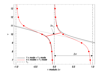
Figure 1.— Replicated échelle diagram showing the effect of the coupling between the $\pi$ and $\gamma$ modes in two configurations: two coupled modes (black), and several coupled modes (red) with $\pi$-modes frequencies spaced by $\Delta\nu$. $\nu_{\gamma}$ is arbitrarily fixed to $10$. Where the $\pi$ and $\gamma$ modes cross, the frequency separation is $\delta\nu_{\gamma}$ (diagonal red line). $\delta\nu_{\gamma}$ is almost independent of $n$, the number of interacting modes.

3. Fitting method

For each avoided crossing we have a sequence of observed frequencies that correspond to the mixed modes. Each observed frequency must satisfy Eq. 2. Provided we have enough observed frequencies, we can determine the elements of the matrix $A$, which gives the $\pi$ and $\gamma$ mode frequencies, and the coupling strength $\alpha$.

To carry out this fitting process robustly, we apply a Bayesian approach (Maximum a Posteriori Approach, hereafter MAP). Assuming a likelihood function $L(\nu_{\rm obs}|\mbox{\boldmath$A$})$, one can regularize this function by penalizing it with a quantity $p(\mbox{\boldmath$A$})$, called the prior, where $\nu_{\rm obs}$ represents the observed frequencies (the data). Using Bayes’ theorem, we write the statistical criteria defining the fit quality that we seek to maximize as

$$\ln[p(\mbox{\boldmath$A$}|\nu_{\rm obs})]=\ln[L(\nu_{\rm obs}|\mbox{\boldmath$A$})]+\ln[p(\mbox{\boldmath$A$})]-\ln[C].$$ (8)

Here, $C$ is a normalization constant and $p(\mbox{\boldmath$A$}|\nu_{\rm obs})$ is the posterior probability (the probability of $A$ given  $\nu_{\rm obs}$).

The linear system in Eq. 2 must be solved at each iteration of the maximization process in order to compare the observed frequencies $\nu_{\rm obs}$ with the calculated frequencies $\nu_{\rm calc}$. The expression we choose to minimize is ${\textstyle\frac{1}{2}}\sum_{i}\left(\nu_{\rm obs}(n)-\nu_{\rm calc}(n)\right)^{2}/\sigma^{2}_{n}$. Thus the log-likelihood is,

$$\ln[L(\nu_{\rm obs}|\mbox{\boldmath$A$})]\propto-{\textstyle\frac{1}{2}}\sum_{n}(\nu_{\rm obs}(n)-\nu_{\rm calc}(n))^{2}/\sigma^{2}_{n}.$$ (9)

where $\sigma_{n}=1$ for model frequencies.

Having defined the likelihood, we must choose expressions for the priors. No priors on $\alpha$ and $\nu_{\gamma}$ were applied and our attention will focus on  $\nu_{\pi_{i}}$. The pseudo-modes $\pi$ and $\gamma$ are expected to behave as pure $p$ and $g$ modes. To a good approximation, the $\pi$-modes should follow the asymptotic relation (Tassoul, 1980):

$$\nu_{\pi}(n)=(n+\frac{\ell}{2}+\epsilon)\Delta\nu-\delta\nu_{0\ell},$$ (10)

where $n$ is the radial order, $\epsilon$ is an offset associated with stellar surface effects, $\Delta\nu$ is the large separation (related to the mean density of the star), and $\delta\nu_{0\ell}$ is sensitive to the core properties. In this Letter, we only consider the case of $\ell=1$ (dipole modes).

Discontinuities inside stars introduce frequency oscillations as a function of $n$, not included in the asymptotic relation. These oscillations are not expected to be significant, say less than a few percent of $\Delta\nu$. Thus the $\pi$-mode frequency variations are expected to be smooth, as seen in the échelle diagram for the $p$-modes of main sequence stars. A way to satisfy this condition is to impose a smoothness condition on some $p$th derivative terms of $\nu_{\pi}(n)$. We note that the second derivative in $n$ of Eq. 10, denoted $\Delta^{2}\nu(n)$, leads to $\Delta^{2}\nu(n)=\frac{\partial^{2}\nu_{\pi}}{\partial n^{2}}\approx 0$. Thus one may limit local strong deviations from a regular pattern by imposing a Gaussian prior on $\Delta^{2}\nu(n)$,

$$p(\Delta^{2}\nu(n))=\frac{1}{\sqrt{2\pi}\sigma_{\Delta^{2}\nu}}\exp\left[-{\textstyle\frac{1}{2}}\left(\frac{\Delta^{2}\nu(n)}{\sigma_{\Delta^{2}\nu}}\right)^{2}\right].$$ (11)

Here, $\sigma_{\Delta^{2}\nu}$ plays the role of a relaxation constraint and must be chosen to ensure enough freedom, but not too much, in order to efficiently smooth the frequency profile. A trial-and-error procedure showed that $\sigma_{\Delta^{2}\nu}\approx 2$ $\mu$Hz offers a good compromise. With such a smoothness condition, the $\pi$-mode deviation from a strictly regular pattern of frequencies is locally described by a second-order polynomial function of $n$, and the solution belongs to the family of spline functions. The smoothness condition acts locally and does not restrict the $\pi$-modes to follow the asymptotic relation, globally.

We define an additional (global) condition, in order to avoid strong departures from Eq.10. We expect the $\ell=0$ modes and $\ell=1$ $\pi$ modes to be distributed along two parallel ridges in the échelle diagram. Hence, the large separation $\Delta\nu$ of the $\ell=0$ mode, is expected to be approximately equal to the large separation $\Delta\nu_{\pi}$ of the $\ell=1$ $\pi$ modes. Thus a second Gaussian prior was applied to the quantity $\Delta\nu_{\pi}-\Delta\nu$, with $\sigma_{\Delta\nu_{\pi}}\approx 1/\sqrt{N}$ $\mu$Hz, $N$ being the number of modes.

4. Results for stellar models

We have applied our method to frequencies of $\ell=1$ modes calculated from stellar models. Models were selected from the grid described in detail by Stello et al. (2009). This grid was generated with the ASTEC code (Christensen-Dalsgaard, 2008) using the simple but fast EFF equation of state (Eggleton et al., 1973), a fixed mixed length parameter at $\alpha_{\rm MLT}=1.8$, and an initial hydrogen abundance of $X=0.7$. The opacities were calculated using the solar mixture (Grevesse & Noels, 1993) and the opacity tables of Rogers & Iglesias (1995) and Kurucz (1991). Rotation, overshooting and diffusion were not included.

Models with masses in the range $0.9$ to $1.5\,M_{\odot}$ were explored with a step size of $0.1\,M_{\odot}$. All models were computed for solar metallicity ($Z=0.017$). In addition, lower and higher metallicities ($Z=0.011$ and $Z=0.028$) were considered for a subset of masses ($1.0\,M_{\odot}$, $1.2\,M_{\odot}$, $1.3\,M_{\odot}$ and $1.5\,M_{\odot}$).

In general, stars have mixed $\ell=1$ modes while still on the main sequence. However, these occur at low frequencies that lie outside the envelope of observable modes. Mode bumping only starts to be detectable once a star has entered the subgiant phase. As discussed in the Introduction, each avoided crossing is associated with a g mode trapped in the core of the star (a $\gamma$ mode; see also Deheuvels & Michel 2010b; Bedding 2011a). The $\gamma$-mode frequencies increase as the star evolves and we tracked each one. As additional avoided crossings appeared at low frequency, they were also incorporated into Eq. 2. In this way, the stellar model was followed during a significant part of the subgiant phase, as shown in the HR diagram in Figure 2. Towards the end of this phase, the frequency patterns became too complex (too few modes between each avoided crossing) and a stable fit was difficult to obtain. We secured reliable results for models with up to three observable avoided crossings, each of them characterized by its frequency $\nu_{\gamma}$, and its coupling strength (measured by $\delta\nu_{\gamma}$ — see Eq. 7).

Figure 3 shows the results, with each panel showing the coupling strength as a function of the avoided crossing frequency. The central frequency of the modes $\nu_{max}$ decreases over time and thus, goes from right to left along a star’s evolution in these diagrams. The systematic error on the determination of $\delta\nu_{\gamma}$ is about $1.5\,\mu$Hz. This uncertainty arises from Eq. 2 not being a perfect representation of the behavior of the frequencies of the stellar models. In Figure 3a we show only the highest-frequency avoided crossing. The different tracks show models with four different masses and three different metallicities. Interestingly, the coupling strength depends strongly on mass (as noted by Deheuvels & Michel 2011) but only weakly on metallicity, if at all. The systematic error prevents us from assessing whether the small variations of the coupling strength are really due to the metallicity. it suggests that we may be able to use the coupling strength to break the degeneracy between mass and metallicity, which is often a problem in asteroseismology.

As mentioned above, $\gamma$ modes frequencies increase as a star evolves and several avoided crossing may enter the range of observable frequencies. In Figure 3b we show $\delta\nu_{\gamma}$ for the first three avoided crossings for evolving models with four different masses. They all have solar metallicity. For a given mass, all three curves closely follow the same path in the diagram (but with a time delay). This confirms that $\delta\nu_{\gamma}$, as defined by Eq. 7, is an excellent measure of the coupling strength between the p- and g-mode cavities.

In Figure 3a and 3b we see rapid changes in the coupling strength at the low-frequency end. This reflects rapid changes in the extent of the evanescent zone that separates the inner g-mode and outer p-mode cavities. Indeed, the coupling strength depends on the extension of this zone, in the sense that a smaller evanescent zone leads to stronger coupling. In Figure 3b the tracks for the different avoided crossings (for a given mass) no longer follow a single path at low frequency. During the transition between the main sequence and the post main sequence stage, the density of the star and thus, the shape of the evanescent zone, vary on very short timescale. Thus the evanescent zone has changed significantly between the times when the first and third avoided crossing pass the same frequency. For the most evolved stars, which means when several $\gamma$ modes have a frequency close to $\nu_{max}$, the diagram is also problematic, as the low-frequency region of the spectrum is densely populated with $\gamma$ modes, making it hard to obtain a stable fit.

To summarize, we conclude that the coupling strength of mixed $\ell=1$ modes, as measured by the minimal separation $\delta\nu_{\gamma}$, is a useful observable in subgiant stars, provided they are not too evolved. In particular, $\delta\nu_{\gamma}$ depends mainly on the stellar mass and is almost independent of metallicity and of which avoided crossing is being measured. We will now use this result to estimate the masses of subgiants for which observed frequencies have been published.

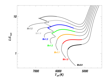
Figure 2.— HR diagram for models with $M=0.9-1.5$M_⊙ at solar metallicity. The thick colored lines show the range over which the three highest frequency avoided crossings were tracked.

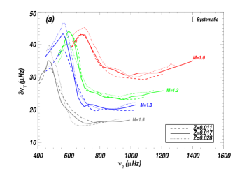
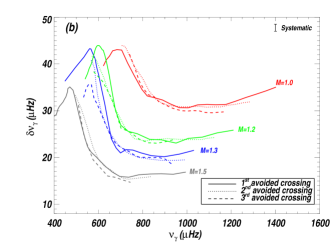
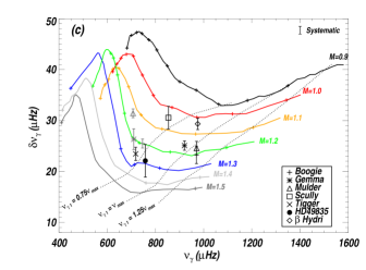
Figure 3.— (a): $\delta\nu_{\gamma}$ as a function of the $\gamma$-mode frequency for $\nu_{\gamma 1}$ and for $1.0M_{\odot}$ (red lines), $1.2M_{\odot}$ (green lines) and $1.3M_{\odot}$ (blue lines). Dashed, solid and dotted lines are for three metallicities Z.(b): $\delta\nu_{\gamma}$ as a function of $\nu_{\gamma 1}$ (solid lines), $\nu_{\gamma 2}$ (dotted lines) and $\nu_{\gamma 3}$ (dashed lines) at $Z=0.017$. (c): $\delta\nu_{\gamma}$ as a function of $\nu_{\gamma 1}$ for stellar masses $M_{\odot}=0.9$ to $M_{\odot}=1.5$, at $Z=0.017$. Crosses are spaced by $150$ Myr. Symbols correspond to the seven analyzed stars. Whenever reliable, fit values for the second measured avoided crossing are shown (gray symbols). Doted lines indicate when $\nu_{\gamma 1}=0.75\nu_{\rm max}$, $\nu_{\gamma 1}=\nu_{\rm max}$ and $\nu_{\gamma 1}=1.25\nu_{\rm max}$. They indicate the best region to observe the first avoided crossing.

5. Application to observed frequencies

We have applied the approach described above to the seven subgiants listed in Table 1. We use the published frequencies, which were measured either by ground-based spectroscopy, or from space by the CoRoT or Kepler missions.

Figure 3c shows the results. The symbols show the results of applying our method to the seven subgiants. The colored tracks are from the analysis of theoretical models discussed above, for a wide range of masses and a single metallicity, and only for the highest-frequency avoided crossing (the $\gamma_{1}$ mode). Crosses along each curve are spaced by 150 Myrs. We see that the $\gamma$-mode frequencies may vary by several hundreds of $\mu$Hz within this time scale while the precision of measure of these frequencies is only of few $\mu$Hz. Thus $\gamma$-mode frequencies provide a stringent constraint on stellar age.

We note that any potential deviation between the tracks of different metallicity (Figure 3a) and for different avoided crossings (Figure 3b) are within the uncertainties with which we can measure $\delta\nu_{\gamma}$. We can therefore superimpose results from more than one avoided crossing per star on the same diagram (Figure 3c). The quality of the data allowed us to extract accurately two avoided crossing in three Kepler stars (Mulder, Boogie and Gemma).

An example of a fit is shown in Figure 4 for Mulder. Despite its simplicity, the linear system of Eq. 2 can be useful to predict the position of previously unidentified mixed modes. Indeed, our method predicts an extra $\ell=1$ mixed mode, hardly seen on the power spectrum because it lies close to an $\ell=2$ mode (see Bedding 2011b for another example). This demonstrates that our method would allow us to identify $\ell=1$ mixed modes in complicated power spectra.

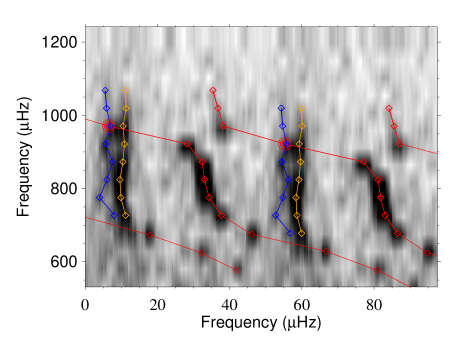
Figure 4.— Replicated échelle diagram (Bedding, 2011b) for Mulder Kepler target). Two avoided crossings are visible. The greyscale shows the observed power spectrum and open symbols show the frequencies reported by Campante et al. (2011). The model predicts an extra mixed mode (circles), not found by Campante et al. (2011) because it lies on an $\ell=2$ mode.

The results of the fit are given in Table 1. The first three columns give the identification number, the name and the observed $\nu_{\rm max}$ of each star. Columns 4–7 give the fitted values of $\nu_{\gamma}$ and $\delta\nu_{\gamma}$ for the avoided crossings. The last two columns give our inferred stellar mass, and the published mass found using conventional asteroseismic analysis. For the stars with published masses, our results agree well. However, in the case of HD 49835, the precision on the determination of $\delta\nu_{\gamma}$ is low (and so for the mass) because the avoided crossing occurs right at the lower boundary of the observed modes, with only one $\ell=1$ mode below $\nu_{\gamma_{1}}$.

The uncertainties on our mass estimates were obtained by linear interpolation between the tracks of different masses (cf. Figure 3c). As already noticed by Deheuvels & Michel (2011) mass and coupling are inversely proportional. Thus, uncertainties increase with mass because high-mass tracks are closer together than low-mass tracks. In the best cases, the total uncertainty (quadratic sum of the uncertainty of the measurement and of the systematic error) is a few percent, and in other cases it may be as large as $10\%$.

The results presented here are based on observed $\ell=1$ mixed modes. However, the mean large separation computed from the $\ell=0$ frequencies provides an independent way to measure stellar masses. Thus, the global accuracy, can be increased by using inferred masses from both the coupling strength and the mean large separation.

With observational data, not all the mixed modes can be seen because the mode envelope has a limited width. In order to indicate this in Figure 3c, the upward-sloping curves show where $\nu_{\gamma_{1}}=0.75\nu_{\rm max}$, $\nu_{\gamma_{1}}=\nu_{\rm max}$ and $\nu_{\gamma_{1}}=1.25\nu_{\rm max}$. Thus, these curves show the most likely region in which to observe the first avoided crossing. The most likely region to observe the second and third avoided crossings can be obtained by shifting these lines towards lower frequencies by $\approx 200\mu$Hz and $\approx 400\mu$Hz, respectively.

Table 1Measured mixed modes properties (minimal separation $\delta\nu_{\gamma}$ and $\gamma$-mode frequency, $\nu_{\gamma}$) and inferred mass $M$ (followed by its uncertainty and systematic error). For comparison, M_lit lists published masses derived by traditional seismic model fitting.

Id. Number	Nickname	$\nu_{\rm max}$ ($\mu$Hz)	$\nu_{\gamma_{1}}$ ($\mu$Hz)	$\delta\nu_{\gamma_{1}}$ ($\mu$Hz)	$\nu_{\gamma_{2}}$ ($\mu$Hz)	$\delta\nu_{\gamma_{2}}$ ($\mu$Hz)	M (M⊙)	Mlit (M⊙)
KIC 10273246	Mulder	$842$	$970.7\pm 3.2$	$24.6\pm 1.4$	$707.3\pm 1.2$	$31.4\pm 0.9$	$1.16\pm 0.03$ $(\pm 0.04)$
KIC 10920273	Scully	$974$	$854.1\pm 2.6$	$30.6\pm 2.3$			$1.04\pm 0.04$ $(\pm 0.04)$
KIC 11234888	Tigger	$675$	$718.4\pm 5.6$	$23.5\pm 1.3$			$1.27\pm 0.03$ $(\pm 0.10)$	$1.33\pm 0.26$
KIC 11395018	Boogie	$830$	$970.2\pm 10.6$	$23.3\pm 1.7$	$747.7\pm 0.6$	$25.6\pm 0.9$	$1.21\pm 0.06$ $(\pm 0.04)$	$1.25\pm 0.24$
KIC 11026764	Gemma	$857$	$920.7\pm 3.1$	$25.1\pm 1.0$	$710.2\pm 5.3$	$26.3\pm 2.1$	$1.17\pm 0.03$ $(\pm 0.05)$	$\simeq 1.13$ or $1.23$
HD 49835		$1013$	$758.3\pm 3.2$	$22.1\pm 3.2$			$1.30\pm 0.11$ $(\pm 0.06)$	$1.25\pm 0.05$
$\beta$ Hydri		$960$	$975.5\pm 1.6$	$29.3\pm 1.2$			$1.02\pm 0.06$ $(\pm 0.04)$	$1.08\pm 0.03$

Theoretically, the coupling strength should depend on the extent of the evanescent zone between the $g$-mode cavity in the core and the $p$-mode cavity of the envelope. Thus, it would be interesting to understand the exact nature of this relation, and why the minimal separation $\delta\nu_{\gamma}$ seems to depend strongly on stellar mass whereas it is the same for all avoided crossings and for a given star.

In this Letter, the effects of varying the mixing length parameter and the initial helium abundance have not been tested. They are known to be correlated to stellar mass and deserve further investigation.

References

- Aizenman et al. (1977) Aizenman, M., Smeyers, P., & Weigert, A. 1977, A&A, 58, 41
- Bedding (2011a) Bedding, T. R. 2011a, in Canary Islands Winter School of Astrophysics, Vol. XXII, Asteroseismology, ed. P. L. Pallé (Cambridge University Press), in press (arXiv:1107.1723)
- Bedding (2011b) Bedding, T. R. 2011b, in The 61st Fujihara seminar: Progress in solar/stellar physics with helio- and asteroseismology, ed. H. Shibahashi (ASP Conf. Ser.), in press (arXiv:1109.5768)
- Bedding et al. (2007) Bedding, T. R., Kjeldsen, H., Arentoft, T., et al. 2007, ApJ, 663, 1315
- Brandão et al. (2011) Brandão, I. M., et al. 2011, A&A, 527, A37
- Campante et al. (2011) Campante, T. L., et al. 2011, A&A, 534, A6
- Carrier et al. (2005) Carrier, F., Eggenberger, P., & Bouchy, F. 2005, A&A, 434, 1085
- Christensen-Dalsgaard (2008) Christensen-Dalsgaard, J. 2008, Ap&SS, 316, 13
- Christensen-Dalsgaard (2011) —. 2011, in the 61st Fujihara Seminar: Progress in solar/stellar physics with helio- and asteroseismology. ed. H. Shibahashi, ASP Conf. Ser, ArXiv:1110.5012
- Christensen-Dalsgaard et al. (1995) Christensen-Dalsgaard, J., Bedding, T. R., & Kjeldsen, H. 1995, ApJ, 443, L29
- Deheuvels & Michel (2010a) Deheuvels, S., & Michel, E. 2010a, Ap&SS, 328, 259
- Deheuvels & Michel (2010b) —. 2010b, Astron. Nachr., 331, 929
- Deheuvels & Michel (2011) —. 2011, A&A, 535, A91
- Deheuvels et al. (2010) Deheuvels, S., et al. 2010, A&A, 515, A87
- di Mauro et al. (2011) di Mauro, M. P., et al. 2011, MNRAS, 415, 3783
- Dupret et al. (2009) Dupret, M.-A., et al. 2009, A&A, 506, 57
- Eggleton et al. (1973) Eggleton, P. P., Faulkner, J., & Flannery, B. P. 1973, A&A, 23, 325
- Gough (1986) Gough, D. O. 1986, in Hydrodynamic and Magnetodynamic Problems in the Sun and Stars, ed. Y. Osaki (Tokyo: Uni. of Tokyo Press), 117
- Grevesse & Noels (1993) Grevesse, N., & Noels, A. 1993, Cambridge University press, 15
- Kjeldsen et al. (1995) Kjeldsen, H., Bedding, T. R., Viskum, M., & Frandsen, S. 1995, AJ, 109, 1313
- Kjeldsen et al. (2003) Kjeldsen, H., et al. 2003, AJ, 126, 1483
- Kurucz (1991) Kurucz, R. L. 1991, in NATO ASIC Proc. 341: Stellar Atmospheres - Beyond Classical Models, ed. L. Crivellari, I. Hubeny, & D. G. Hummer, 441
- Mathur et al. (2010) Mathur, S., et al. 2010, A&A, 511, A46
- Mathur et al. (2011) —. 2011, ApJ, 733, 95
- Metcalfe et al. (2010) Metcalfe, T. S., et al. 2010, ApJ, 723, 1583
- Osaki (1975) Osaki, J. 1975, PASJ, 27, 237
- Rogers & Iglesias (1995) Rogers, F. J., & Iglesias, C. A. 1995, in Astronomical Society of the Pacific Conference Series, Vol. 78, Astrophysical Applications of Powerful New Databases, ed. S. J. Adelman & W. L. Wiese, 31
- Stello (2011) Stello, D. 2011, in the 61st Fujihara Seminar: Progress in solar/stellar physics with helio- and asteroseismology. ed. H. Shibahashi, ASP Conf. Ser, ArXiv:1107.1311
- Stello et al. (2009) Stello, D., et al. 2009, ApJ, 700, 1589
- Tassoul (1980) Tassoul, M. 1980, ApJS, 43, 469
- Vandakurov (1967) Vandakurov, Y. V. 1967, AZh, 44, 786