Numerical Calculation of Convection with Reduced Speed of Sound Technique

Abstract

Context. The anelastic approximation is often adopted in numerical calculation with low Mach number, such as stellar internal convection. This approximation requires frequent global communication, because of an elliptic partial differential equation. Frequent global communication is negative factor for the parallel computing with a large number of CPUs.

Aims. The main purpose of this paper is to test the validity of a method that artificially reduces the speed of sound for the compressible fluid equations in the context of stellar internal convection. The reduction of speed of sound allows for larger time steps in spite of low Mach number, while the numerical scheme remains fully explicit and the mathematical system is hyperbolic and thus does not require frequent global communication.

Methods. Two and three dimensional compressible hydrodynamic equations are solved numerically. Some statistical quantities of solutions computed with different effective Mach numbers (due to reduction of speed of sound) are compared to test the validity of our approach.

Results. Numerical simulations with artificially reduced speed of sound are a valid approach as long as the effective Mach number (based on the reduced speed of sound) remains less than 0.7.

1 Introduction

Turbulent thermal convection in the solar convection zone plays a key role for the maintenance of large scale flows (differential rotation, meridional flow) and solar magnetic activity. The angular momentum transport of convection maintains the global mean flows. Global flows relate to the generation of global magnetic field, i.e. the solar dynamo. Differential rotation bends the pre-existing poloidal field and generates the strong toroidal field ($\Omega$ effect) and mean meridional flow transports the magnetic flux equatorward at the base of the convection zone (Choudhuri et al., 1995; Dikpati & Charbonneau, 1999). The internal structures of the solar differential rotation and the meridional flow are revealed by the helioseismology (see review by Thompson et al., 2003). Some mean field studies have reproduced these global flow (Kichatinov & Rüdiger, 1993; Küker & Stix, 2001; Rempel, 2005; Hotta & Yokoyama, 2011). These studies, however, used some kinds of parameterization of the turbulent convection, i.e. turbulent viscosity and turbulent angular momentum transport. Thus, a self-consistent thorough understanding of global structure requires the detailed investigation of the turbulent thermal convection. Turbulent convection is important also in the magnetic field itself. The strength of the next solar maximum in the prediction by the mean field model significantly depends on the turbulent diffusivity (Dikpati & Gilman, 2006; Choudhuri et al., 2007; Yeates et al., 2008). In addition, the turbulent diffusion has an important role in the parity of solar global field, the strength of polar field and so on (Hotta & Yokoyama, 2010a, b).

There are already numerous LES numerical simulations on the solar and stellar convection (Gilman, 1977; Gilman & Miller, 1981; Glatzmaier, 1984; Miesch et al., 2000, 2006; Brown et al., 2008) and these magnetic fields (Gilman & Miller, 1981; Brun et al., 2004; Brown et al., 2010, 2011). In these studies the anelastic approximation is adopted to avoid the difficulty which is caused by the high speed of sound. At the base of convection zone the speed of sound is about $200\ \mathrm{km\ s^{-1}}$. In contrast the speed of convection is thought to be 50 $\mathrm{m\ s^{-1}}$ (Stix, 2004), so the time step must be shortened due to the CFL condition in explicit fully compressible method, even when we are interested in phenomena related to convection. In the anelastic approximation, equation of continuity is treated as

$$\nabla\cdot(\rho_{0}{\bf v})=0,$$ (1)

where $\rho_{0}$ is stratified background density and ${\bf v}$ denotes the velocity. The anelastic approximation assumes that the speed of sound is essentially infinite, resulting in an instantaneous adjustment of pressure to flow changes. This is achieved by solving an elliptic equation for the pressure, which filters out the propagation of sound waves. As a result the time step is only limited by the much lower flow velocity. However, due to the existence of an elliptic the anelastic approximation has a weak point. The numerical calculation in parallel computing requires the frequent global communication. At the present time the efficiency of scaling in parallel computing is saturated with about 2000-3000 CPUs in solar global simulation with pseudo-spectral method (M. Miesch private communication). More and more resolution, however, is thought to be needed to understand the precise mechanism of the angular momentum and energy transport by the turbulent convection and the behavior of magnetic field especially in thin magnetic flux tube.

In this paper, we test the validity of a different approach to circumvent the severe numerical time step constraints in low Mach number flows. We use a method in which the speed of sound is reduced artificially by transforming the equation of continuity to (see, e.g., Rempel, 2005)

$$\frac{\partial\rho}{\partial t}=-\frac{1}{\xi^{2}}\nabla\cdot(\rho{\bf v}),$$ (2)

where $t$ denotes the time. Using this equation, the effective speed of sound becomes $\xi$ times smaller, but otherwise the dispersion relationship for sound wave remains unchanged (wave speed is dropped for all wavelength equally). Since this technique does not change the hyperbolic character of the underlying equations, the numerical treatment can remain fully explicit and thus does not require global communication in parallel computing. We will call the technique in the following the Reduced Speed of Sound Technique (RSST). This technique has been used previously by Rempel (2005, 2006) in mean field models for solar differential rotation and non-kinematic dynamos, which essentially solve the full set of time dependent axisymmetric MHD equations. Those solutions were however restricted to the relaxation toward a stationary state or very slowly varying problems on the time scale of the solar cycle. Here we will apply this approach to thermal convection, where the intrinsic time scales are substantially shorter. To this end we study two and three dimensional convection, in particular the latter will be non-stationary and turbulent.

The detailed setting of test calculation is given in Section 2. The results of our calculations are given in Section 3. We summarize our paper and give discussion of the RSST in Section 4.

2 Model

2.1 Equations

The two or three dimensional equation of continuity, equation of motion, equation of energy, equation of state, are solved in Cartesian coordinate $(x,z)$ or $(x,y,z)$, where $x$ and $y$ denote the horizontal direction and $z$ denotes the vertical direction. The basic assumptions underlying this study are as follows.

1. Time independent hydrostatic reference state.

2. The perturbations caused by thermal convection are small, i.e. $\rho_{1}\ll\rho_{0}$ and $p_{1}\ll p_{0}$, Here $\rho_{0}$ and $p_{0}$ denote the reference state values, whereas $\rho_{1}$ and $p_{1}$ are the fluctuations of density and pressure, respectively. Thus a linearized equation of state is used as eq. (6)

3. The profile of the reference entropy $s_{0}(z)$ is a steady state solution of the thermal diffusion equation $\nabla\cdot(K\rho_{0}T_{0}\nabla s_{0})=0$ with constant $K$.

The formulations are almost same as Fan et al. (2003). Equations are expressed as,

$$\frac{\partial\rho_{1}}{\partial t}=-\frac{1}{\xi^{2}}\nabla\cdot(\rho_{0}{\bf v}),$$ (3)

$$\frac{\partial{\bf v}}{\partial t}=-({\bf v}\cdot\nabla){\bf v}-\frac{\nabla p_{1}}{\rho_{0}}-\frac{\rho_{1}}{\rho_{0}}g{\bf e_{z}}+\frac{1}{\rho_{0}}\nabla\cdot{\bf\Pi},$$ (4)

$$\frac{\partial s_{1}}{\partial t}=-({\bf v}\cdot\nabla)(s_{0}+s_{1})+\frac{1}{\rho_{0}T_{0}}\nabla\cdot(K\rho_{0}T_{0}\nabla s_{1})$$

$$+\frac{\gamma-1}{p_{0}}({\bf\Pi}\cdot\nabla)\cdot{\bf v},$$ (5)

$$p_{1}=p_{0}\left(\gamma\frac{\rho_{1}}{\rho_{0}}+s_{1}\right),$$ (6)

where $T_{0}(z)$, and $s_{0}(z)$ denote reference temperature, and entropy, respectively and ${\bf e_{z}}$ denotes the unit vector along the $z$-direction. $\gamma$ is the ratio of specific heats, with the value for an ideal gas being $\gamma=5/3$. $s_{1}$ denotes the fluctuation of entropy from reference atmosphere. Note that the entropy is normalized by specific heat capacity at constant volume $c_{\mathrm{v}}$. The quantity $g$ is the gravitational acceleration, which is assumed to be constant. The quantity ${\bf\Pi}$ denotes the viscous stress tensor,

$$\Pi_{ij}=\rho_{0}\nu\left[\frac{\partial v_{i}}{\partial x_{j}}+\frac{\partial v_{j}}{\partial x_{i}}-\frac{2}{3}(\nabla\cdot{\bf v})\delta_{ij}\right],$$ (7)

and $\nu$ and $K$ denote the viscosity and thermal diffusivity, respectively. $\nu$ and $K$ are assumed to be constant throughout the simulation domain. We assume for the reference atmosphere a weakly superadiabatically stratified polytrope:

$$\rho_{0}(z)=\rho_{r}\left[1-\frac{z}{(m+1)H_{r}}\right]^{m},$$ (8)

$$p_{0}(z)=p_{r}\left[1-\frac{z}{(m+1)H_{r}}\right]^{m+1},$$ (9)

$$T_{0}(z)=T_{r}\left[1-\frac{z}{(m+1)H_{r}}\right],$$ (10)

$$H_{p}(z)=\frac{p_{0}}{\rho_{0}g},$$ (11)

$$\frac{ds_{0}}{dz}=-\frac{\gamma\delta(z)}{H_{p}(z)},$$ (12)

$$\delta(z)=\delta_{r}\frac{\rho_{r}}{\rho_{0}(z)},$$ (13)

where $\rho_{\mathrm{r}}$, $p_{\mathrm{r}}$, $T_{\mathrm{r}}$, $H_{\mathrm{r}}$, and $\delta_{\mathrm{r}}$ denote the values of $\rho_{0}$, $p_{0}$, $T_{0}$, $H_{0}$ (the pressure scale height) and $\delta$ (the non-dimensional superadiabaticity) at the bottom boundary $z=0$. Since $|\delta|\ll 1$, the value $m$ is nearly equal to the adiabatic value, meaning $m=1/(\gamma-1)$. The strength of the diffusive parameter $\nu$ and $K$ is expressed with following non-dimensional parameters: the Reynolds number $\mathrm{Re}\equiv v_{\mathrm{c}}H_{\mathrm{r}}/\nu$, and the Prandtl number $\mathrm{Pr}\equiv\nu/K$, where the velocity unit $v_{\mathrm{c}}\equiv(8\delta_{\mathrm{r}}gH_{\mathrm{r}})^{1/2}$. Note that in this paper the unit of time is $H_{\mathrm{r}}/v_{\mathrm{c}}$. In all calculations, we set $\mathrm{Pr}=1$.

2.2 Boundary Conditions and Numerical Method

We solve equations (3)-(6) numerically. At the horizontal boundaries ($x=0,\ L_{x}$ and $y=0,\ L_{y}$), periodic boundary conditions are adopted for all variables. At the top and the bottom boundaries impenetrative and stress free boundary conditions are adopted for the velocities and the entropy is fixed:

$$v_{z}=0,$$ (14)

$$\frac{\partial v_{x}}{\partial z}=0,$$ (15)

$$\frac{\partial v_{y}}{\partial z}=0,$$ (16)

$$s_{1}=0.$$ (17)

At both top and bottom boundaries ($z=0$ and $z=L_{z}$), we set $p_{1}$ in the ghost cells such that the right hand side of the z-component of eq. (4) is zero at the boundary (which is between ghost cells and domain cells), where the ghost cells are the cells beyond the physical boundary.

We adopt the fourth-order space-centered difference for each derivative. The first spatial derivatives of quantity $q$ is given by

$$\left(\frac{\partial q}{\partial x}\right)_{i}=\frac{1}{12\Delta x}(-q_{i+2}+8q_{i+1}-8q_{i-1}+q_{i-2}),$$ (18)

where $i$ denotes the index of the grid position along a particular spatial direction. The numerical solution of the system is advanced in time with an explicit fourth-order Runge-Kutta scheme. The system of partial equations can be written as

$$\frac{\partial{\bf U}}{\partial t}={\bf R(U)}$$ (19)

${\bf U}_{n+1}$, which is the value at $t_{n+1}=(n+1)\Delta t$ is calculated in four steps:

$${\bf U}_{n+\frac{1}{4}}={\bf U}_{n}+\frac{\Delta t}{4}{\bf R}({\bf U}_{n}),$$ (20)

$${\bf U}_{n+\frac{1}{3}}={\bf U}_{n}+\frac{\Delta t}{3}{\bf R}({\bf U}_{n+\frac{1}{4}}),$$ (21)

$${\bf U}_{n+\frac{1}{2}}={\bf U}_{n}+\frac{\Delta t}{2}{\bf R}({\bf U}_{n+\frac{1}{3}}),$$ (22)

$${\bf U}_{n+1}={\bf U}_{n}+\Delta t{\bf R}({\bf U}_{n+\frac{1}{2}}).$$ (23)

The maximum allowed time step, $\Delta t_{\mathrm{max}}$, is determined by the CFL criterion. When both advection and diffusion terms are included in calculation, the time step reads,

$$\Delta t_{\mathrm{max}}=\min(\Delta t_{\mathrm{ad}},\Delta t_{\mathrm{v}}).$$ (24)

Here

$$\Delta t_{\mathrm{ad}}=c_{\mathrm{ad}}\frac{\min(\Delta x,\Delta y,\Delta z)}{c_{\mathrm{tot}}}.$$ (25)

$c_{\mathrm{tot}}$ is the total wave speed:

$$c_{\mathrm{tot}}=|v|+c^{\prime}_{\mathrm{s}},$$ (26)

where the effective speed of sound is expressed as:

$$c^{\prime}_{\mathrm{s}}=\frac{1}{\xi}\sqrt{\gamma\frac{p_{0}}{\rho_{0}}}.$$ (27)

The time step determined by diffusion term is

$$\Delta t_{\mathrm{v}}=c_{\mathrm{v}}\frac{\min(\Delta x^{2},\Delta y^{2},\Delta z^{2})}{\max(K,\nu)}.$$ (28)

$c_{\mathrm{ad}}$ and $c_{\mathrm{v}}$ are safety factors of order unity.

Using $\delta_{\mathrm{r}}=1\times 10^{-4}$, the original speed of sound is about 35$v_{\mathrm{c}}$ at the bottom and 12$v_{\mathrm{c}}$ at the top boundary, respectively. In all calculation $\Delta x\sim 2.3\times 10^{-2}H_{\mathrm{r}}$. Thus if we use $c_{\mathrm{ad}}=1$ and $c_{\mathrm{v}}=1$, $\Delta t_{\mathrm{ad}}=6.4\times 10^{-4}\ H_{\mathrm{r}}/v_{\mathrm{c}}$ and $\Delta t_{\mathrm{v}}=1.5\times 10^{-1}\ H_{\mathrm{r}}/v_{\mathrm{c}}$. For all the $\xi$ values considered in this paper the time step remains restricted by the (reduced) speed of sound, thus the calculation has about $\xi$ times better efficiency with the RSST.

3 Result

3.1 Two Dimensional Study

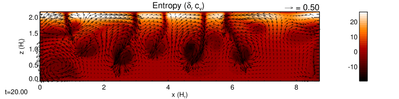
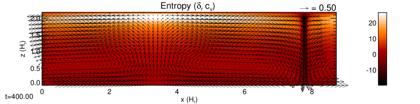
Figure 1: Time-development of entropy in a two-dimensional calculation with parameters of case 1. (Top panel) $t=20$. (Bottom panel) $t=400$.

Four two-dimensional calculations with the RSST and one calculation without approximation are carried out (case 1-5). The values of free-parameters are given in Table 1. The superadiabaticity ($\delta$) is $1\times 10^{-6}$ at the bottom and about $2\times 10^{-5}$ at the top boundary. It is almost the same superadiabaticity value as the base of solar convection zone. Fig. 1 shows the time-development of entropy. In the beginning the non-linear time dependent convection developed (top panel), which transitions to a steady state at later times (bottom panel). In the steady state, we compare the RMS velocity with different $\xi$. The RMS velocity is defined as:

$$v_{\mathrm{RMS}}=\sqrt{\frac{1}{L_{x}L_{y}}\int_{0}^{L_{x}}\int_{0}^{L_{y}}v^{2}dxdy}.$$ (29)

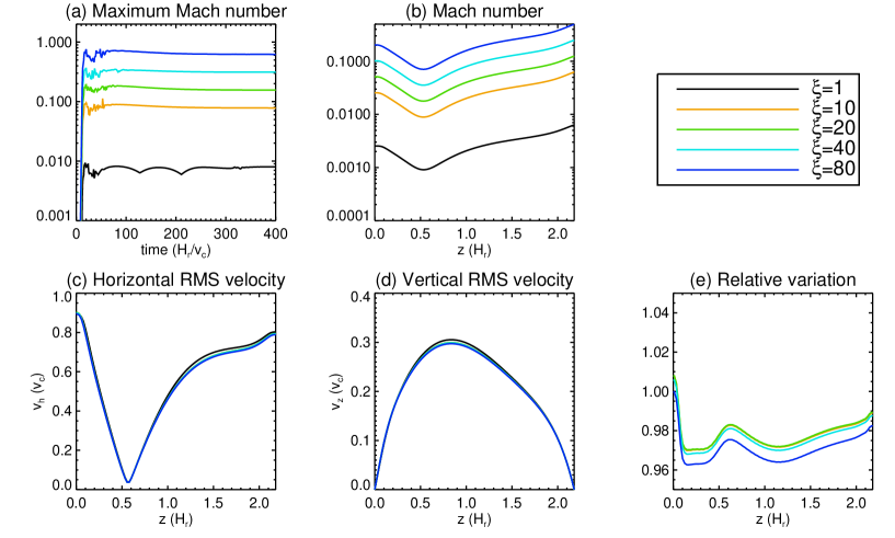
Figure 2: Some quantities in two dimensional calculation.(a) Maximum Mach number of each time step. (b) Distribution of Mach number estimated with the RMS velocity. (c) Distribution of horizontal RMS velocity $v_{\mathrm{h}}$. (d) Distribution of vertical RMS velocity. (e) Ratio between the RMS velocities with each $\xi$ and $\xi=1$.

Fig. 2 shows our results with the value of $\xi$ being from 1 to 80. The effective Mach number is defined as $M_{\mathrm{A}}=v_{\mathrm{RMS}}/c^{\prime}_{\mathrm{s}}$. If we have larger $\xi$ value than 80, we cannot obtain stationary state, since there are some shock generated by supersonic convection. The discussion of unsteady convection is given in the next session of three-dimensional calculations. Even though the Mach number reaches 0.6 using $\xi=80$ (panel a), the horizontal and vertical RMS velocity is almost same as those calculated with $\xi=1$ (without RSST). The ratio between the RMS velocities with each $\xi$ and $\xi=1$ are shown in Fig. 2e. The deviation is always a few percent. This result is not surprising since in the stationary state the equation of continuity becomes

$$0=\frac{1}{\xi^{2}}\nabla\cdot(\rho_{0}{\bf v}),$$ (30)

whose solution must not depend on the value of $\xi$. We note that the cell size is to some degree affected by the aspect ratio of the domain. This does not affect our conclusions since this influence is the same for all values of $\xi$ considered. To confirm the robustness of our conclusions we repeated this experiment with a wider domain ($26.16H_{r}\times 2.18H_{r}$ instead of $8.72H_{r}\times 2.18H_{r}$) in which we find 4 steady convection cells with about $10\%$ different RMS velocities. Also here we find a dependence on $\xi$ similar to that shown in Fig. 2, i.e. the solutions show differences of only a few percent as long as $\xi<80$. In this section we confirm that the RSST is valid for the two-dimensional stationary convection when the effective Mach number is less than 1, i.e. $\xi<80$ with $\delta_{\mathrm{r}}=1\times 10^{-6}$. If we use $\delta_{\mathrm{r}}=1\times 10^{-4}$ (result is not shown), the criterion becomes $\xi<8$ in two dimensional calculation.

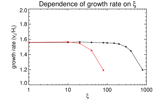
Figure 3: Behavior in linear phase. Dependence of growth rate on $\xi$ is shown. Black and red lines show the results with $\delta_{\mathrm{r}}=1\times 10^{-6}$ and $1\times 10^{-4}$, respectively.

As a next step we investigate the dependence of the linear growth rate on $\xi$ during the initial (time dependent) relaxation phase toward the final stationary state. Fig. 3 shows the linear growth of maximum perturbation density $\rho_{1}$ with different $\xi$. Black and red lines show the results with $\delta_{\mathrm{r}}=1\times 10^{-6}$ and $\delta_{\mathrm{r}}=1\times 10^{-4}$, respectively. These calculation parameters are not given in Table 1. In the calculation with $\delta=1\times 10^{-6}$ the growth rate decreases for values of $\xi>300$, whereas it occurs $\xi>30$ in the calculation with $\delta_{\mathrm{r}}=1\times 10^{-4}$. The reason can be explained as follows: In the convective instability, upflow (downflow) generates positive (negative) entropy perturbation and then negative (positive) density perturbation is generated by the sound wave. If the speed of sound is fairly slow, the generation mechanism of density perturbation is ineffective. In the calculation with $\delta_{\mathrm{r}}=1\times 10^{-6}$ ($\delta_{\mathrm{r}}=1\times 10^{-4}$), the growth rate with $\xi=200$ ($\xi=20$), however, is almost same as that with $\xi=1$, even though flow with $\xi=200$ ($\xi=20$) is expected to be the Mach number $Ma=1.3$, i.e. supersonic convection flow in the saturated state.

3.2 Three Dimensional Study

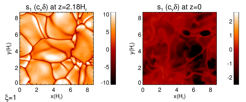
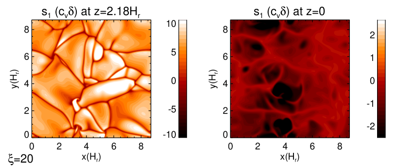
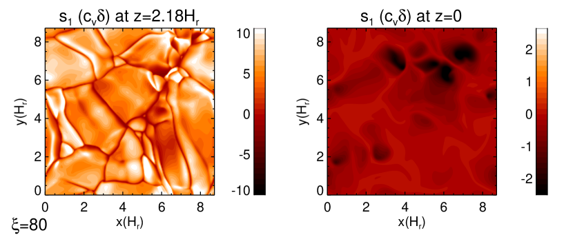
Figure 4: Snapshots of entropy of the three-dimensional convection. Top, middle, and bottom panels correspond to $\xi=1$, 10 and 80 respectively. Left (right) panels show entropy at top (bottom) boundary. (Animation is provided, and the difference between $\xi=1$ and $80$ is best visible in the animation of Fig. 4 that is provided with the online version.)

In this section, we investigate the validity of the RSST with three-dimensional unsteady thermal convections (case 6-13). The value of superadiabaticity at the bottom boundary is $1\times 10^{-4}$ and at the top $2\times 10^{-3}$. Although this value is relatively large compared with solar value, the expected speed of convection is much smaller than speed of sound, so it is small enough to investigate the validity of the RSST. Entropy of three-dimensional convections with $\xi=1$, 20, and 80 at $t=100H_{\mathrm{r}}/v_{\mathrm{c}}$ are shown in Fig. 4. The convection is completely unsteady and turbulent (animation is provided). The appearance of convection with $\xi=20$ is almost same as that with $\xi=1$. This will be verified below by the Fourier transformation and auto-detection technique. On the other hand, the appearance of convection with $\xi=80$ (bottom panel) is completely different from the others. This difference is best visible in the animation of Fig. 4 that is provided with the online version.

RMS velocities with different $\xi$ are estimated as average of values between $t=100$ to $200H_{\mathrm{r}}/v_{\mathrm{c}}$ (Fig. 5: panel b and c). Without the RSST, i.e. $\xi=1$ and using $\delta_{\mathrm{r}}=1\times 10^{-4}$, the Mach number is $1\times 10^{-2}$ at the bottom and $4\times 10^{-2}$ at the top boundary. The RMS velocities at $\xi=40$ and 80 differ from those at the $\xi=1$ by less than $15\ \%$ and $30\ \%$, respectively. When we adopt $\xi=40$ and 80, the Mach number estimated by RMS velocity exceeds unity (Fig. 5: panel a), i.e. supersonic convection. This supersonic downflow frequently generates shocks and positive entropy perturbation, thus downflow is slowed. This is the reason why the RMS velocities with large $\xi(=40,80)$ are small. When $\xi=5$, 10, 15, and 20, however, the RMS velocities show good agreement with that with $\xi=1$. RMS power density of pressure, buoyancy and inertia are estimated (Fig. 5). This results shows almost the same tendency as the result of RMS velocities. Power profiles $\xi=5$, 10, 15, 20 show agreement and those with $\xi=40$, 80 shows discrepancy with those with $\xi=1$. These results show that the RSST is valid technique with at least $\xi=20$ with which the Mach number is around $0.7$. Note that the convection pattern in our 2D and 3D cases differs substantially. As a consequence, also the $\xi$ values for which the validity of RSST breaks down are also different in 2D and 3D setups.

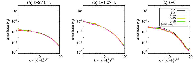
Figure 6: Comparison of horizontal velocity spectra with different $\xi$. (a) $z=2.18H_{r}$ (b) $z=1.09H_{r}$ (c) $z=0$. Velocities are averaged in time between $t=100$ and $200H_{\mathrm{r}}/v_{\mathrm{c}}$

In Fig. 6 we compare averaged spectral amplitudes for different values of $\xi$. There is no significant difference between the spectral amplitudes for different values of $\xi$ in the range from 1 to 20.

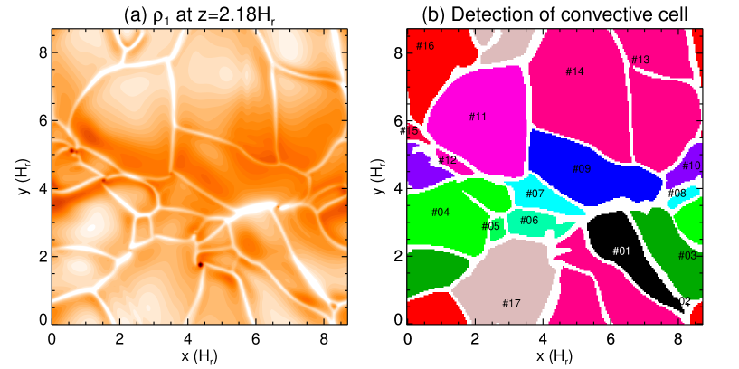
Figure 7: Detection of convective cell. (a) Original contour of density perturbation at $z=2.18H_{r}$ (b) Distribution of detected convection cell. Color and label (#n) show each convective cell.

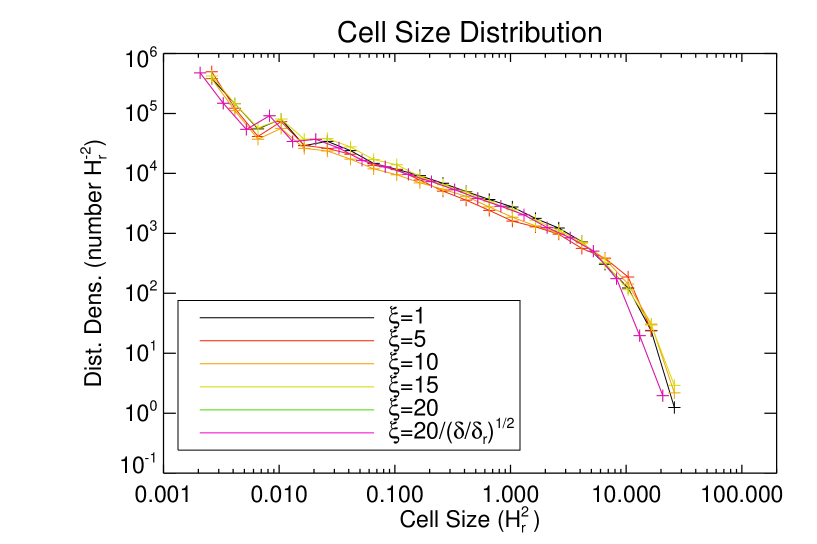
Figure 8: Distribution of convective cell size with different $\xi$ is shown. The cell size distribution is averaged in time between $t=100$ and $200H_{\mathrm{r}}/v_{\mathrm{c}}$.

We investigate the distribution of cell size at the top boundary. This value is significantly related to the turbulent diffusivity and transport of angular momentum or energy. The method to detect the cell is explained as follows. At the boundary of the cell i.e., the region of downflow, the perturbation of density is positive and has large value. When the density in a region exceeds a threshold, the region is regarded as boundary of convective cell. When a region is surrounded by one continuous boundary region, the region is defined as one convective cell. Fig. 7 shows the detected cells. Each color and each label (#n) correspond to each detected cell. We estimate size of all cells and compare the distribution of cell size with different $\xi$. The results are shown in Fig. 8. The cell size distribution follows a power law from about 0.01 to 10 $H_{\mathrm{r}}^{2}$ and there is no dependence on $\xi$ in the range from 1 to 20. Although using this type of technique size of cells is tend to be large with neglecting smaller cells, our conclusion is not wrong, since all the auto detections are affected equally.

With above two investigations, i.e. the Fourier analysis and study of cell detection, we can conclude that the statistical features are not influenced by the RSST as long as the effective Mach number (computed with the reduced speed of sound) does not exceed values of about 0.7, which corresponds to $\xi=20$ in our setup.

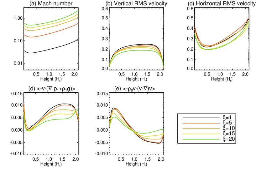
Figure 9: The results with $\delta_{\mathrm{r}}=1\times 10^{-3}$. The format is the same as Fig. 5

In order to confirm our criterion that the RSST is valid if the Mach number is smaller than 0.7, we conduct calculations with larger superadiabaticity, i.e. $\delta_{\mathrm{r}}=1\times 10^{-3}$ (Case 14-18). If our criterion is valid, required $\xi$ with larger superadiabaticity must decrease. The results are shown in Fig. 9. Using $\delta_{\mathrm{r}}=1\times 10^{-3}$, the calculations with $\xi=10$, $15$, and $20$ generate supersonic convection flow near the surface (Fig. 9a). It is clear that the results with $\xi=10$, $15$ and $20$ differ from that with $\xi=1$ and $5$. The calculation with $\xi=5$ shows flow whose Mach number is around 0.6. Thus our criterion is not violated even with different value of the superadiabaticity.

Due to our changed equation of continuity the primitive and conservative formulation of Eq. (3) to (5) are not equivalent anymore. For example, the equation of motion in conservative form is expressed as:

$$\frac{\partial}{\partial t}(\rho{\bf v})=-\nabla\cdot(\rho{\bf vv})+{\bf F},$$ (31)

where ${\bf F}$ denotes pressure gradient, gravity and Lorentz force. With some transformations we can obtain,

$${\bf v}\frac{\partial\rho}{\partial t}+\rho\frac{\partial{\bf v}}{\partial t}=-{\bf v}\nabla\cdot(\rho{\bf v})-\rho({\bf v}\cdot\nabla){\bf v}+{\bf F}$$ (32)

If equation of continuity is satisfied, i.e. ($\partial\rho/\partial t=-\nabla\cdot(\rho{\bf v})$), the primitive form is obtained as:

$$\rho\frac{\partial{\bf v}}{\partial t}=\rho({\bf v}\cdot\nabla){\bf v}+{\bf F}.$$ (33)

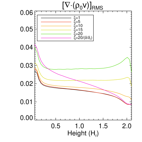
Figure 10: Dependence of $[\nabla\cdot(\rho_{0}{\bf v})]_{\mathrm{RMS}}$ on $\xi$. In case 13, the value of $\xi$ is 20 at the bottom and 4.5 at the top boundary.

However, using the RSST these two form are no longer equivalent. We used here the primitive formulation at the expense that energy and momentum are not strictly conserved; however, the consistency of our results for different values $\xi$ strongly indicates that this is not a serious problem for the setup we considered. Alternatively we could also implement our modified equation of continuity into a conservative formulation. This would ensure that density, momentum and energy are strictly conserved at the expense of a modified set of primitive equations. Fig. 10 shows the dependence of $[\nabla\cdot(\rho_{0}{\bf v})]_{\mathrm{RMS}}\ (=[\xi^{2}\partial\rho_{1}/\partial t]_{\mathrm{RMS}})$ on $\xi$. Using $\xi=5$, this term is almost same as that with $\xi=1$. Although the deviation becomes large as $\xi$ increases, it is not proportional to $\xi^{2}$.

In the previous discussion we kept $\xi$ constant in the entire computational domain. In the solar convection zone the Mach number varies however substantially with depth, from $\sim 1$ in the photosphere to $<10^{-7}$ at the base of the convection zone, the speed of sound itself varies from about $7\ \mathrm{km\ s^{-1}}$ in the photosphere to $200\ \mathrm{km\ s^{-1}}$ at the base of the convection zone. A reduction of the speed of sound is therefore most important in the deep convection zone, but not in the near surface layers. This could be achieved with a depth dependent $\xi$. Even if we use conservative form as,

$$\frac{\partial\rho_{1}}{\partial t}=-\nabla\cdot\left(\frac{1}{\xi^{2}}\rho_{0}{\bf v}\right),$$ (34)

the result must not be same as the result without approximation in statistical steady state. When the value averaged in statistical steady state is expressed as $\langle a\rangle$, where $a$ is a physical value, the equation of continuity becomes

$$0=\nabla\cdot\left(\frac{1}{\xi^{2}}\rho_{0}\langle{\bf v}\rangle\right),$$ (35)

with inhomogeneous $\xi$. The solution of Eq. (35) is different from the solution of original equation of continuity in statistical steady state, i.e. $0=\nabla\cdot(\rho_{0}\langle{\bf v}\rangle)$. Thus, the statistical features such as RMS velocity are not reproduced with inhomogeneous $\xi$. If we use the non-conservative form of equation of motion as Eq. (2), this problem does not occur. Thus we investigate the nonuniformity of $\xi$ in case 13 using non-conservative form, i.e., eq. (3). In order to keep the Mach number uniform in all the height, we use $\xi=20/(\delta(z)/\delta_{r})^{1/2}$, i.e. $\xi=20$ at the bottom and $\xi=4.5$ at the top boundary. Note that the ratio of the speed of convection to the speed of sound is roughly estimated as $\sqrt{\delta}$. In this setting the value of $\sqrt{\delta}$ is $1\times 10^{-2}$ at the bottom and $4\times 10^{-2}$ at the top boundary. The same analysis as that for uniform $\xi$ is done (see Fig. 5, 6 and 10). There is no significant difference between $\xi=20/(\delta(z)/\delta_{r})^{1/2}$ and $\xi=1$. Although mass is not conserved locally with non-homogeneous $\xi$ using non-conservative form, horizontally averaged vertical mass flux is approximately zero in the statistically steady convection and the conservation total mass is not significantly broken. We conclude that an inhomogeneous $\xi$ is valid under the previously obtained condition, i.e. the Mach number is less than 0.7.

4 Summary and Discussion

In this paper we applied RSST (see Section 1) to two and three dimensional simulations of low Mach number thermal convection and confirmed the validity of this approach as long as the effective Mach number (computed with the reduced speed of sound) stays below 0.7 everywhere in the domain. The overall gain in computing efficiency that can be achieved depends therefore on the maximum Mach number that was present in the setup of the problem.

Since the Mach number is estimated to be $10^{-4}$ in the base of solar convection zone (Stix, 2004), several thousand times longer time step can be taken using the RSST. Therefore the RSST and parallel computing with large number of CPUs will make it possible to calculate large scale solar convection with high resolution in the near future.

Compared to the anelastic approximation there are three major advantages in RSST:

1. It can be easily implemented into any fully compressible code (regardless of numerical scheme or grid structure) since it only requires a minor change of the equation of continuity and leaves the hyperbolic structure of the equations unchanged.

2. Due to the explicit treatment it does not require any additional communication overhead, which makes it suitable for massive parallel computations.

3. The base of the convection zone and the surface of the sun where the anelastic approximation is broken can be connected, using space dependent $\xi$.

Overall we find that RSST is a very useful technique for studying low Mach number flows in stellar convection zones as it substantially alleviates stringent time step constraints without adding computational overhead.

Table 1: Parameters for numerical simulations. In case 13 the value of $\xi$ is 20 at the bottom and 4.5 at the top boudary.

Case	dimension	$L_{x}\times L_{y}\times L_{z}(H_{r})$	$N_{x}\times N_{y}\times N_{z}$	$\delta_{r}$	Re	$\xi$
1	2	$8.72\times 2.18$	$384\times 96$	$1\times 10^{-6}$	260	1
2	2	$8.72\times 2.18$	$384\times 96$	$1\times 10^{-6}$	260	10
3	2	$8.72\times 2.18$	$384\times 96$	$1\times 10^{-6}$	260	30
4	2	$8.72\times 2.18$	$384\times 96$	$1\times 10^{-6}$	260	50
5	2	$8.72\times 2.18$	$384\times 96$	$1\times 10^{-6}$	260	80
6	3	$8.72\times 8.72\times 2.18$	$384\times 384\times 96$	$1\times 10^{-4}$	300	1
7	3	$8.72\times 8.72\times 2.18$	$384\times 384\times 96$	$1\times 10^{-4}$	300	5
8	3	$8.72\times 8.72\times 2.18$	$384\times 384\times 96$	$1\times 10^{-4}$	300	10
9	3	$8.72\times 8.72\times 2.18$	$384\times 384\times 96$	$1\times 10^{-4}$	300	15
10	3	$8.72\times 8.72\times 2.18$	$384\times 384\times 96$	$1\times 10^{-4}$	300	20
11	3	$8.72\times 8.72\times 2.18$	$384\times 384\times 96$	$1\times 10^{-4}$	300	40
12	3	$8.72\times 8.72\times 2.18$	$384\times 384\times 96$	$1\times 10^{-4}$	300	80
13	3	$8.72\times 8.72\times 2.18$	$384\times 384\times 96$	$1\times 10^{-4}$	300	$20/(\delta/\delta_{r})^{1/2}$
14	3	$8.72\times 8.72\times 2.18$	$384\times 384\times 96$	$1\times 10^{-3}$	300	1
15	3	$8.72\times 8.72\times 2.18$	$384\times 384\times 96$	$1\times 10^{-3}$	300	5
16	3	$8.72\times 8.72\times 2.18$	$384\times 384\times 96$	$1\times 10^{-3}$	300	10
17	3	$8.72\times 8.72\times 2.18$	$384\times 384\times 96$	$1\times 10^{-3}$	300	15
18	3	$8.72\times 8.72\times 2.18$	$384\times 384\times 96$	$1\times 10^{-3}$	300	20

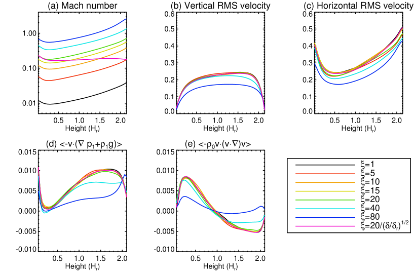
Figure 5: Some quantities averaged in time between $t=100$ and $200H_{\mathrm{r}}/v_{\mathrm{c}}$ in three dimensional calculation.(a) Distribution of Mach number estimated with the RMS velocity. (b) Distribution of vertical RMS velocity $v_{\mathrm{h}}$. (c) Distribution of horizontal RMS velocity. (d) Distribution of RMS power density of pressure and buoyancy. (e) Distribution of RMS power density of inertia.

References

- Brown et al. (2008) Brown, B. P., Browning, M. K., Brun, A. S., Miesch, M. S., & Toomre, J. 2008, ApJ, 689, 1354
- Brown et al. (2010) Brown, B. P., Browning, M. K., Brun, A. S., Miesch, M. S., & Toomre, J. 2010, ApJ, 711, 424
- Brown et al. (2011) Brown, B. P., Miesch, M. S., Browning, M. K., Brun, A. S., & Toomre, J. 2011, ApJ, 731, 69
- Brun et al. (2004) Brun, A. S., Miesch, M. S., & Toomre, J. 2004, ApJ, 614, 1073
- Choudhuri et al. (2007) Choudhuri, A. R., Chatterjee, P., & Jiang, J. 2007, Physical Review Letters, 98, 131103
- Choudhuri et al. (1995) Choudhuri, A. R., Schussler, M., & Dikpati, M. 1995, A&A, 303, L29
- Dikpati & Charbonneau (1999) Dikpati, M. & Charbonneau, P. 1999, ApJ, 518, 508
- Dikpati & Gilman (2006) Dikpati, M. & Gilman, P. A. 2006, ApJ, 649, 498
- Fan et al. (2003) Fan, Y., Abbett, W. P., & Fisher, G. H. 2003, ApJ, 582, 1206
- Gilman (1977) Gilman, P. A. 1977, Geophysical and Astrophysical Fluid Dynamics, 8, 93
- Gilman & Miller (1981) Gilman, P. A. & Miller, J. 1981, ApJS, 46, 211
- Glatzmaier (1984) Glatzmaier, G. A. 1984, Journal of Computational Physics, 55, 461
- Hotta & Yokoyama (2010a) Hotta, H. & Yokoyama, T. 2010a, ApJ, 709, 1009
- Hotta & Yokoyama (2010b) Hotta, H. & Yokoyama, T. 2010b, ApJ, 714, L308
- Hotta & Yokoyama (2011) Hotta, H. & Yokoyama, T. 2011, ApJ, 740, 12
- Kichatinov & Rüdiger (1993) Kichatinov, L. L. & Rüdiger, G. 1993, A&A, 276, 96
- Küker & Stix (2001) Küker, M. & Stix, M. 2001, A&A, 366, 668
- Miesch et al. (2006) Miesch, M. S., Brun, A. S., & Toomre, J. 2006, ApJ, 641, 618
- Miesch et al. (2000) Miesch, M. S., Elliott, J. R., Toomre, J., et al. 2000, ApJ, 532, 593
- Rempel (2005) Rempel, M. 2005, ApJ, 622, 1320
- Stix (2004) Stix, M. 2004, The sun : an introduction, 2nd edn., Astronomy and astrophysics library, (Berlin: Springer), ISBN: 3-540-20741-4
- Thompson et al. (2003) Thompson, M. J., Christensen-Dalsgaard, J., Miesch, M. S., & Toomre, J. 2003, ARA&A, 41, 599
- Yeates et al. (2008) Yeates, A. R., Nandy, D., & Mackay, D. H. 2008, ApJ, 673, 544