Phonon-limited transport coefficients in extrinsic graphene

Abstract

The effect of electron-phonon scattering processes over the thermoelectric properties of extrinsic graphene was studied. Electrical and thermal resistivity, as well as the thermopower, were calculated within the Bloch theory approximations. Analytical expressions for the different transport coefficients were obtained from a variational solution of the Boltzmann equation. The phonon-limited electrical resistivity $\rho_{e-ph}$ shows a linear dependence at high temperatures, and follows $\rho_{e-ph}\sim T^{4}$ at low temperatures, in agreement with experiments and theory previously reported in the literature. The phonon-limited thermal resistivity at low temperatures exhibits a $\sim T$ dependence, and achieves a nearly constant value at high temperatures. The predicted Seebeck coefficient at very low temperatures is $Q(T)\sim-\pi^{2}k_{B}^{2}T/(3\,e\,E_{F})$, which shows a $~{}n^{-1/2}$ dependence with the density of carriers, in agreement with experimental evidence. Our results suggest that thermoelectric properties can be controlled by adjusting the Bloch-Grüneisen temperature through its dependence on the extrinsic carrier density in graphene.

Recently, Efetov and Kim Efetov and Kim (2010) reported experimental measurements of the phonon-limited electrical resistivity of graphene samples, by achieving extremely high carrier densities by means of an electrolytic gate, in order to minimize the effect of other scattering mechanisms and to be away from the neutrality (Dirac) point. They observed that, at low temperatures, the electrical resistivity displays a $\sim T^{4}$ dependence, whereas at higher temperatures it follows a linear $\sim T$ trend, in agreement with an earlier theory by Hwang and Das Sarma Hwang and Das Sarma (2008). The later based their analysis on the Bloch theory Ziman (1960); Madelung (1978), which neglects phonon drag effects and umklapp processes, and modeled the interaction between electrons and longitudinal acoustic phonons by the deformation potential approximation. Moreover, they calculated the electrical resistivity Hwang and Das Sarma (2008) within the relaxation time approximation, which is valid for elastic scattering processes, a condition not strictly satisfied in electron-phonon scattering.

In this paper, phonon-limited transport coefficients in graphene are studied, by considering the presence of temperature and voltage gradients. Under similar assumptions as in Ref. (Hwang and Das Sarma (2008)), that is, Bloch theory and deformation potential approximation for the interaction between electrons and longitudinal-acoustic phonons, analytical expressions for the transport coefficients are obtained from a variational solution of the Boltzmann equation Ziman (1960); Madelung (1978). This method, at the lowest-order approximation, provides equivalent results to the relaxation time approximation and, at higher orders, converges to solutions of the Boltzmann equation which are exact to an arbitrary precision, within the limitations of the set of variational functions chosen. As has been pointed out before Peres and Lopes (2007), the semiclassical approach based on the Boltzmann equation cannot capture the subtleties of electronic transport in graphene right at the neutrality point. This limitation can, at least in part, be attributed to the inhomogeneity in the charge distribution experimentally observed in graphene samples at the neutrality pointPeres (2010). However, at high carrier densities the Fermi level is well above the Dirac point, and the Boltzmann equation then provides a correct description.

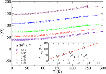
Figure 1: (Color online) Electrical resistivity calculated from Eq. (33) (lines), compared with experimental data (symbols) reported in Ref.(Efetov and Kim (2010)) at different carrier densities $n$ in units of $10^{17}m^{-2}$. Inset: Electrical resistivity at zero temperature, from data in Ref. (Efetov and Kim (2010)) (circles), at different carrier densities $n$. Also shown is the linear fit (dashed line) $\rho_{(T=0)}=14.276+266.17\times 10^{17}\,n^{-1}$ ($\Omega$) explained in the main text.

I Electron-phonon interaction

As is well known from tight-binding calculations, electronic transport in graphene displays relativistic features. This is because pristine graphene, free of impurities and defects, behaves as a metal only in the so-called Dirac points where the conduction and valence bands touch. There exists two non-equivalent such points within the first Brillouin zone, defined by the vectors $\mathbf{K}_{1,2}=\pm\frac{2\pi}{a}\left[1/\sqrt{3}\,,\,1\right]$, with $a$ the direct lattice parameter. In the vicinity of each of these points, or valleys, it is shown that the dispersion relation is linear, $E_{\eta}(\delta\mathbf{k})=\pm\hbar v_{F}|\delta\mathbf{k}|$, for $\delta\mathbf{k}=\mathbf{k}-\mathbf{K}_{\eta}$. In each valley $\mathbf{K}_{\eta}$, the envelope electronic functions related to this dispersion relation can thus be obtained as the pseudo-spinor solutions of an effective two-dimensional Dirac’s equation,

$$\hat{H}_{\mathbf{K}}\psi_{\mathbf{k}}^{(\pm)}=v_{F}\hat{\mathbf{\alpha}}\cdot\hat{\mathbf{p}}\psi_{\mathbf{k}}^{(\pm)}=E_{k}^{(\pm)}\psi_{\mathbf{k}}^{(\pm)}.$$ (1)

Here $\hat{\mathbf{\alpha}}=(\hat{\sigma}_{x},\hat{\sigma}_{y})$ are the Pauli matrices, we have re-defined $\mathbf{k}\equiv\delta\mathbf{k}$ for each valley, and the energy eigenvalues for positive (negative) helicity are $E_{k}^{(\pm)}=\pm\hbar v_{F}k$. The corresponding eigenvectors, normalized by the total area $A$ of the sample, are given by the pseudo-spinors

$$\psi_{\mathbf{k}}^{(\pm)}(\mathbf{r})=\frac{1}{\sqrt{2A}}\left(\begin{array}[]{c}e^{-i\varphi_{k}/2}\\ \pm e^{i\varphi_{k}/2}\end{array}\right)e^{i\mathbf{k}\cdot\mathbf{r}}\equiv u_{\mathbf{k}}^{(\pm)}\frac{e^{i\mathbf{k}\cdot\mathbf{r}}}{\sqrt{A}}$$ (4)

with $\varphi_{k}=\arctan(k_{y}/k_{x})$.

In the language of second quantization, the conduction electrons field for $\mathbf{k}$ in the vicinity of the $\mathbf{K}_{1,2}=\pm\frac{2\pi}{a}\left[1/\sqrt{3}\,,\,1\right]$ valley is

$$\hat{\psi}_{\eta}(\mathbf{r})=\sum_{\mathbf{k},\sigma}\psi_{\mathbf{k}}^{(+)}(\mathbf{r})\hat{c}_{\mathbf{k}\sigma\eta}$$ (5)

with $\hat{c}_{\mathbf{k}\sigma\eta}$ Fermionic operators $[\hat{c}_{\mathbf{k}\sigma\eta},\hat{c}_{\mathbf{k}^{\prime}\sigma^{\prime}\eta^{\prime}}^{\dagger}]_{+}=\delta_{\mathbf{k},\mathbf{k}^{\prime}}\delta_{\sigma,\sigma^{\prime}}\delta_{\eta,\eta^{\prime}}$, that destroy (create) a conduction electron with momentum $\hbar\mathbf{k}$ in the vicinity of the $\mathbf{K}_{\eta}$ valley, with spin component $\sigma=\{\uparrow,\downarrow\}$. We model the electron-phonon interaction by the deformation potential approximation Hwang and Das Sarma (2008), which is a reasonable one when the Fermi surface possesses spherical symmetry Ziman (1960); Madelung (1978). The two-dimensional version of this is a Fermi ”circle” in graphene, which corresponds to the intersection of the Dirac cone and the constant energy plane defined by the Fermi energy at $\epsilon_{k}=E_{F}$. In the deformation potential approximation, the operator representing lattice dilation in the second quantization language is

$$\hat{\Delta}(\mathbf{r})=i\sum_{\mathbf{q}}\left(2A\rho_{m}\omega_{q}\right)^{-1/2}(\mathbf{q}\cdot\hat{e}_{L})\left(\hat{a}_{q}^{\dagger}e^{i\mathbf{q}\cdot\mathbf{r}}-\hat{a}_{q}e^{-i\mathbf{q}\cdot\mathbf{r}}\right)$$ (6)

Here, $\omega_{q}=v_{s}q$ is the frequency for longitudinal acoustic phonons in graphene, $\hat{a}^{\dagger}_{q}$ is the creation operator for longitudinal acoustic phonon modes, and $\hat{e}_{L}$ is the corresponding polarization vector for these modes. The electron-phonon interaction Hamiltonian, in the deformation potential approximation, is obtained from

$$\hat{H}^{int}_{e-ph}=i\int{d^{2}r}\sum_{\eta=1,2}\hat{\psi}^{\dagger}_{\eta}(\mathbf{r})D\hat{\Delta}(\mathbf{r})\hat{\psi}_{\eta}(\mathbf{r})$$ (7)

$$=i\sum_{\mathbf{k},\mathbf{q},\eta,\sigma}\sqrt{\frac{\hbar q^{2}D^{2}}{2\rho_{m}\omega_{q}}}\cos\left(\theta/2\right)\left(\hat{a}_{\mathbf{q}}-\hat{a}_{-\mathbf{q}}^{\dagger}\right)\hat{c}^{\dagger}_{\mathbf{k}+\mathbf{q},\sigma\eta}\hat{c}_{\mathbf{k}\sigma\eta}$$

Notice the presence of the factor $\cos(\theta/2)=\cos([\varphi_{k}-\varphi_{k^{\prime}}]/2)$ which arises from the inner product of the two pseudo-spinor functions $u_{\mathbf{k}^{\prime}}^{*}\cdot u_{\mathbf{k}}$ defined in Eq. (4). This factor, which would be absent from the inner product of non-relativistic scalar Schrödinger wave-functions, is a fingerprint of the relativistic features of electrons in graphene. The more obvious consequence of its presence the suppression of backscattering ($\theta=\pi$), a phenomenon observed in graphene and directly related to so called Klein tunneling Beenakker (2008); Peres (2010); Castro, Guinea and Peres (2009) in the context of relativistic quantum mechanics.

We shall neglect umklapp processes, and thus we have $\mathbf{G}=0$ for normal processes. In this case, scattering events satisfy energy and ”crystal momentum” conservation, $\epsilon_{k^{\prime}}=\epsilon_{k}\pm\hbar\omega_{q}$ and $\mathbf{k}^{\prime}=\mathbf{k}\pm\mathbf{q}$. From the latter equation, one obtains the condition $q^{2}=k^{\prime 2}+k^{2}-2kk^{\prime}cos(\theta)$, with $\theta$ the scattering angle. Since the relevant scattering events occur within a thin layer near the Fermi surface, then $k\sim k^{\prime}\sim k_{F}$, which then implies $\left|sin(\theta/2)\right|=q/2k_{F}$. In a Debye model approximation, this condition restricts the range of lattice momenta involved in electron-phonon scattering, $q\leq\min\{2k_{F},q_{D}\}$, with $q_{D}$ the radius of the Debye circle (for a two-dimensional system). In geometrical terms, the most restrictive condition depends on whether the radius of the Fermi surface (a circle centered on each Dirac point for graphene) is larger or smaller than the Debye circle. When written in terms of the frequency of the longitudinal-acoustic phonon modes involved $\omega_{q}=v_{s}q$, the former condition reads $\hbar\omega_{q}/k_{B}\leq\min\{\Theta_{BG},\Theta_{D}\}$, with $\Theta_{D}$ the Debye temperature, and $\Theta_{BG}=2(v_{s}/v_{F})E_{F}/k_{B}$ the Bloch-Grüneisen temperature. In the experimental setup presented in Ref.(Efetov and Kim (2010)), the carrier densities involved are such that the Fermi surface is contained within the Debye circle, and therefore the Bloch-Grüneisen rather than the Debye temperature imposes the characteristic energy scale for phonon scatterers. Notice that the analysis of the scattering angle above also yields the relation $\cos(\theta/2)=\sqrt{1-(q/(2k_{F}))^{2}}$. Therefore, after Eq. (I) the matrix element for the electron-phonon interaction $\hat{H}_{e-ph}^{int}=i\sum_{\mathbf{k},\mathbf{q},\eta,\sigma}M_{\mathbf{q}}\left(\hat{a}_{\mathbf{q}}-\hat{a}_{-\mathbf{q}}^{\dagger}\right)\hat{c}^{\dagger}_{\mathbf{k}+\mathbf{q},\sigma\eta}\hat{c}_{\mathbf{k}\sigma\eta}$ is

$$M_{q}=-i\left(\hbar/2\rho_{m}\omega_{q}\right)^{1/2}Dq\left(1-\left(q/2k_{F}\right)^{2}\right)^{1/2}.$$ (8)

Here, $D$ is the deformation potentialZiman (1960); Madelung (1978); Efetov and Kim (2010) coupling constant for graphene, and $\rho_{m}=7.6\times 10^{-7}$ kg/$\rm{m}^{2}$ the surface mass density.

II Boltzmann Equation

We introduce, in the usual form, the deviation of the distribution function from equilibrium by the expression $f_{k}=f_{k}^{0}-\chi_{\mathbf{k}}\partial f_{k}^{0}/\partial\epsilon_{k}$. Let us consider the electron-phonon interaction as the sole scattering mechanism. Therefore, after Eqs.(5,8) we should consider processes of the form $\mathbf{k}+\mathbf{q}\rightleftarrows\mathbf{k}^{\prime}$. Under Bloch’s approximation, which is to assume that the phonon system is in quasi-equilibrium, the linearized form of the Boltzmann equation when both an external electric field and a temperature gradient are imposed can be expressed as

$$-\mathbf{v}_{\mathbf{k}}\cdot\nabla T\frac{\partial f_{k}^{0}}{\partial T}-\mathbf{v}_{\mathbf{k}}\cdot\mathbf{E}(-e)\frac{\partial f_{k}^{0}}{\partial\epsilon_{k}}=$$

$$\frac{g_{\eta}g_{\sigma}}{k_{B}T}\sum_{\mathbf{k}^{\prime},\mathbf{q}}\left[\{\chi_{\mathbf{k}}-\chi_{\mathbf{k}^{\prime}}\}\mathcal{P}_{\mathbf{k}\mathbf{q}}^{\mathbf{k}^{\prime}}-\{\chi_{\mathbf{k}^{\prime}}-\chi_{\mathbf{k}}\}\mathcal{P}^{\mathbf{k}\mathbf{q}}_{\mathbf{k}^{\prime}}\right]$$ (9)

Here, $g_{\eta}=g_{\sigma}=2$ are the spin and valley degeneracies, respectively, while the transition rate for electron-phonon scattering processes is

$$\mathcal{P}_{\mathbf{k}\mathbf{q}}^{\mathbf{k}^{\prime}} =\left(2\pi/\hbar\right)\delta_{\mathbf{G},\mathbf{k}^{\prime}-\mathbf{k}-\mathbf{q}}|M_{q}|^{2}\delta(\epsilon_{k}-\epsilon_{k^{\prime}}+\hbar\omega_{q})$$ (10)

$$\times n_{q}^{0}f_{k}^{0}(1-f^{0}_{k^{\prime}})$$

Here $f_{k}^{0}$ is the Fermi-Dirac distribution for electron states with momentum $\mathbf{k}$, and $n_{q}^{0}$ the Bose distribution for phonon states with momentum $\mathbf{q}$. All vectors are two-dimensional, with $\mathbf{G}$ a vector of the reciprocal lattice.

For extrinsic graphene, the Fermi level $E_{F}=\hbar k_{F}v_{F}$ is located above the Dirac point, and depends on the density of carriers $n$ by the relation $k_{F}=\sqrt{\pi n}$. In Ref.(Efetov and Kim (2010)), an experimental method is presented which allows to control the carrier density, and hence the Bloch-Grüneisen temperature. As discussed in Refs.(Efetov and Kim (2010); Fuhrer (2010)), this in turn becomes a way to control the phonon-limited electrical resistivity. In this work, we will show that also the electronic component of the thermal conductivity, as well as the thermopower (Seebeck coefficient) which determines thermoelectric effects, can be controlled in a similar way. We shall use the variational method to calculate the phonon-limited transport coefficients which, in contrast with the relaxation time approximation, it has the advantage of avoiding the assumption of quasi-elasticity in the scattering processes.

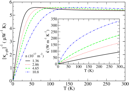
Figure 2: (Color online) Phonon-limited thermal resistivity $[\kappa_{e-ph}]^{-1}$, calculated from Eq.(36) at different carrier densities $n$, in units of $10^{17}m^{-2}$. Shown in the inset is the corresponding thermal conductivity, including the contribution from Coulomb elastic scattering with impurities, and normalized with a nominal packing thickness of $3.4$ Å.

III Coupled charge and heat transport

For a system with thermal and electrostatic potential gradients, the macroscopic entropy production rate is given in terms of the heat $\mathbf{U}$ and charge $\mathbf{J}$ fluxes by Ziman (1960); Madelung (1978)

$$\partial_{t}S=\mathbf{J}\cdot\mathbf{E}/T+\mathbf{U}\cdot\nabla\left(1/T\right).$$ (11)

The Onsager’s theorem Onsager (1931) indicates that the fluxes and generalized potentials are then linearly coupled,

$$\mathbf{J}=L_{EE}\mathbf{E}+L_{ET}\nabla T$$

$$\mathbf{U}=L_{TE}\mathbf{E}+L_{TT}\nabla T$$ (12)

The thermopower $Q$ can be expressed in terms of the coefficients $L_{\alpha\beta}$ by considering the case $\mathbf{J}=0$ in Eq. (12), to obtain $\mathbf{E}=-L_{ET}L_{EE}^{-1}\nabla T$. Hence, one concludes that $Q=-L_{ET}L_{EE}^{-1}$. The thermal conductivity is obtained from the second equation, $\mathbf{U}=-(L_{TE}L_{EE}^{-1}L_{ET}-L_{TT})\nabla T$, which implies $\kappa=L_{TE}L_{EE}^{-1}L_{ET}-L_{TT}$. If, on the other hand, one considers the case $\nabla T=0$, then the relation $\mathbf{J}=L_{EE}\mathbf{E}$ is obtained. Thus, it is concluded that the electrical resistivity is $\rho=L_{EE}^{-1}$. The variational method Ziman (1960); Madelung (1978) is based on the principle of maximal entropy production Onsager (1931), and provides an iterative but virtually exact procedure to solve the Boltzmann equation, and therefore to calculate the transport coefficients, within the limitations of the set of variational functions chosen. The principle is based on equating the macroscopic entropy production rate, as expressed in terms of the macroscopic currents Eq.(12), with the entropy production rate due to microscopic scattering eventsOnsager (1931), $\partial_{t}S=\dot{S}_{scatt}$, as defined from the linearized Boltzmann equation scattering terms,

$$\dot{S}_{scatt}=\frac{g_{\eta}g_{\sigma}}{k_{B}T^{2}}\sum_{\mathbf{k},\mathbf{q},\mathbf{k}^{\prime}}\{\chi_{\mathbf{k}}-\chi_{\mathbf{k}^{\prime}}\}^{2}\mathcal{P}_{\mathbf{k}\mathbf{q}}^{\mathbf{k}^{\prime}}$$ (13)

The electric current $\mathbf{J}$ and the heat current $\mathbf{U}$ are given by the expressions

$$\mathbf{J} = g_{\eta}g_{\sigma}\sum_{\mathbf{k}}(-e)\mathbf{v}_{\mathbf{k}}\chi_{\mathbf{k}}\frac{\partial f_{k}^{0}}{\partial\epsilon_{k}}$$

$$\mathbf{U} = g_{\eta}g_{\sigma}\sum_{\mathbf{k}}\mathbf{v}_{\mathbf{k}}(\epsilon_{k}-E_{F})\chi_{\mathbf{k}}\frac{\partial f_{k}^{0}}{\partial\epsilon_{k}}$$ (14)

The technique is based on expanding the distribution function deviation from equilibrium $\chi_{\mathbf{k}}=\sum_{i}\alpha_{i}\phi_{i}(\mathbf{k})$ in terms of a set of variational functions of the form $\phi_{i}(\mathbf{k})=(\epsilon_{k}-E_{F})^{i-1}(\hat{u}\cdot\mathbf{k})$. For a minimal set of trial functions $\phi_{1}(\mathbf{k})=\mathbf{k}\cdot\hat{u}$ and $\phi_{2}(\mathbf{k})=\mathbf{k}\cdot\hat{u}(\epsilon_{k}-E_{F})$, we obtain the charge and heat currents

$$\mathbf{J}_{i} =(-e)g_{\eta}g_{\sigma}\sum_{\mathbf{k}}\mathbf{v}_{\mathbf{k}}\phi_{i}(\mathbf{k})\frac{\partial{f}^{0}}{\partial\epsilon_{k}}$$

$$\mathbf{U}_{i} =g_{\eta}g_{\sigma}\sum_{\mathbf{k}}\mathbf{v}_{\mathbf{k}}(\epsilon_{k}-E_{F})\phi_{i}(\mathbf{k})\frac{\partial{f}^{0}}{\partial\epsilon_{k}}$$ (15)

Here, $g_{\eta}=g_{\sigma}=2$ are the valley and spin degeneracies in graphene, respectively. The coefficients $P_{ij}=P_{ji}$ are defined as follows

$$P_{ij}=\frac{(g_{\eta}g_{\sigma})^{2}}{k_{B}T}\sum_{\mathbf{k},\mathbf{k}^{\prime},\mathbf{q}}\{\phi_{i}(\mathbf{k})-\phi_{i}(\mathbf{k}^{\prime})\}\{\phi_{j}(\mathbf{k})-\phi_{j}(\mathbf{k}^{\prime})\}\mathcal{P}_{\mathbf{k}\mathbf{q}}^{\mathbf{k}^{\prime}}$$

(16)

In terms of the variational solution, after Eq.(14) the electric and heat currents are written as

$$\mathbf{J} = \sum_{i}\alpha_{i}\mathbf{J}_{i}$$

$$\mathbf{U} = \sum_{i}\alpha_{i}\mathbf{U}_{i}$$ (17)

whereas the macroscopic $\partial_{t}S$ and microscopic $\dot{S}_{scatt}$ entropy generation rates in Eqs.(11,13) are expressed by

$$\partial_{t}S = \sum_{i}\alpha_{i}\left[T^{-1}\mathbf{J}_{i}\cdot\mathbf{E}-T^{-2}\mathbf{U}_{i}\cdot\mathbf{\nabla}T\right],$$

$$\dot{S}_{scatt} = T^{-1}\sum_{i,j}\alpha_{i}\alpha_{j}P_{ij}.$$ (18)

The variational problem is to find the set of coefficients $\{\alpha_{j}\}$ that maximize $\dot{S}_{scatt}$, subject to the constraint $\partial_{t}S=\dot{S}_{scatt}$, which is enforced by a Lagrange multiplier $\lambda$,

$$\frac{\delta}{\delta\alpha_{n}}\left[\sum_{i,j}\alpha_{i}\alpha_{j}\frac{P_{ij}}{T}-\lambda\,\,\sum_{i}\alpha_{i}\left(\frac{\mathbf{J}_{i}\cdot\mathbf{E}}{T}-\mathbf{U}_{i}\cdot\frac{\mathbf{\nabla}T}{T^{2}}\right)\right]=0$$

(19)

The solution to this constrained variational problem is given by $\lambda=1/2$, and

$$\alpha_{i}=\sum_{j}[P^{-1}]_{ij}\left(\mathbf{J}_{j}\cdot\mathbf{E}-\mathbf{U}_{j}\cdot\frac{\nabla T}{T}\right)$$ (20)

Here, $[P^{-1}]$ is the inverse of the matrix $[P]_{ij}=P_{ij}$ whose elements are the coefficients $P_{ij}$ defined by Eq.(16). After substituting this solution into the expressions for the electric and heat currents, we obtain explicit analytical formulas for the transport coefficient tensors defined in Eq.(12),

$$L_{EE} = \sum_{ij}\mathbf{J}_{i}[P^{-1}]_{ij}\mathbf{J}_{j}$$

$$L_{ET} = -T^{-1}\sum_{ij}\mathbf{J}_{i}[P^{-1}]_{ij}\mathbf{U}_{j}$$

$$L_{TE} = \sum_{ij}\mathbf{U}_{i}[P^{-1}]_{ij}\mathbf{J}_{j}$$

$$L_{TT} = -T^{-1}\sum_{ij}\mathbf{U}_{i}[P^{-1}]_{ij}\mathbf{U}_{j}$$ (21)

Therefore, we proceed to calculate the currents and $P_{ij}$ coefficients. Let us first consider the current $\mathbf{J}_{1}$. The group velocity in Eq.(15) is given by $\mathbf{v}_{\mathbf{k}}=\hat{k}v_{F}$, with $\hat{k}=\mathbf{k}/k=(\cos(\varphi),\sin(\varphi))$. The discrete sums are treated in the usual quasi-continuum limit as two-dimensional integrals, $\sum_{\mathbf{k}}\rightarrow A(2\pi)^{-2}\int d^{2}k$, and the integral is calculated by using the change of variables $d^{2}k=d\varphi\epsilon d\epsilon/(\hbar v_{F})^{2}$,

$$\mathbf{J}_{1} =\frac{A(-e)v_{F}}{\pi^{2}(\hbar v_{F})^{3}}\int_{-\pi}^{+\pi}d\varphi\hat{k}\hat{k}\cdot\hat{u}\int d\epsilon\epsilon^{2}\frac{\partial f_{\epsilon}^{0}}{\partial\epsilon}$$ (22)

$$=\hat{u}\frac{Ae}{\pi\hbar}\left(\frac{E_{F}}{\hbar v_{F}}\right)^{2}$$

For the current $\mathbf{U}_{1}$, we consider the quasi-continuum limit for the sum over wave-vectors in Eq.(15), with directions $\hat{k}=\mathbf{k}/k=(\cos(\varphi),\sin(\varphi))$. Using the integration variables $d^{2}k=d\varphi d\epsilon\epsilon/(\hbar v_{F})^{2}$, we have

$$\mathbf{U}_{1} = \frac{Av_{F}}{\pi^{2}(\hbar v_{F})^{3}}\int_{-\pi}^{\pi}d\varphi\hat{k}\hat{k}\cdot\hat{u}\int d\epsilon\epsilon^{2}(\epsilon-E_{F})\left(\frac{\partial f_{\epsilon}^{0}}{\partial\epsilon}\right)$$ (23)

$$= -\hat{u}\frac{2\pi A}{3}\frac{(k_{B}T)^{2}}{\hbar}\frac{E_{F}}{(\hbar v_{F})^{2}}$$

Similarly, for the current $\mathbf{U}_{2}$ we obtain

$$\mathbf{U}_{2} = \frac{Av_{F}}{\pi^{2}(\hbar v_{F})^{3}}\int_{-\pi}^{\pi}d\varphi\hat{k}\hat{k}\cdot\hat{u}\int d\epsilon\epsilon^{2}(\epsilon-E_{F})^{2}\left(\frac{\partial f_{\epsilon}^{0}}{\partial\epsilon}\right)$$ (24)

$$= -\hat{u}\frac{\pi A}{3}\frac{(k_{B}T)^{2}}{\hbar}\left(\frac{E_{F}}{\hbar v_{F}}\right)^{2}$$

Finally, it is straightforward to verify by inspection that $\mathbf{J}_{2}=(-e)\mathbf{U}_{1}$.

Let us now consider the coefficient $P_{11}$. From Eq.(10), we first notice that the transition probability rate $\mathcal{P}_{\mathbf{k}\mathbf{q}}^{\mathbf{k}^{\prime}}$ imposes the condition $\mathbf{q}=\mathbf{k}^{\prime}-\mathbf{k}$. We define the directions $\hat{k}^{\prime}=(\cos(\varphi^{\prime}),\sin(\varphi^{\prime}))$ and $\hat{k}=(\cos(\varphi^{\prime}-\theta),\sin(\varphi^{\prime}-\theta))$, with $\theta$ the scattering angle. As before, in the quasi-continuum limit for the sums over wave-vectors, we choose the integration variables $d^{2}kd^{2}k^{\prime}=d\varphi^{\prime}d\theta d\epsilon^{\prime}\epsilon^{\prime}d\epsilon\epsilon/(\hbar v_{F})^{4}$, to obtain

$$P_{11} =\frac{(k_{B}T)^{-1}A^{2}}{(\pi\hbar v_{F})^{4}}\int d\epsilon\epsilon\int d\epsilon^{\prime}\epsilon^{\prime}$$ (25)

$$\times\int_{-\pi}^{\pi}d\theta\int_{-\pi}^{\pi}d\varphi^{\prime}(\mathbf{q}\cdot\hat{u})^{2}\mathcal{P}_{\mathbf{k}\mathbf{q}}^{\mathbf{k}^{\prime}}$$

In Appendix A it is shown that the angular integral $\int d\varphi^{\prime}(\mathbf{q}\cdot\hat{u})^{2}=\pi q^{2}$, with $q=2k_{F}\sin(\theta/2)$. Hence, substituting the explicit expression for the transition probability rate, Eq.(25) reduces to

$$\frac{2(k_{B}T)^{-1}A^{2}}{\pi^{2}\hbar(\hbar v_{F})^{4}}\int_{-\pi}^{\pi}d\theta q^{2}n_{q}^{0}|M_{q}|^{2}$$

$$\times\int d\epsilon\epsilon(\epsilon+\hbar\omega_{q})f_{\epsilon}^{0}(1-f_{\epsilon+\hbar\omega_{q}}^{0})$$ (26)

The energy integral is evaluated using the technique presented in Appendix B. Using the change of variables $d\theta=k_{F}^{-1}[1-(q/(2k_{F}))^{2}]^{-1/2}dq$, we obtain

$$P_{11}=\frac{(k_{B}T)^{-1}A^{2}k_{F}\hbar D^{2}}{\pi^{2}\rho_{m}(\hbar v_{F})^{2}}\int_{0}^{2k_{F}}dq\left(q^{4}+4\left(\frac{v_{s}}{v_{F}}\right)^{2}\right.$$

$$\times\left.\left(\frac{T}{\Theta_{BG}}\right)^{2}\left[\frac{\pi^{2}q^{4}}{3}+\frac{q^{6}}{2}\right][1-\left(\frac{q}{2k_{F}}\right)^{2}]^{1/2}\right)$$

$$\times(1-e^{-\hbar\omega_{q}/(k_{B}T)})^{-1}(e^{\hbar\omega_{q}/(k_{B}T)}-1)^{-1}$$ (27)

Eq.(27) is written in terms of the functions $\mathcal{J}_{p}(z)$ defined in Appendix C,

$$P_{11}=\frac{\hbar D^{2}A^{2}E_{F}(k_{B}T)^{4}}{\pi^{2}\rho_{m}(\hbar v_{s})^{5}(\hbar v_{F})^{3}}\left[\mathcal{J}_{4}(T/\Theta_{BG})+4\left(\frac{v_{s}}{v_{F}}\right)^{2}\right.$$

$$\left.\times\left(\frac{T}{\Theta_{BG}}\right)^{2}\left\{\frac{\pi^{2}}{3}\mathcal{J}_{4}(T/\Theta_{BG})+\frac{1}{2}\mathcal{J}_{6}(T/\Theta_{BG})\right\}\right]$$ (28)

Let us now consider the coefficient $P_{22}$, which after similar manipulations as before, can be expressed by the integral form

$$P_{22} =\frac{(k_{B}T)^{-1}A^{2}}{(\pi\hbar v_{F})^{4}}\int_{-\pi}^{\pi}d\theta\int_{-\pi}^{\pi}d\varphi^{\prime}\int d\epsilon\epsilon\int d\epsilon^{\prime}\epsilon^{\prime}$$ (29)

$$\times[(\mathbf{q}\cdot\hat{u})(\epsilon-E_{F})+\hbar\omega_{q}(\mathbf{k}^{\prime}\cdot\hat{u})]^{2}\mathcal{P}_{\mathbf{k}\mathbf{q}}^{\mathbf{k}^{\prime}}$$

After expanding the square in Eq.(29), it is shown in Appendix A that the angular integrals give, $\int d\varphi^{\prime}(\mathbf{q}\cdot\hat{u})^{2}=\pi q^{2}$, $\int d\varphi^{\prime}(\mathbf{k}^{\prime}\cdot\hat{u})=\pi k^{\prime 2}$, and $\int d\varphi^{\prime}(\mathbf{q}\cdot\hat{u})(\mathbf{k}^{\prime}\cdot\hat{u})=(\pi/2)[q^{2}+k^{\prime 2}-k^{2}]$. Then, after similar algebraic procedures as described previously, Eq.(29) reduces to

$$P_{22}=\frac{\hbar D^{2}A^{2}E_{F}^{3}(k_{B}T)^{4}}{\pi^{2}\rho_{m}(\hbar v_{s})^{3}(\hbar v_{F})^{5}}\left[\left\{1+\frac{4\pi^{2}}{3}\left(1+12\right.\right.\right.$$

$$\left.\left.\left.\times\left(\frac{v_{s}}{v_{F}}\right)^{2}\right)\right\}\left(\frac{T}{\Theta_{BG}}\right)^{2}\mathcal{J}_{4}(T/\Theta_{BG})-\frac{2}{3}\left\{1-6\right.\right.$$

$$\left.\left.\times\left(\frac{v_{s}}{v_{F}}\right)^{2}\right\}\left(\frac{T}{\Theta_{BG}}\right)^{2}\mathcal{J}_{6}(T/\Theta_{BG})+\frac{16\pi^{2}}{3}\left(\frac{v_{s}}{v_{F}}\right)^{2}\right.$$

$$\left.\times\left(\frac{T}{\Theta_{BG}}\right)^{4}\left\{\left(\frac{v_{s}}{v_{F}}\right)^{2}\mathcal{J}_{6}(T/\Theta_{BG})+\frac{1}{10\pi^{2}}\left\{1\right.\right.\right.$$

$$\left.\left.\left.-2\left(\frac{v_{s}}{v_{F}}\right)^{2}\right\}\mathcal{J}_{8}(T/\Theta_{BG})\right\}\right]$$ (30)

At last, we consider the coefficient $P_{12}$. After our definition Eq.(16), we have

$$P_{12} =\frac{(k_{B}T)^{-1}A^{2}}{(\pi\hbar v_{F})^{4}}\int_{-\pi}^{\pi}d\theta\int_{-\pi}^{\pi}d\varphi^{\prime}\int d\epsilon\epsilon\int d\epsilon^{\prime}\epsilon^{\prime}$$ (31)

$$\times[(\mathbf{q}\cdot\hat{u})^{2}(\epsilon-E_{F})+\hbar\omega_{q}(\mathbf{k}^{\prime}\cdot\hat{u})(\mathbf{q}\cdot\hat{u})]\mathcal{P}_{\mathbf{k}\mathbf{q}}^{\mathbf{k}^{\prime}}$$

As shown in Appendix A, the angular integrals are given by $\int d\varphi^{\prime}(\mathbf{q}\cdot\hat{u})^{2}=\pi q^{2}$, and $\int d\varphi^{\prime}(\mathbf{q}\cdot\hat{u})(\mathbf{k}^{\prime}\cdot\hat{u})=(\pi/2)[q^{2}+k^{\prime 2}-k^{2}]$. Therefore, using the procedure described previously, the integral in Eq.(31) is calculated and expressed in terms of the $\mathcal{J}_{p}(z)$ functions defined in Appendix C,

$$P_{12}=\frac{\hbar D^{2}A^{2}E_{F}^{2}(k_{B}T)^{4}}{\pi^{2}\rho_{m}(\hbar v_{s})^{3}(\hbar v_{F})^{5}}\left[\mathcal{J}_{4}(T/\Theta_{BG})-\frac{v_{s}}{v_{F}}\left(\frac{T}{\Theta_{BG}}\right)\right.$$

$$\left.\times\mathcal{J}_{5}(T/\Theta_{BG})+\frac{8\pi^{2}}{3}\left(\frac{T}{\Theta_{BG}}\right)^{2}\left\{\mathcal{J}_{4}(T/\Theta_{BG})+\frac{3}{2}\right.\right.$$

$$\left.\left.\times\left(\frac{v_{s}}{v_{F}}\right)^{2}\mathcal{J}_{4}(T/\Theta_{BG})+\frac{1}{4\pi^{2}}\mathcal{J}_{6}(T/\Theta_{BG})\right\}+\frac{2}{3}\right.$$ (32)

$$\left.\times\left(\frac{v_{s}}{v_{F}}\right)^{3}\left(\frac{T}{\Theta_{BG}}\right)^{3}\left\{\mathcal{J}_{7}(T/\Theta_{BG})-2\pi^{2}\mathcal{J}_{5}(T/\Theta_{BG})\right\}\right]$$

IV Electrical Resistivity

As discussed in Section III, the electrical resistivity is obtained by setting $\nabla T=0$ in Eq. (12), to obtain $\rho=L_{EE}^{-1}$. By direct substitution of the coefficients and currents obtained in Section III, we obtain after Eqs.(21) that the leading term which defines the electrical resistivity due to electron-phonon scattering processes is

$$\rho_{e-ph}(T)=\rho_{0}\left[\left(\frac{T}{\Theta_{BG}}\right)^{4}{\mathcal{J}}_{4}(\Theta_{BG}/T)+\frac{4\pi^{2}}{3}\left(\frac{v_{s}}{v_{F}}\right)^{2}\right.$$

$$\left.\times\left(\frac{T}{\Theta_{BG}}\right)^{6}\left\{{\mathcal{J}}_{4}(\Theta_{BG}/T)+\frac{3}{2\pi^{2}}{\mathcal{J}}_{6}(\Theta_{BG}/T)\right\}\right]$$ (33)

Here, $\rho_{0}=8\,D^{2}k_{F}/(e^{2}\rho_{m}v_{s}v_{F}^{2})$ is a coefficient with dimensions of a two-dimensional resistivity ($\Omega$), and $\Theta_{BG}=2(v_{s}/v_{F})E_{F}/k_{B}$ is the Bloch-Grüneisen temperature. The functions ${\mathcal{J}}_{p}(\Theta_{BG}/T)$ and their asymptotic properties are defined in Appendix C. Eq. (33) depends on the dimensionless parameter $T/\Theta_{BG}$, a feature previously obtainedHwang and Das Sarma (2008) within the relaxation time approximation. The functions ${\mathcal{J}}_{p}(\Theta_{BG}/T)$, defined in Appendix C, have the property ${\mathcal{J}}_{p}(\infty)=p!\zeta(p)$, with $\zeta(p)$ the Riemann zeta function. Therefore, the low-temperature ($T\ll\Theta_{BG}$) behavior of the electron-phonon contribution to the electrical resistivity is

$$\rho_{e-ph}(T) =\rho_{0}\,4!\zeta(4)(T/\Theta_{BG})^{4}+o(T/\Theta_{BG})^{6}$$ (34)

At high temperature ($T\gg\Theta_{BG}$), from Eq.(33) we find the asymptotic limit $\rho_{e-ph}(T)=\{1/3-1/10\ldots\}\rho_{0}\,T/\Theta_{BG}=(\pi/8)\rho_{0}\,T/\Theta_{BG}$. This behavior is in agreement with experiments Efetov and Kim (2010) and earlier theoretical results based on the relaxation time approximation Hwang and Das Sarma (2008), thus supporting the application of the variational method in this case. In Fig.(1) we compare the theoretical prediction with the experimental data reported in Ref. (Efetov and Kim (2010)). The experimental data are fitted to the expression

$$\rho(T)=\rho_{(T=0)}+\rho_{e-ph}(T),$$ (35)

with $\rho_{e-ph}(T)$ defined by our theory Eq.(33), and $\rho_{(T=0)}$ being the value of the resistivity at zero temperature. This parameter can be interpreted as the (temperature independent) contribution of impurity scattering to the total electrical resistivity. The impurity contribution to the electrical resistivity has been discussed Stauber, Peres and Guinea (2007); Peres and Lopes (2007), and it is a sample-dependent property, since it is proportional to the surface concentration of impurities $n_{imp}$. It has been shown Stauber, Peres and Guinea (2007); Peres and Lopes (2007) that, for a short range scattering potential $V_{scatt}(\mathbf{r})=V_{0}\delta(\mathbf{r})$, the in-plane resistivity is $\rho_{scatt}\propto n_{imp}V_{0}^{2}$, whereas for a long range Coulomb potential Stauber, Peres and Guinea (2007) $\rho_{scatt}\propto n_{imp}n^{-1}$, this last case showing an inverse dependency on the carrier concentration $n$ as well. Therefore, it is expected that the zero temperature resistivity exhibits a dependence on the carrier concentration of the form $\rho_{(T=0)}=a+bn^{-1}$, with the value of the coefficients $a$ and $b$ depending on details of the sample, particularly on the concentration and distribution of impurities and defects. We verify that this equation is in excellent agreement with the data reported in Ref. (Efetov and Kim (2010)), as shown in the inset of Fig. (1). We extracted values $a=14.276$ ($\Omega$) and $b=266.76\times 10^{17}$ ($\Omega\,\rm{m^{2}}$), with linear regression coefficient $r=0.999$.

As seen in Fig. (1), Eq.(35) provides an excellent fit to the experimental data. The temperature-dependent electron-phonon contribution to the electrical resistivity is fitted with just two free parameters: The energy parameter $D=23.5\pm 0.5$ eV in the deformation potential, and the speed of sound for longitudinal phonons in graphene $v_{s}=24.0\pm 0.6$ Km/s. It is remarkable that both values are in excellent agreement with independent estimations reported in the literature, particularly the speed of sound Munoz and Lu (2010); Saito Dresselhaus (1998). It is also relevant to notice that the ratio $(v_{s}/v_{F})^{2}\sim 10^{-4}$ is negligibly small, and hence terms proportional to this factor can in practice be neglected in the analytical expressions obtained for the electrical resistivity, as well as in other transport coefficients discussed along this work. This also explains the quantitative success when applying the relaxation time approximation to electron-phonon scattering as reported in previous theoretical work Hwang and Das Sarma (2008), even though this scattering mechanism is not strictly quasi-elastic.

V Thermal Resistivity

The thermal conductivity is obtained from the general expression Eq. (12) by setting $\mathbf{J}=0$, which as discussed in Section III leads to the expression $\kappa=L_{TE}L_{EE}^{-1}L_{ET}-L_{TT}$. By direct substitution of the coefficients and currents calculated in Section III, and neglecting terms proportional to $(v_{s}/v_{F})^{2}\sim 10^{-4}$, we obtain that the leading contribution to the thermal resistivity due to electron-phonon scattering is given by

$$[\kappa_{e-ph}(T)]^{-1}=\frac{\rho_{0}}{{\mathcal{L}}_{0}T}\left\{\left[\left(T/\Theta_{BG}\right)^{4}+\frac{3}{4\pi^{2}}(T/\Theta_{BG})^{2}\right]\right.$$

$$\times\left.{\mathcal{J}}_{4}(\Theta_{BG}/T)-\frac{1}{2\pi^{2}}\left(T/\Theta_{BG}\right)^{4}{\mathcal{J}}_{6}(\Theta_{BG}/T)\right\}$$ (36)

Here, ${\mathcal{L}}_{0}=\pi^{2}k_{B}^{2}/(3\,e^{2})$ is the Lorenz number for the free electron gas. At very low temperatures ($T\ll\Theta_{BG}$), Eq. (36) predicts the asymptotic limit

$$[\kappa_{e-ph}(T)]^{-1}=\frac{\rho_{0}}{{\mathcal{L}}_{0}\Theta_{BG}}\frac{3}{4\pi^{2}}4!\zeta(4)\frac{T}{\Theta_{BG}}+o\left(\frac{T}{\Theta_{BG}}\right)^{3}$$ (37)

It is remarkable that, according to Eq. (37), the phonon-limited thermal resistivity is linear at very low temperatures, in contrast with the typical $\sim T^{2}$ behavior theoretically predicted and experimentally observed in normal, three-dimensional metals Ziman (1960); Madelung (1978). The thermal resistivity contribution due to elastic scattering with Coulomb impurities has been calculatedPeres and Lopes (2007), and corresponds to $[\kappa_{scatt}]^{-1}=3hT^{-1}u_{0}^{2}/(2\pi^{2}k_{B}^{2}E_{F}^{2})$, with $u_{0}^{2}=n_{imp}Ze^{2}/(16\epsilon^{2}\epsilon_{0}^{2})$. The total thermal resistivity can be estimated from the expression $[\kappa(T)]^{-1}\sim[\kappa_{e-ph}(T)]^{-1}+[\kappa_{scatt}(T)]^{-1}$. In Fig.(2) inset, we compare the value of the total three-dimensional thermal conductivity at room temperature, normalized by a nominal packing ”thickness” of $3.4$ Å for the graphene layer. For numerical evaluation, we assumed $Z=1$ for the impurities, and from the experimental values of the zero temperature electrical resistivity, we extracted an average impurity concentration $n_{imp}=1.3\times 10^{15}$ $m^{-1}$. For the experimental system reported in Ref.(Efetov and Kim (2010)), we estimated a dielectric constant $\epsilon=3.1$ representing the average between the $SiO_{2}$ substrate and the PEO polymer electrolyte. As seen in the inset of Fig.(2), the total normalized thermal conductivity at room temperature is on the order of $\kappa\sim 400$ $\rm{W}\rm{m}^{-1}$ $\rm{K}^{-1}$. We can compare this with the thermal conductivity due to the phonon system, where the experimental valueGhosh and Calizo (2008); Balandin and Ghosh (2008), in excellent agreement with a theory previously reported by the present authorMunoz and Lu (2010), is aboutMunoz and Lu (2010); Ghosh and Calizo (2008); Balandin and Ghosh (2008) $\tilde{\kappa}_{ph}=4\,300$ $\rm{W}\rm{m}^{-1}\rm{K}^{-1}$ at room temperature. These results suggest that, in most of the temperature range, the phonon contribution to the thermal conductivity in graphene dominates over the electronic contribution, as the present author has pointed out elsewhere Munoz and Lu (2010).

VI Thermopower

As discussed in Section III, by setting $\mathbf{J}=0$ in Eq.(12), we obtain that the thermopower (Seebeck coefficient) $Q$ is given by $Q=-L_{ET}/L_{EE}$. By direct substitution of Eq.(21), we obtain that the leading contribution to the thermopower is given by the expression

$$Q(T)=-\frac{\pi^{2}}{3e}\frac{k_{B}^{2}T}{E_{F}}\frac{\left[1+\frac{4\pi^{2}}{3}\left(\frac{T}{\Theta_{BG}}\right)^{2}\right]\mathcal{J}_{4}(\Theta_{BG}/T)+\frac{v_{s}}{v_{F}}\left(\frac{T}{\Theta_{BG}}\right)\mathcal{J}_{5}(T/\Theta_{BG})-2\left(\frac{T}{\Theta_{BG}}\right)^{2}\mathcal{J}_{6}(\Theta_{BG}/T)}{\left[1+\frac{4\pi^{2}}{3}\left(\frac{T}{\Theta_{BG}}\right)^{2}\right]\mathcal{J}_{4}(\Theta_{BG}/T)-\frac{2}{3}\left(\frac{T}{\Theta_{BG}}\right)^{2}\mathcal{J}_{6}(T/\Theta_{BG})}$$ (38)

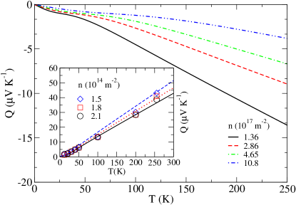
Figure 3: (Color online) Thermopower at different electronic densities $n$, in units of $10^{17}$ ${\rm{m}}^{-2}$, calculated after Eq.(38) with $v_{s}=24$ Km/s as inferred from experimental data in Ref.(Efetov and Kim (2010)). Inset: Experimental data (symbols) for hole thermopower in Ref.(Wei, Bao and Pu (2009)), compared with Eq.(38) at the corresponding hole densities (no fitting parameters besides the value of $v_{s}=24$ Km/s are used).

Therefore, we find that the thermopower at very low temperatures ($T\ll\Theta_{BG}$) becomes

$$Q(T)\sim-\frac{\pi^{2}}{3e}\frac{k_{B}^{2}T}{E_{F}}\left[1+\frac{v_{s}}{v_{F}}\frac{5!\zeta(5)}{4!\zeta(4)}\left(\frac{T}{\Theta_{BG}}\right)\right]+o(T^{3})$$ (39)

This result is in agreement with experimental data reported in the literature Wei, Bao and Pu (2009). In particular, it has been observed Wei, Bao and Pu (2009) that the thermopower in graphene depends on the carrier density as $n^{-1/2}$, and shows a linear in $T$ dependence at very low temperatures. Since the Fermi level is $E_{F}=\hbar v_{F}\sqrt{\pi n}$, it is clear that Eq.(38) obtained from our theory correctly reproduces this feature. The contribution to the total thermopower due to phonon-drag effects has been discussed in Ref.(Kubakaddi (2009)), where it is shown that it displays a $T^{3}$ dependence at low temperatures. Clearly then, the phonon drag is a negligible contribution to the total thermopower as compared to the diffusion component calculated in this work, which in agreement with the experimental data Wei, Bao and Pu (2009) reproduces the correct linear in $T$ dependence at very low temperatures.

VII Conclusions

We presented a semi-classical theory to calculate the phonon-limited transport coefficients in extrinsic graphene at high carrier densities. Our theory is based on a variational solution of the Boltzmann equation, and provides explicit analytical expressions for the various transport coefficients, such as electrical resistivity, thermal resistivity and thermopower. We showed that our analytical results are in excellent agreement with experimental data arising from two independent groups, particularly concerning the electrical resistivity Efetov and Kim (2010) and thermopower Wei, Bao and Pu (2009).

Our theoretical results suggest that, in principle, it is possible to control not only the electrical resistivity, but also the thermal resistivity and thermopower by controlling the extrinsic carrier concentration in graphene.

VIII Acknowledgements

The author wish to thank FONDECYT grant $\rm{N^{o}}$ 11100064 for financial support.

Appendix A Evaluation of angular integrals

We consider the elementary integrals over angular orientations of the wave-vectors used in the main text. Let us define the unit vector $\hat{u}=(\cos(\alpha),\sin(\alpha))$, with $\alpha$ an arbitrary (but fixed) direction along the thermal gradient or the applied electric field. As in the main text, we define the scattering angle $\theta$ by $\hat{k}\cdot\hat{k}^{\prime}=\cos(\theta)$, with $\hat{k}$, $\hat{k}^{\prime}$ the directions of the initial and final wave-vector after the electron-phonon scattering event takes place. Then, we write $\hat{k}^{\prime}=(\cos(\varphi^{\prime}),\sin(\varphi^{\prime}))$ and $\hat{k}=(\cos(\varphi^{\prime}+\theta),\sin(\varphi^{\prime}+\theta))$, respectively. Using this notation, we consider the following integrals:

$$\int_{-\pi}^{+\pi}d\varphi^{\prime}[\hat{k}\cdot\hat{u}]^{2}$$

$$=\int_{-\pi}^{+\pi}d\varphi^{\prime}\left[\cos(\alpha)\cos(\varphi^{\prime}+\theta)+\sin(\alpha)\sin(\varphi^{\prime}+\theta)\right]^{2}$$

$$=\pi[(\cos(\alpha))^{2}+(\sin(\alpha))^{2}]=\pi$$ (40)

$$\int_{-\pi}^{+\pi}d\varphi^{\prime}[\hat{k}^{\prime}\cdot\hat{u}]^{2}$$

$$=\int_{-\pi}^{+\pi}d\varphi^{\prime}\left[\cos(\alpha)\cos(\varphi^{\prime})+\sin(\alpha)\sin(\varphi^{\prime})\right]^{2}$$

$$=\pi[(\cos(\alpha))^{2}+(\sin(\alpha))^{2}]=\pi$$ (41)

$$\int_{-\pi}^{+\pi}d\varphi^{\prime}[\hat{k}\cdot\hat{u}][\hat{k}^{\prime}\cdot\hat{u}]$$

$$=\int_{-\pi}^{+\pi}d\varphi^{\prime}\left[\cos(\alpha)\cos(\varphi^{\prime}+\theta)+\sin(\alpha)\sin(\varphi^{\prime}+\theta)\right]$$

$$\times\left[\cos(\alpha)\cos(\varphi^{\prime})+\sin(\alpha)\sin(\varphi^{\prime})\right]$$

$$=\int_{-\pi}^{+\pi}d\varphi^{\prime}\left[(\cos(\alpha))^{2}\cos(\varphi^{\prime}+\theta)\cos(\varphi^{\prime})\right.$$

$$\left.+(\sin(\alpha))^{2}\sin(\varphi^{\prime}+\theta)\sin(\varphi^{\prime})+\sin(\alpha)\cos(\alpha)\right.$$

$$\left.\times\sin(2\varphi^{\prime}+\theta)\right]=\pi\cos(\theta)$$ (42)

Direct application of these basic identities leads to the following results

$$\int_{-\pi}^{+\pi}d\varphi^{\prime}[\mathbf{k}\cdot\hat{u}][\mathbf{k}^{\prime}\cdot\hat{u}]=kk^{\prime}\int_{-\pi}^{+\pi}d\varphi^{\prime}[\hat{k}\cdot\hat{u}][\hat{k}^{\prime}\cdot\hat{u}]$$

$$=\pi kk^{\prime}\cos(\theta)$$ (43)

$$\int_{-\pi}^{+\pi}d\varphi^{\prime}[\mathbf{q}\cdot\hat{u}]^{2}=\int_{-\pi}^{+\pi}d\varphi^{\prime}[(\mathbf{k}^{\prime}-\mathbf{k})\cdot\hat{u}]^{2}$$

$$=\pi(k^{2}+k^{\prime 2}-kk^{\prime}\cos(\theta))=\pi(\mathbf{k}^{\prime}-\mathbf{k})^{2}$$

$$=\pi q^{2}$$ (44)

$$\int_{-\pi}^{+\pi}d\varphi^{\prime}[\mathbf{q}\cdot\hat{u}][\mathbf{k}^{\prime}\cdot\hat{u}]=\int_{-\pi}^{+\pi}d\varphi^{\prime}[(\mathbf{k}^{\prime}-\mathbf{k})\cdot\hat{u}][\mathbf{k}^{\prime}\cdot\hat{u}]$$

$$=\pi(k^{\prime 2}-2kk^{\prime}\cos(\theta))=\pi\left(\frac{q^{2}}{2}+\frac{k^{\prime 2}-k^{2}}{2}\right)$$ (45)

Appendix B Evaluation of energy integrals at low temperature

In several calculations throughout this work, after the change of variables $x=(\epsilon-E_{F})/(k_{B}T)$ and $z=\hbar\omega/(k_{B}T)$, we use the identity

$$\int_{-\infty}^{+\infty}\frac{F(x)}{\left(1+e^{x}\right)\left(1+e^{-x-z}\right)}dx=\left(1-e^{-z}\right)^{-1}$$

$$\times\int_{-\infty}^{+\infty}\left[G(x)-G(x-z)\right]\left(-\frac{\partial f^{0}}{\partial x}\right)dx$$ (46)

with $G(x)=\int_{0}^{x}F(x^{\prime})dx^{\prime}$. This identity is straightforward to prove using integration by parts, and noting that $f^{0}(x)-f^{0}(x+z)=(1-e^{-z})(1+e^{x})^{-1}(1+e^{-x-z})^{-1}$.

The right-hand side of the equation can be further evaluated using the Sommerfeld expansion for the Fermi-Dirac distribution function at low temperatures, leading to the formula

$$\int_{-\infty}^{+\infty}\frac{F(x)}{\left(1+e^{x}\right)\left(1+e^{-x-z}\right)}dx$$

$$=(1-e^{-z})^{-1}\left\{-\int_{0}^{-z}F(x)dx+\frac{\pi^{2}}{6}[F^{{}^{\prime}}(0)-F^{{}^{\prime}}(-z)]\right\}$$

which is valid up to $o((k_{B}T/E_{F})^{4})$.

Appendix C Definition and properties of the functions $\mathcal{J}_{p}(z)$

We have defined the functions

$${\mathcal{J}}_{p}(z)=\int_{0}^{z}\frac{x^{p}\sqrt{1-(x/z)^{2}}}{(1-e^{-x})(e^{x}-1)}dx$$ (48)

The asymptotic limit of these functions, for $p>0$ an integer, is given by ${\mathcal{J}}_{p}(\infty)=p!\zeta(p)$, with $\zeta(p)$ the Riemann Zeta function. In particular, for $p=4$ and $6$ it has the values $\zeta(4)=\pi^{4}/90$ and $\zeta(6)=\pi^{6}/945$.

References

- Efetov and Kim (2010) D. K. Efetov and P. Kim, Phys. Rev. Lett. 105, 256805 (2010).
- Hwang and Das Sarma (2008) E. H. Hwang and S. Das Sarma, Phys. Rev. B 77, 115449 (2008).
- Ziman (1960) J. M. Ziman, Electrons and Phonons (University Press, 1960).
- Madelung (1978) O. Madelung, Introduction to Solid-State Theory (Springer, 1978).
- Peres and Lopes (2007) N. M. R. Peres, J. M. B. Lopes dos Santos and T. Stauber, Phys. Rev. B 76, 073412 (2007).
- Peres (2010) N. M. R. Peres, Rev. Mod. Phys. 82, 2673 (2010).
- Castro, Guinea and Peres (2009) A. H. Castro, F. Guinea, N. M. R. Peres, K. S. Novoselov and A. K. Geim, Rev. Mod. Phys. 81, 109 (2009).
- Beenakker (2008) C. W. Beenakker, Rev. Mod. Phys. 80, 1337 (2008).
- Fuhrer (2010) M. S. Fuhrer, Physics 3, 106 (2010).
- Onsager (1931) L. Onsager, Phys. Rev. 37, 405 (1931).
- Stauber, Peres and Guinea (2007) T. Stauber, N. M. R. Peres and F. Guinea, Phys. Rev. B 76, 205423 (2007).
- Munoz and Lu (2010) E. Muñoz, J. Lu and B. I. Yakobson, Nano Lett. 10, 1652 (2010).
- Saito Dresselhaus (1998) R. Saito, G. Dresselhaus and M. S. Dresselhaus Physical Properties of Carbon Nanotubes (Icp, 1998).
- Ghosh and Calizo (2008) S. Ghosh, I. Calizo, D. Teweldebrhan, E. P. Pokatilov, D. L. Nika, A. A. Balandin, W. Bao, F. Miao and C. N. Lau, Appl. Phys. Lett. 92, 151911 (2008).
- Balandin and Ghosh (2008) A. A. Balandin, S. Ghosh, I. Calizo, D. Teweldebrhan, F. Miao and C. N. Lau, Nano Lett. 8, 902 (2008).
- Wei, Bao and Pu (2009) P. Wei, W. Bao, Y. Pu, C. N. Lau and J. Shi Phys. Rev. Lett. 102, 166808 (2009).
- Kubakaddi (2009) S. S. Kubakaddi, Phys. Rev. B 79, 075417 (2009).