A Catalogue of Solar X-ray Plasma Ejections
observed by the Soft X-ray Telescope onboard YOHKOH

Abstract

A catalogue of X-ray Plasma Ejections (XPEs) observed by the Soft X-ray Telescope onboard the YOHKOH satellite has been recently developed in the Astronomical Institute of the University of Wrocław. The catalogue contains records of 368 events observed in years 1991-2001 including movies and crossreferences to associated events like flares and Coronal Mass Ejections (CMEs). 163 XPEs from 368 in the catalogue were not reported until now. A new classification scheme of XPEs is proposed in which morphology, kinematics, and recurrence are considered. The relation between individual subclasses of XPEs and the associated events was investigated. The results confirm that XPEs are strongly inhomogeneous, responding to different processes that occur in the solar corona. A subclass of erupting loop-like XPEs is a promising candidate to be a high-temperature precursor of CMEs.

1 Introduction

X-ray Plasma Ejections (XPEs) are sudden expulsions of hot magnetized plasma in the solar corona seen in X-rays. They establish a wide range of macroscopic motions showing different morphology, kinematics and physical conditions. XPEs occur usually during the impulsive phase of flares, but their connection with other solar-activity phenomena like: Coronal Mass Ejections (CMEs), prominences, radio bursts, coronal dimmings, global waves is also known. There are some restrictions in calling any motions in the corona around the flare times as XPEs. The restrictions regard the size, duration, brightness, speed, etc. and are introduced mainly by spatial, temporal and spectral resolutions of imaging instruments and their operational schemes.

XPEs have been systematically observed since 1991 when Yohkoh satellite began to operate. They became commonly known since the paper written by Shibata et al. (1995) was published. However, we note earlier articles on essentially the same phenomena from the Solar Maximum Mission (Harrison et al., 1985) and from Yohkoh (Klimchuk et al., 1994). Until now images recorded by the Yohkoh Soft X-ray Telescope, SXT (Tsuneta et al., 1991) are the largest database of XPEs, even though the newer solar X-ray imaging instruments operate, e.g., GOES Solar X-ray Imager, Reuven Ramaty High-Energy Solar Spectroscopic Imager (RHESSI), Hinode X-Ray Telescope.

Detailed analyses of individual XPEs were performed first by Tsuneta (1997) and Ohyama & Shibata (1997, 1998). In these papers the authors determined values of physical parameters describing an XPE using temperature and emission measure maps obtained from SXT images. The maps allowed them to investigate overall magnetic configuration including a flare loop and a reconnection region. They also used hard X-ray light curves, derived by the Yohkoh Hard X-ray Telescope, HXT (Kosugi et al., 1991), for a detailed description of reconnection timing.

Nitta & Akiyama (1999) made the first attempt to correlate XPEs and CMEs. For 17 well-observed limb flares they found that flares associated with CMEs show XPEs and opposite – flares not associated with CMEs also lack XPEs. A more extensive investigation of association between XPEs and flares was performed by Ohyama & Shibata (2000). For 57 well-observed limb flares they found that almost 70% show XPEs. They also reported dependence on X-ray class, namely the association is larger for stronger flares, but it could be caused by observational biases.

To investigate interesting examples of XPEs other Yohkoh instruments also have been used, namely the HXT (Hudson et al., 2001) and the Bragg Crystal Spectrometer, BCS (Tomczak, 2005). In both papers a special location of investigated events has been chosen. These XPEs occurred far behind the solar limb and due to their fast expansion they came into the view of an instrument before brighter flares, which expand slower. It is virtually the only way for using full-Sun instruments like the BCS to resolve faint soft X-ray emission of XPEs. The behind-the-limb location also protects against strong emission of footpoint hard X-ray sources of flares, which usually dominate fainter coronal emission. The obtained results proved that an XPE can conatin energetic non-thermal electrons (Hudson et al., 2001) and superhot thermal plasma (Tomczak, 2005).

An important progress in investigation of XPEs gave a trilogy made by Kim et al. (2004, 2005a, 2005b). They investigated systematically SXT observations obtained during a two-year interval and found 137 XPEs. The events were a subject of multipurpose analysis – the authors introduced a morphological classification of XPEs, investigated their kinematics, specified the association with flares and CMEs. The present name of XPEs also comes from these papers. We recapitulate the results of Kim et al. in details in further sections, where we compare them to our results.

More recently, an association between XPEs and radio events and prominences has been investigated. In statistical surveys Shanmugaraju et al. (2006) studied type II radio bursts, whereas Kołoma$\acute{\rm{n}}$ski et al. (2007) studied drifting pulsating structures (DPS). Both surveys suggest a kind of connection between XPEs and radio events but further examinations are needed to establish the connection. The relationship between hot (XPEs) and cold (prominences) ejections was discussed by Ohyama & Shibata (2008); Kim et al. (2009) for single events, which was followed up with statistical studies (Chmielewska & Tomczak, 2012).

Finally, in our short review illustrating a research progress we would like to recall the two following papers. Firstly, the results of a quantitative analysis of SXT images describing time evolution of basic physical parameters for 12 XPEs were given by Tomczak & Ronowicz (2007). Secondly, after extensive analysis of a complex XPE that consisted of several recurrent episodes, Nishizuka et al. (2010) reported a close connection between sequential ejections and successive hard X-ray bursts.

The most commonly accepted physical explanation of XPEs connects these phenomena directly with flare magnetic reconnection. Shibata et al. (1995) regarded XPEs as a proof of the presence of plasmoids driven by magnetic reconnection occurring above a soft X-ray loop in short-duration, compact-loop flares similar to the canonical 2D CSHKP model ($\check{\rm{S}}$vestka & Cliver, 1992, and references therein), which was proposed for long-term, two-ribbon flares. In this way, Shibata et al. (1995) postulated a unification of two observationally distinct classes of flares, i.e. two-ribbon flares and compact-loop flares, by a single mechanism of magnetic reconnection called the plasmoid-induced-reconnection model.

The first qualitative studies of individual events (Ohyama & Shibata, 1997, 1998) reported that the measured velocities of XPEs are much smaller than the velocity of reconnection outflow expected from the model to be about the Alfv$\rm{\acute{e}}$n speed. To reconcile this discrepancy the authors suggested: (1) the high density of the XPEs, (2) the time evolution effect (i.e., the plasmoid should be accelerated as it propagates, thus the investigated XPEs have not yet reached the maximum velocity), or (3) an interaction with coronal magnetic fields overlying the XPEs.

Although more recently, 2D resistive-MHD numerical simulations of the reconnection explain kinematical properties of various observational features attributed to the current-sheet plasmoids (B$\acute{\rm{a}}$rta, Vr$\check{\rm{s}}$nak & Karlick$\acute{\rm{y}}$, 2008), it has been expected that 3D reconnection renders a more realistic description of eruptive phenomena. For example, Nitta, Freeland & Liu (2010) suggested 3D quadrupolar reconnection of two loop systems that appear to exchange their footpoints as a result of loop-loop interaction (Aschwanden et al., 1999).

On the other hand, in some cases the XPEs seem to play the same role as phenomena called precursors of CMEs (Cheng et al., 2011). This opinion is supported observationally by common kinematical evolution of XPEs and CMEs (Gallagher, Lawrence & Dennis, 2003; Dauphin, Vilmer & Krucker, 2006; Bak-Ste$\acute{\rm{s}}$licka, Kołoma$\acute{\rm{n}}$ski & Mrozek, 2011) as well as their morphological resemblance (Kim et al., 2005a). If so, loss of equilibrium or MHD instability, commonly accepted as one of the CME triggering mechanism (Forbes, 2000), also should be taken seriously into consideration as a cause of XPEs.

Reports concerning XPE observations in the SXT database were scattered until now across many different sources: refereed articles, conference communications, electronic bulletins, etc. An exception was the survey given by Kim et al. (2005a), which includes almost all the XPEs associated with limb flares for a two-years interval. Our motivation was to ingest all available reports in one catalogue and organize them in a uniform way for an easy usage. We have examined SXT images in those time intervals, in which any systematic searches of XPEs did not perform.

Knowledge about XPEs has so far been shaped by a limited number of events that have repeatedly appeared in the literature. Our catalogue is meant to serve as a convenient tool for every scientist who wants to better understand the nature of XPEs.

2 Description of the catalogue

2.1 General contents

The catalogue contains the all XPEs we know that were observed by the SXT during the entire Yohkoh operations, i.e. between 1991 October 1 and 2001 December 14. There are three main surveys of events that we used in our catalogue:

1. Kim et al. (2005a), which contains 137 limb events, observed between 1999 April and 2001 March.

2. Ohyama (2009, private communication) with 53 limb events that occurred between 1991 October and 1998 August. The survey was prepared for the aim of statistical research (Ohyama & Shibata, 2000), but it was not published.

3. Chmielewska (2010), which reports 113 events, observed basically within two time intervals: 1998 September – 1999 March and 2001 April – 2001 December that were not systematically searched before.

We also incorporated 65 XPEs reported in other scientific papers as well as in the electronic bulletin YOHKOH SXT Science Nuggets.

Keeping in mind the examination of SXT images made by different authors, we can conclude that the list of XPEs associated with limb flares (defined as $|\lambda|>60^{\circ}$, where $\lambda$ is heliographic longitude) is almost complete. On the other hand, the list of XPEs associated with disk flares is largely incomplete, with the exception of time intervals examined by Chmielewska (2010). Occasional reports of XPEs not associated with any flares (Klimchuk et al., 1994) teach us that the SXT images made without any flares should be also examined and this work still awaits to be done.

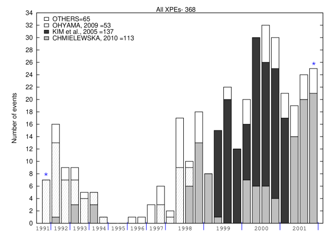
Figure 1: Frequency of XPEs for each year during the Yohkoh mission. Bin sizes are 6 and 3 months for years 1991-1997 and 1998-2001, respectively. The bins marked with stars refer to partial years. Each survey mentioned in Section 3.1 is indicated differently.

In summary, our catalogue contains 368 events. Time frequency of XPEs occurrence during the Yohkoh mission is given in Fig. 1, where sizes of bins are 6 or 3 months for years 1991-1997 and 1998-2001, respectively. This traces variability of general solar activity. A larger occurrence rate in cycle 23 in comparison with cycle 22 may be attributable to the revision of the SXT flare mode observing sequences. Indeed, the ratio of the number of XPEs and that of flares taken from the Solar-Geophysical Data (SGD) is 3.6 times greater for solar cycle 23 than for cycle 22.

Before 1997, a routine scheme of observations during the flare mode was dominated by images in which the exposure time and the position of the field of view (typically 2.5$\times$2.5 arcmin²) were automatically adjusted by the signals and locations of the brightest pixels. XPEs are distinctly fainter and located higher in the corona than flares. Thus, they had usually too poor statistics during short exposure times and due to a fast expansion they left immediately the narrow field of view. Under these circumstances, XPEs were rarely well-observed.

In 1997, the frequency of images with sufficiently long and constant exposures and broader field-of-view (5.2 $\times$ 5.2 arcmin² and 10.5 $\times$ 10.5 arcmin²) was increased to every 10-20 s (Nitta & Akiyama, 1999). This observational scheme worked more favorably for the XPEs identification, however flare structures seen in those images often suffer from heavy saturation that manifests itself as vertical spikes disturbing a picture of XPEs.

We registered events to the catalogue on the basis of the SXT observations exclusively. For this reason, we omitted some X-ray ejections from years 1991-2001 identified using observations made with other instruments alone, like the HXT, e.g. Hudson et al. (2001).

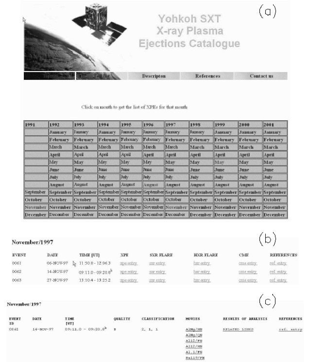
Figure 2: Overview of the Yohkoh SXT XPE Catalogue, which resides online at http://www.astro.uni.wroc.pl/XPE/catalogue.html. (a) The main entry into the catalogue as a matrix of years and months of observations. (b) A few of the entries in the catalogue for 1997 November. (c) A screenshot for the XPE entry of event No. 62 on 1997 November 14.

The online catalogue resides at http://www.astro.uni.wroc.pl/XPE/catalogue.html since 2010 October 22. It is also linked from the Yohkoh Legacy Data Archive (Takeda et al., 2009). The general arrangement of the catalogue as a matrix of years and months of observation is presented in Fig. 2a. After clicking the month, each XPE is identified by a chronological catalogue number, date, and time of occurrence. The letter (a) added to a start time means that the XPE began earlier than shown in the available movies. The letter (b) added to an end time means that the XPE finished later than shown in the available movies. The letter (c) added to an end time means a time interval of available movies in which we cannot identify the XPE reported earlier by other authors. Each events has links to five entries that provide detailed information on the XPE, flare (SXR and HXR), CME, and references on the XPE (see an example in Fig. 2b).

2.2 The “XPE” entry

This entry contains 8 columns labeled as follows: (1) event ID, (2) date, (3) time, (4) quality, (5) classification, (6) movies, (7) results of analysis, and (8) references (see an example in (Fig. 2c). The first three columns are replicated from the higher entry.

In Col. (4), we indicate the quality of available SXT observations by assigning one letter between (A) and (D). The letter (A) means the highest quality: an XPE is clearly seen and only slightly disturbed by flare saturation, observations have almost full spatial and time coverage, images are made by at least two different filters. In conclusion, events with this letter are a good source for any kind of quantitative analysis including plasma diagnostics on the basis of the filter-ratio method (Hara et al., 1992). The letter (B) also means quite good quality of observations, but the usage of only a one filter in some cases makes a plasma diagnostics unavailable. Nevertheless, XPEs marked with this letter are always good for kinematical studies. The letter (C) means poor quality for some of the following reasons: the brightness of the XPE only marginally above the background, short observation window, inadequate field-of-view, or strong effect from flare saturation. For events with this letter only limited analyses are usually possible, e.g. a description with our 3-parameters classification. The letter (D) is designed for XPEs, which were mentioned by other authors but whose presence is not confirmed in the movies that we made.

In Col. (5) we characterize general observational features of XPEs using a new classification scheme that we have developed in this catalogue. In our classification we define three criteria considering: (a) morphology of an XPE, (b) its kinematics, and (c) recurrence. Examining each criterion we distinguish two subclasses of events only: (a) 1 – collimated, 2 – loop-like; (b) 1 – confined, 2 – eruptive; (c) 1 – single, 2 – recurrent. In consequence, our classification can resolve $2^{3}=8$ subclasses.

Our motivation should be commented in the context of the earlier classification made by Kim et al. (2004), who proposed 5 morphological groups of XPEs: a loop-type, spray-type, jet-type, confined, and other. In our opinion, the classification that is too ‘hair-splitting’ may be uncomfortable in practical usage because it is easy to make a wrong assignment in case of poor quality of the observational data or their limited coverage. We may recall attempts of organizing properties of CMEs as observed by different coronagraphs (Munro & Sime, 1985; Howard et al., 1985; Burkepile & St. Cyr, 1993; Gopalswamy et al., 2009). They have never worked out any commonly accepted classification scheme for CMEs on the basis of morphological features only.

Our morphological criterion resolves only a direction of soft X-ray plasma movement in comparison with the direction of local magnetic field. Roughly speaking, in the case of the subclass 1 the direction is parallel i.e. along the already existing magnetic field lines, in the case of the subclass 2 — perpendicular i.e. across the already existing lines (or strictly speaking – together with them). XPEs from the first morphological subclass usually take a form of a blob or a column of matter propagating within a bundle of magnetic lines without any serious modification of their structure. Therefore, these events are more collimated (hence its name) and less energetic. A direction of their motions depends on the configuration of guiding lines. Our subclass 1 comprises the majority of events classified by Kim et al. (2004) as the spray-type and jet-type events. XPEs from the second morphological subclass take a form of a rising loop or a system of loops. Our subclass 2 is very similar to the loop-type events proposed by Kim et al. (2004). Some events showed features of both morphological subclasses, 1 and 2, in this case we classified them according to a more evident feature.

For the XPE assignment into one of the kinematical subclasses we have chosen height increase rate above the chromosphere, $\dot{h}$. A negative value, $\dot{h}<0$, means the subclass 1, the opposite case, $\dot{h}\geq 0$ means the subclass 2. There are several papers presenting plots $h(t)$ for events belonging to both subclasses (Klimchuk et al., 1994; Tsuneta, 1997; Ohyama & Shibata, 1997, 1998; Nitta & Akiyama, 1999; Kundu et al., 2001; Alexander, Metcalf & Nitta, 2002; Tomczak, 2003, 2004; Kim et al., 2005a, b; Ohyama & Shibata, 2008; Kim et al., 2009; Nishizuka et al., 2010). XPEs from the first kinematical subclass can be connected with plasma motion within closed magnetic structures as well as with some changes in a plasma situation or in the local magnetic field structure which do not evacuate any mass from the Sun. In summary, XPEs from the first kinematical subclass suggest the presence of kind of magnetic or gravitational confinement of X-ray plasma. For XPEs from the second kinematical subclass, an increasing velocity in the radial direction in the field of view of the SXT allows us to anticipate further expansion leading to irreversible changes (eruption) of the local magnetic field. In consequence, at least a part of the plasma escapes from the Sun.

For many weak XPEs a construction of the diagram $h$ vs. $t$ was impossible. Therefore, we estimated $dh/dt$ qualitatively by watching the expansion rate of XPEs in movies made with images uniformly spaced in time. In some cases the classification was problematic because of a limited coverage of available observations, hence we added a question mark to the digit for this criterion.

According to our third criterion we separate disposable, unique XPEs that occurred once in a time (subclass 1) from recurrent events for which following expanding structures can be seen with time (subclass 2). The majority of XPEs described in the literature belongs to the subclass 1, however samples of the subclass 2 were already presented (Nitta & Akiyama, 1999; Tomczak, 2003; Nishizuka et al., 2010). A partial time coverage of the available observations probably introduces a bias toward single XPEs, because a narrow observational window allows us to resolve only a single feature even for recurrent XPEs.

Especially important is Col. (6) in which all available movies illustrating evolution of the XPE are collected. The movies consist of images obtained by the SXT and are written in the MPEG format. Images made by using particular filters and spatial resolutions are collected in separate movies. We label the movies to indicate their contents, e.g., AlMg/HN marks images obtained with the AlMg filter of half resolution. We use the following standard annotations of filters and spatial resolutions applied in the Yohkoh software (Morrison, 1994): the filter Al.1 – the wavelength range 2.5-36 Å , AlMg – 2.4-32 Å , Mg3 – 2.4-23 Å , Al12 – 2.4-13 Å , Be119 – 2.3-10 Å ; the full resolution, FN, – 2.45 arcsec, half resolution, HN, – 4.9 arcsec, quarter resolution, QN, – 9.8 arcsec. A particular resolution means a specific field of view: 2.6 $\times$ 2.6 arcmin², 5.2 $\times$ 5.2 arcmin², 10.5 $\times$ 10.5 arcmin², for the FN, HN, and QN resolution, respectively. Sometimes we divided images made with the same filter and the same spatial resolution onto separate movies consisting of images made with the same time exposition. In that case, the labels contain additionally successive roman digits.

The movies consist of images that we previously processed using the standard Yohkoh routine SXT_PREP, allowing us to reduce an influence of typical instrumental biases, e.g. telemetry compression, electronic offset, dark current, straylight, de-jittering. In the images the heliospheric coordinates are overwritten by using the SolarSoft routine PLOT_MAP. For better identification of a faint features slightly above the background, we represented a signal distribution with non-linear color tables Nos. 16 (“Haze”), 33 (“Blue-red”), or 3 (“Red temperature”) available in the Interactive Data Language (IDL). Images that form movies in the catalogue are sometimes non-uniformly spaced in time, therefore it is strongly recommended to watch a time print that is present in each image.

The XPEs for which a more detailed analysis have been already performed show in Col. (7) an entry with a concise report concerning results. Inside the report, the obtained values of investigated parameters like velocity, acceleration, temperature, emission measure, electron density, pressure, and secondaries, as well as references, are given. For 14 events (Nos. 29, 30, 34, 53, 62, 67, 72, 126, 144, 169, 252, 293, 303, and 330) a more complete set of results is presented in form of plots and tables illustrating the whole evolution (Ronowicz, 2007).

Finally, in Col. (8) references to all the reports (also in the electronic form) in the chronological order are given.

2.3 Other catalogue entries

The “SXR Flare” entry contains a basic info about a flare that was associated with the given XPE. Finding the associated flare for the majority of XPEs in the catalogue was very easy. A flare is seen usually in movies illustrating evolution of an XPE as heavy saturation due to its much stronger soft X-ray radiation. In several cases a flare occurred simultaneously with an XPE but in another active region. We considered this flare as the associated event only when some distinct magnetic loops connecting both active regions were seen. Finally, there are several XPEs that occurred when no flare was observed on the Sun.

Each record describes the following attributes: date, time of start, maximum, and end defined on the basis of the Geostationary Operational Environmental Satellites (GOES) 1–8 Å light curve, GOES class, location in heliographic coordinates, NOAA active region number. By clicking on the GOES class, one can view the GOES light curves in two wavelength ranges: 1–8 Å (upper) and 0.5–4 Å (lower). Time span of plots is always two hours and includes the occurrence of an XPE, which is marked by vertical lines. The hatched area on the plot represents Yohkoh nights.

Records presented in this entry are generally adopted from the SGD, however some clarifications and supplements were necessary. For example, the lacking locations were completed on the basis of SXT images as a place of flare bright loop-top kernels. The values obtained in this way are given in parenthesis. Coordinates of events that occurred behind the solar limb are taken basically from Tomczak (2009).

If no flare was associated with an XPE, the tags devoted to flare characteristics are empty. Exceptions are GOES light curves, heliographic coordinates, and NOAA active region number. The last two tags describe then an XPE.

The “HXR Flare” entry presents some attributes of hard X-rays emitted by a flare that was associated with a given XPE. We used data from the HXT onboard Yohkoh. This telescope measured the hard X-ray flux in four energy bands: 14-23 (L), 23-33 (M1), 33-53 (M2), and 53-93 keV (H). Each record contains peak time and peak count rate (together with the background), inferred for the energy band M1. By clicking on the peak count rate, one can view the HXT light curves in all energy bands. Time span of plots usually includes the maximum of hard X-ray flux and the occurrence of an XPE, which is marked by vertical lines. Wherever available, we also include the event ID from the Yohkoh Flare Catalogue (HXT/SXT/SXS/HXS)

If no flare was associated with an XPE, the tags devoted to flare characteristics are empty. In case the hard X-ray flux in the energy band M1 was below the doubled value of the background we left the tags describing peak time and peak time rate empty.

The “CME” entry contains some attributes of a CME that was associated with a given XPE. The observations are derived by the Large Angle and Spectrometric Coronagraph (LASCO) onboard the Solar and Heliospheric Observatory (SOHO). From the SOHO LASCO CME Catalog (Gopalswamy et al., 2009) values of the following parameters are given: date and time of the first appearance in the C2 coronagraph field of view, central position angle, angular width, speed from linear fit to the $h(t)$ measurements, acceleration inferred from the quadratic fit. The first appearance time is the link to the beginning of the list of events in the SOHO LASCO CME Catalog for a given year and month. By clicking on the entry “Related links” one can view a javascipt movie of the CMEs within the C2 field of view for a given day. Movies reside at the the homepage of the SOHO LASCO CME Catalog.

According to Yashiro et al. (2008), we consider a pair XPE-CME as physically connected if the XPE occurred within position angles defined by the CME angular width increased by 10^∘ from both sides. Moreover, time of the XPE occurrence had to fall within 3-hours-interval centered around extrapolated time of the CME start for $h=1R_{\sun}$. For extrapolation we used time of the first appearance in the LASCO/C2 field of view and linear velocity taken from the SOHO LASCO CME Catalog. The “CME” entry is empty when the XPE occurred during a LASCO gap. XPEs not associated with a CME are labeled: ’No related event’.

In “References” entry the references to all reports (also in the electronic form), known for us, that mentioned a particular XPE are given in the chronological order.

2.4 Statistics of the catalogue content

Some useful characteristics of XPEs included in the catalogue are extracted in Table A Catalogue of Solar X-ray Plasma Ejections observed by the Soft X-ray Telescope onboard YOHKOH. In this subsection we discuss general statistics of the catalogue content.

In Table 2 the quality of XPE observations from the catalogue is summarized. The most frequent are events that we categorized as (B) and (C). Contribution of remaining categories is marginal. In Sections 3 and 4 we present results of a statistical analysis that was performed for two different populations of events: from (A) to (C) and from (A) to (B). The first population is more frequent, which offers some advantages in statistical approach, however for events categorized as (C) observations are often not complete enough to give confidence in our classification choices. In consequence, in the first population an additional bias can be introduced which is inadvisable. We expect that this problem is overcome for less frequent, second population of XPEs which was better observed.

In Table 3 we summarize heliographic longitudes of XPEs in the catalogue. A distinct concentration of the XPEs around the solar limb is seen. This is an artificial effect caused by observational constrains. XPEs are easier for detection when we observe them against the dark background sky than when we observe them between plenty of different features seen on the solar disk. Moreover, in two from three main surveys that we used in our catalogue (Kim et al., 2005a, Ohyama 2009, private communication), only flares that occurred close to the solar limb ($|\lambda|>60^{\circ}$) were systematically reviewed.

Is it possible to estimate the actual number of XPEs, which occurred on the Sun during the Yohkoh years? Assuming their uniform distribution with heliographic longitude and taking the number for the interval $60^{\circ}\leq|\lambda|\leq 90^{\circ}$ as the most representative, we obtain a value $6\times 218\approx 1300$. Including a duty time of Yohkoh to be about 0.65 (ratio of satellite day to the total orbital period) we obtain a number $2\times 10^{3}$.

However, even this huge number could be significantly lower than actual due to several reasons. Firstly, we do not include an influence of worse detection conditions before 1997. Secondly, for strong flares, especially in 2001, the conditions for detecting XPEs were quite bad because of too long exposures. Thirdly, the estimated number is roughly representative for flares stronger than the GOES class C5-C6. Only for those events the flare mode was initiated in the Yohkoh operation (Tsuneta et al., 1991) and this mode guarantees a sufficient time resolution of an image cadence for a successful detection of XPEs. XPEs associated with weaker flares are only known accidentally, since no systematic examination of images recorded during the quiet mode of the Yohkoh satellite has been performed yet.

In conclusion, XPEs should be considered as very frequent events occurring in the solar corona. XPEs described in the catalogue are only a minor representation of a countless population of events, which are typical for the hot solar corona.

In Table 4 we present a time coverage of the observed XPEs. Evolution of an important fraction of events (42.6%) is illustrated only partially. This limits its detailed investigation. Even relatively simple activities like classification can be meaningless. For example, XPEs classified as single and observed only partially can be actually recurrent.

In Table 5 we present a number of XPEs that were classified onto one of eight subclasses defined under following three criteria: morphological, kinematical, and recurrence. We organize the results twofold: for the total population and for carefully selected events. In the second case we omitted events categorized as (C), untrustworthy assignments of kinematical criterion as shown in the catalogue with the question mark, and examples classified as single in case of partial time-coverage of observations. It reduces the whole population almost three times and for particular subclasses even more, but we believe that numbers less affected by observational limits, seen in the last column of Table 5, are more representative for real conditions.

What do these numbers tell us about XPEs? At first sight, loop-like XPEs seem to be more frequent than collimated XPEs of a factor 2.1 or 3.2 for total population and special selection, respectively. However, it can be caused by the effect of observational selection. On average, loop-like XPEs are more massive than collimated ones (Tomczak & Ronowicz, 2007), thus they are easier for detection above the background. Indeed, the exclusion of faint events categorized as (C) increases relative contribution of loop-like XPEs. It is interesting that in Kim et al. (2005a) the number of loop-type XPEs (60) only slightly outnumbers the sum of spray-type and jet-type events (51).

For other relations, the carefully selected events seem to be less affected by observational constraints than those of the entire populations. Therefore we conclude that the former events adequately characterize intrinsic features of particular subclasses. For example, for loop-like XPEs the relation between eruptive and confined or between recurrent and single events is distinctly different from that for collimated XPEs. Loop-like XPEs are dominantly eruptive (82 to 14) and recurrent (59 to 37), whereas collimated XPEs are more frequently confined (19 to 11) and single (20 to 10).

We would like to stress that subclasses of XPEs defined by us resemble some types of classical prominences observed in H$\alpha$ line (Tandberg-Hanssen, 1995). Namely, a surge is a prominence that is collimated and confined, a spray is a prominence that is collimated and eruptive, a loop-like and confined event we call as an activation of a prominence, and a loop-like and eruptive event is an eruptive prominence or ’disparision brisque’. Classifications of prominences do not distinguish the recurrence criterion, nevertheless there are known observations, in which aforementioned types of prominences were observed as single or recurrent events (Rompolt 2011, private communication). This similarity between XPEs and prominences suggests a close association between hot and cold components of active regions. This relation was not investigated in details so far, except for Ohyama & Shibata (2008).

3 XPEs association with solar flare

Using the classification we were able to separate several subclasses of XPEs looking more homogeneous than the full population. Unfortunately, we are not sure if particular subclasses of XPEs refer to events that are physically different. A quantitative analysis of soft X-ray images would give closer confirmation, however for the majority of XPEs in the catalogue this kind of analysis is practically unreliable, due to minor signal and other observational limits. Therefore, the main motivation of this section is to justify the presence of physically different subclasses of XPEs by a comparison of properties of other solar-activity phenomena associated with particular XPEs. Basic characteristics of flares and CMEs are known well. In this Section we present the association of XPEs with flares, in Section 4 we present the association of XPEs with CMEs.

3.1 Soft X-rays

It has been commonly agreed that an XPE is a consequence of a flare occurrence. As a matter of fact, there are 5 XPEs in our catalogue, for which we could not find any associated flare. However, this sample is too small to justify the existence of flareless XPEs. Moreover, three of the five XPEs occurred close enough to the solar limb that they might have come from flares from the backside. Are they just the tip of an iceberg? The answer may depend on extensive and careful examination of SXT images made in the quiet mode.

3.1.1 Time coincidence

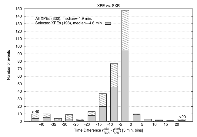
Figure 3: Histogram of time differences between the SXR start of the associated flare (from GOES light curve) and the XPE start. Gray and hatched bins represent the better observed XPEs (quality A-B, so-called selected XPEs) and the rest of XPEs (quality C), respectively. The size of bins is 5 minutes with exception of outermost ones. Numbers of all the considered XPEs and the selected XPEs as well as their medians are given.

For better insight in time coincidence between XPEs and flares we mark the time of an XPE on the GOES light curve of an associated flare. In Fig. 3 we present a histogram of time differences between start times of flares and XPEs for 330 pairs of events. In 311 cases from 330 (94.2%), an increase of soft X-ray emission occurred earlier than the XPE. The time difference is very often several minutes only (see maximum and median of the histogram), however higher values also occur. Similar conclusions can be given regarding better observed XPEs of quality A and B (compare the gray bins in Fig. 3). Similar histograms made for particular subclasses of the XPEs introduced in our classification do not show any important differences.

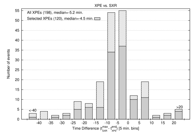
Figure 4: Histogram of time differences between the SXR maximum of the associated flare (from GOES light curve) and the XPE end. Gray and hatched bins represent the better observed XPEs (quality A-B, so-called selected XPEs) and the rest of XPEs (quality C), respectively. The size of bins is 5 minutes with exception of outermost ones. Numbers of all the considered XPEs and the selected XPEs as well as their medians are given.

In Fig. 4 we present a histogram of time differences between the end of XPEs and the peak of the associated flares as determined from the GOES light curves. In about 20% of investigated samples (41 from 198) any XPEs were completed before the flare peak, i.e. within the rising phase of a flare. For almost 80% of events the final evolution of XPEs is seen after the maximum of soft X-ray emission, very often no longer than 10 minutes (108 examples from 198, 54.5%). Similar conclusions can be given regarding better observed XPEs of quality A and B (compare the gray bins in Fig. 4). Similar histograms made for particular subclasses of XPEs introduced in our classification do not show any important differences.

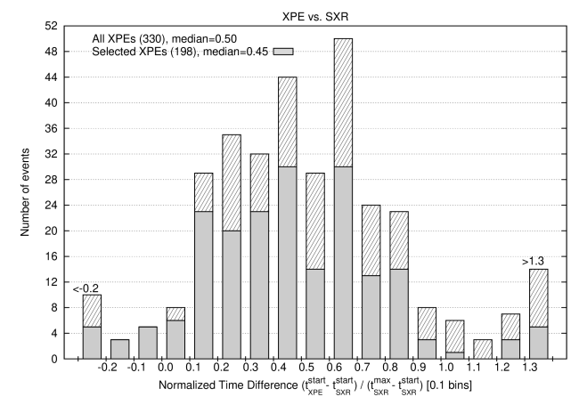
Figure 5: Histogram of time differences between the SXR start of the associated flare (from GOES light curve) and the XPE start normalized with the flare rising-phase duration. Gray and hatched bins represent the better observed XPEs (quality A-B, so-called selected XPEs) and the rest of XPEs (quality C), respectively. The size of bins is 0.1 of the flare rising-phase duration with exception of outermost ones. Numbers of all the considered XPEs and the selected XPEs as well as their medians are given.

The above results should be normalized to the time scales of flares. Therefore, we have prepared counterparts of Figs. 3 and 4 in which we normalize time differences with the flare rising-phase duration. In Fig. 5 we illustrate occurrences of the XPE start: negative values mean that a XPE preceded its flare, the value 0 – simultaneous start, the value 1 – start of a XPE at the maximum of its flare, values grater than 1 – later XPE start. As we see, the majority of XPEs (282 from 330, 85.5%) starts within the rising phase of flares. This rule is fulfilled even stronger for better observed XPEs (gray bins) – 176 from 198, 88.8%.

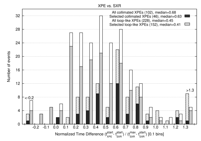
Figure 6: Histogram of time differences between the SXR start of the associated flare (from GOES light curve) and the XPE start normalized with the flare rising-phase duration made for collimated and loop-like XPEs separately. Black or gray and hatched or white bins represent the better observed XPEs (quality A-B, so-called selected XPEs) and the rest of XPEs (quality C), respectively. The size of bins is 0.1 of the flare rising-phase duration with exception of outermost ones. Numbers of all the considered XPEs and the selected XPEs as well as their medians are given.

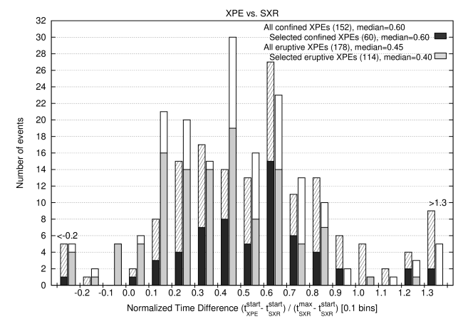
Figure 7: Histogram of time differences between the SXR start of the associated flare (from GOES light curve) and the XPE start normalized with the flare rising-phase duration made for confined and eruptive XPEs separately. Black or gray and hatched or white bins represent the better observed XPEs (quality A-B, so-called selected XPEs) and the rest of XPEs (quality C), respectively. The size of bins is 0.1 of the flare rising-phase duration with exception of outermost ones. Numbers of all the considered XPEs and the selected XPEs as well as their medians are given.

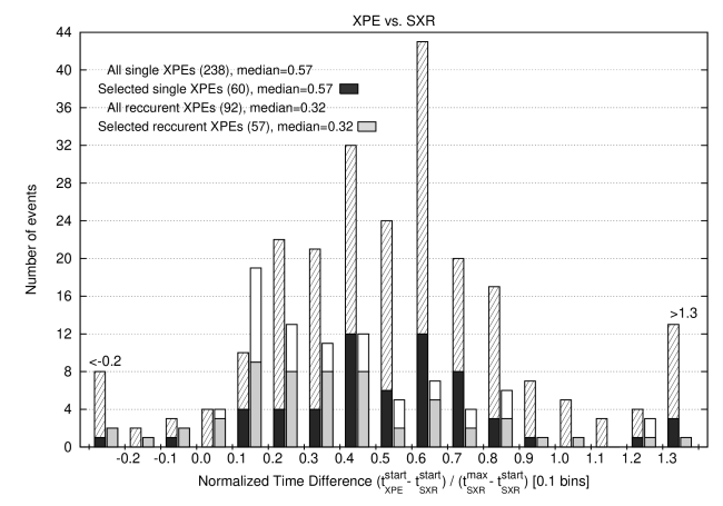
Figure 8: Histogram of time differences between the SXR start of the associated flare (from GOES light curve) and the XPE start normalized with the flare rising-phase duration made for single and recurrent XPEs separately. Black or gray and hatched or white bins represent the better XPEs (quality A-B, so-called selected XPEs) and the rest of XPEs (quality C), respectively. The size of bins is 0.1 of the flare rising-phase duration with exception of outermost ones. Numbers of all the considered XPEs and the selected XPEs as well as their medians are given.

Interesting results are revealed by further versions of Fig. 5, in which particular subclasses of XPEs are separated: collimated and loop-like, confined and eruptive, single and recurrent, in Figs. 6-8, respectively. In these figures, we show side-by-side the distributions of the XPEs that have contrasting properties. For example, in Fig. 6 loop-like XPEs show tendency to start earlier in the rising phase of flares than collimated ones: the difference for medians is more than 0.2 of the rising-phase duration. A similar tendency is seen in Fig. 7 where eruptive XPEs start earlier in the rising phase of associated flares than confined ones and in Fig. 8 where recurrent XPEs precede, on average, single ones.

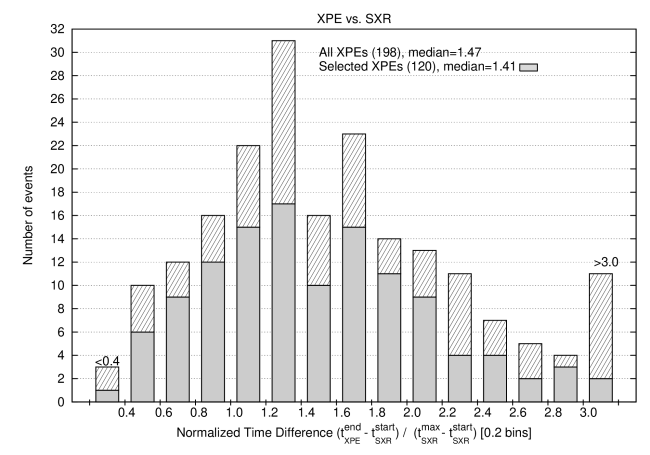
Figure 9: Histogram of time differences between the SXR start of the associated flare (from GOES light curve) and the XPE end normalized with the flare rising-phase duration. Gray and hatched bins represent the better observed XPEs (quality A-B, so-called selected XPEs) and the rest of XPEs (quality C), respectively. The size of bins is 0.2 of the flare rising-phase duration with exception of outermost ones. Numbers of all the considered XPEs and the selected XPEs as well as their medians are given.

In Fig. 9 we have normalized time differences between the XPE end and the associated flare start with the rising-phase duration of a flare. In this scale the value 1 means that the XPE end occurred exactly at the maximum of the associated flare. The histogram is rather gradual with two maxima between 1.2-1.4 and 1.6-1.8. The number of XPEs lower than the first maximum and greater than the second one decreases systematically with a marginal contribution of those that are lower than 0.4 and greater than 3. It means that all soft X-ray plasma motions are limited within a relatively narrow part of total duration of associated flares.

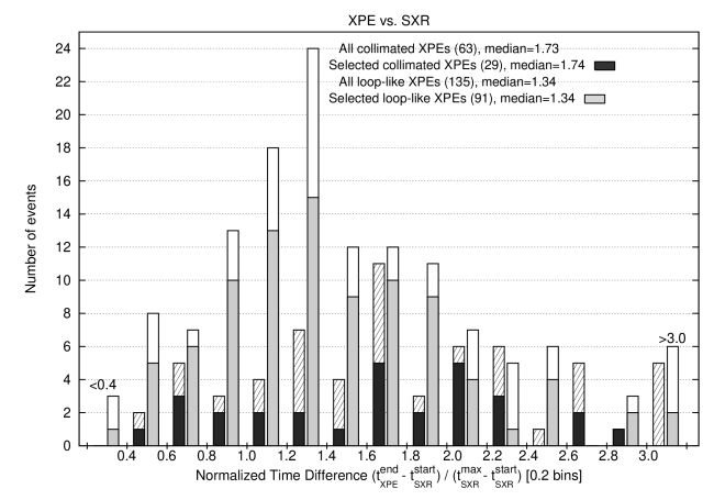
Figure 10: Histogram of time differences between the SXR start of the associated flare (from GOES light curve) and the XPE end normalized with the flare rising-phase duration made for collimated and loop-like XPEs separately. Black or gray and hatched or white bins represent the better observed XPEs (quality A-B, so-called selected XPEs) and the rest of XPEs (quality C), respectively. The size of bins is 0.2 of the flare rising-phase duration with exception of outermost ones. Numbers of all the considered XPEs and the selected XPEs as well as their medians are given.

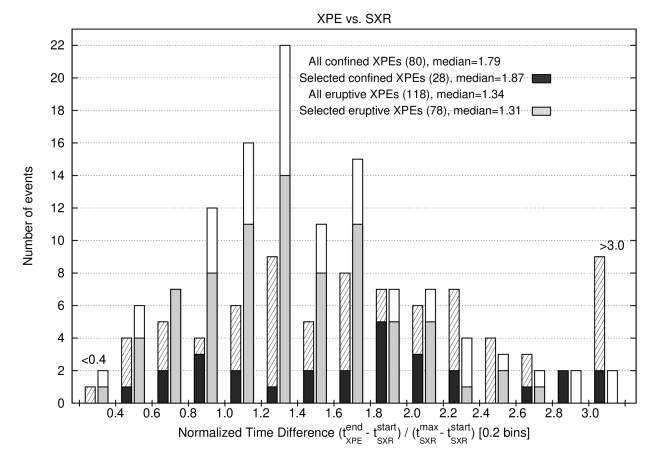
Figure 11: Histogram of time differences between the SXR start of the associated flare (from GOES light curve) and the XPE end normalized with the flare rising-phase duration made for confined and eruptive XPEs separately. Black or gray and hatched or white bins represent the better observed XPEs (quality A-B, so-called selected XPEs) and the rest of XPEs (quality C), respectively. The size of bins is 0.2 of the flare rising-phase duration with exception of outermost ones. Numbers of all the considered XPEs and the selected XPEs as well as their medians are given.

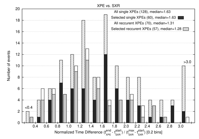
Figure 12: Histogram of time differences between the SXR start of the associated flare (from GOES light curve) and the XPE end normalized with the flare rising-phase duration made for single and recurrent XPEs separately. Black or gray and hatched or white bins represent the better observed XPEs (quality A-B, so-called selected XPEs) and the rest of XPEs (quality C), respectively. The size of bins is 0.2 of the flare rising-phase duration with exception of outermost ones. Numbers of all the considered XPEs and the selected XPEs as well as their medians are given.

The variants of Fig. 9, in which particular subclasses of XPEs are separated: collimated and loop-like, confined and eruptive, single and recurrent, are presented in Figs. 10-12, respectively. In these figures, as in Figs. 6-8, we show side-by-side the distributions of the XPEs that have contrasting properties. In Fig. 10 the collimated XPEs seems to last longer, on average, than the loop-like ones: medians of both distribution differ by 0.4 of the rising-phase duration. Similarly, the confined XPEs seems to last longer than the eruptive ones (Fig. 11) – medians differ about 0.6 of the rising-phase duration, in case of better observed XPEs. In Fig. 12 the single XPEs last longer, on average, than the recurrent ones – medians differ about 0.35 of the rising-phase duration, in case of better observed XPEs.

3.1.2 Flare class and total duration

For each associated flare we determined X-ray class and total duration based on light curves recorded by GOES, in the wavelength range of 1-8 Å . We defined the total duration as the interval between a constant level of the solar soft X-ray flux before and after a flare, therefore our values of this parameter are larger than intervals between a start time and end time that are routinely reported in the SGD. In some cases we could not estimate the total duration properly. This is the reason why a number of considered events in this paragraph is slightly lower than the number of XPEs associated with flares.

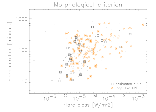
Figure 13: Scatter plot of flare X-ray class versus flare total duration. This plot compares flares associated with XPEs classified according to the morphological criterion. All points are marked with dots. A subset of well-observed (see text) flares are additionally marked with boxes and stars for collimated and loop-like XPEs of high quality (A–B), respectively.

In Fig. 13 we present scatter plot of X-ray class versus total duration for flares associated with morphological subclasses of XPEs, i.e., collimated and loop-like XPEs. All points are marked with dots. Additionally we emphasized well-observed XPEs (quality A or B) and flares that are non-occulted by the solar disk. These flares associated with well-observed collimated and loop-like XPEs are marked with boxes and stars, respectively. Both groups of flares are mixed in the plot, however some shifts toward higher X-ray class and longer duration can be seen for flares associated with loop-like XPEs.

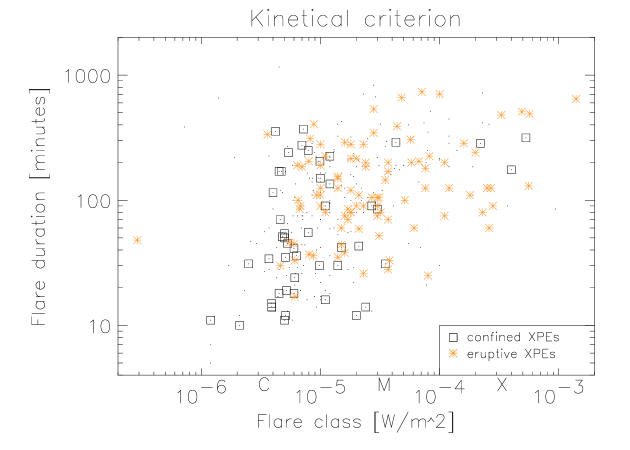
Figure 14: Scatter plot of flare X-ray class versus flare total duration. This plot compares flares associated with XPEs classified according to the kinematical criterion. All points are marked with dots. A subset of well-observed (see text) flares are additionally marked with boxes and stars for confined and eruptive XPEs of high quality (A–B), respectively.

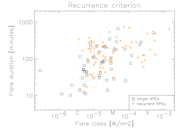
Figure 15: Scatter plot of flare X-ray class versus flare total duration. This plot compares flares associated with XPEs classified according to the recurrence criterion. All points are marked with dots. A subset of well-observed (see text) flares are additionally marked with boxes and stars for single and recurrent XPEs of high quality (A–B), respectively.

Similar scatter plots of X-ray class versus total duration for flares associated with kinematical and recurrence subclasses of XPEs are given in Figs. 14-15. All points are marked with dots. Again, additionally we emphasized well-observed XPEs (quality A or B) and flares that are non-occulted by the solar disk. Moreover, we excluded events for which the assignment of kinematical subclasses for XPEs was uncertain (Fig. 14) and events associated with XPEs that were classified as single in case of partial time-coverage of observations (Fig. 15). In both figures, flares associated with well-observed XPEs classified as subclass 1 (confined and single, respectively) are marked with boxes, whereas flares associated with XPEs classified as subclass 2 (eruptive and recurrent, respectively) are marked with stars. Similarly to Fig. 13, both groups of flares are mixed in the plots and some shifts toward higher X-ray class and longer duration is seen for flares associated with XPEs of subclasses 2.

The shifts seen in Figs. 13-15 are confirmed by medians calculated separately for both groups of flares for each classification criterion. As it is seen in Table 6 (bold-faced columns), medians for flares associated with XPEs of subclass 2 are 1.5–3.8 times and 2.1–2.7 times greater than medians for flares associated with XPEs of subclass 1 for flare X-ray class and flare duration, respectively. Higher X-ray class and longer duration mean a more energetic flare, thus we can conclude that more energetic XPEs are, on average, associated with more energetic flares and less-energetic XPEs rather prefer less-energetic flares.

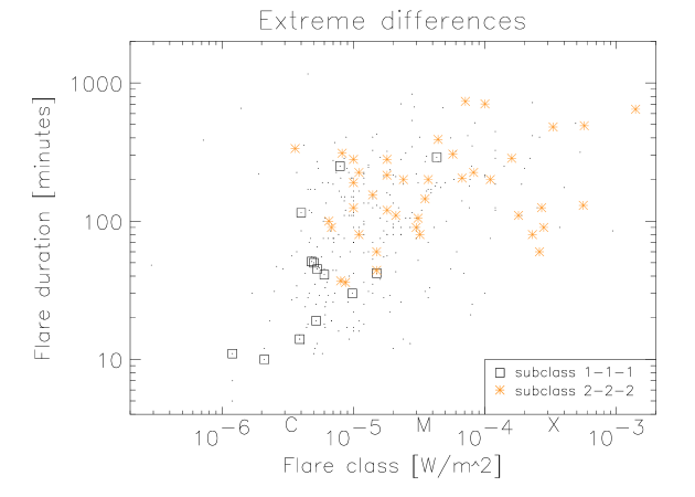
Figure 16: Scatter plot of flare X-ray class versus flare total duration. This plot compares flares associated with XPEs classified according to different criteria that are employed simultaneously. All points are marked with dots. A subset of well-observed (see text) flares are additionally marked with boxes and stars for collimated, confined, single (1,1,1) and loop-like, eruptive, recurrent (2,2,2) XPEs of high quality (A–B), respectively.

One can expect that a difference between characteristics describing associated flares should be even higher for two subclasses of XPEs defined by combining our three criteria simultaneously. Indeed, medians in Table 6 for flares associated with the subclass (1,1,1) – collimated, confined, single XPEs – and the subclass (2,2,2) – loop-like, eruptive, recurrent XPEs – show extreme differences (a factor 6.0 and 3.7 for X-ray class and duration, respectively). As it is seen in Fig. 16, in the diagram X-ray class versus duration, flares associated with the subclasses (1,1,1) and (2,2,2) of well-observed XPEs are almost separated.

In unbold-faced columns in Table 6 we present medians for flares associated with different subclasses of XPEs that were defined less strictly, i.e. by including quality C events and without excluding any doubtful examples. Ratios of medians for subclasses 2 and subclasses 1 that were constituted more liberally are usually lower in comparison with the more strictly defined bold-faced values. It shows how some physical differences can be masked by observational constrains.

3.2 Hard X-rays

We included in the catalogue hard X-ray light curves of associated flares, recorded by Yohkoh HXT, for investigating the relation between XPEs and non-thermal electron signatures. We considered light curves in energy band M1 (23-33 keV) and interpreted a signal above the doubled value of the background as the proof that in a particular flare an acceleration of an appropriate number of non-thermal electrons occurred. For 353 flares which were associated with XPEs we found that 235 events, i.e. 66.6% showed this signature.

In the second and the third columns of Table 6 we present detailed results of this relation for both populations of events and for particular subclasses of XPEs. A percentage of associated flares showing non-thermal electrons depends on how energetic is the subclass, with higher values (75%-82%) for subclasses 2 and lower values (57%-75%) for subclasses 1. The difference is the highest for the kinematical criterion, but for the recurrence criterion percentages for both subclasses are almost the same. After applying all the three criteria we found that the difference between the least energetic subclass (1,1,1) – collimated, confined, single – and the most energetic (2,2,2) – loop-like, eruptive, recurrent – is maximal: 57% and 86% of associated flares indicating non-thermal electrons, respectively.

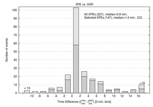
Figure 17: Histogram of time differences between the HXT/M1 light curve maximum and the XPE start. Gray and hatched bins represent the better observed XPEs (quality A-B, so-called selected XPEs) and the rest of XPEs (quality C), respectively. The size of bins is 2 minutes with exception of outermost ones. Numbers of all the considered XPEs and the selected XPEs as well as their medians are given.

We also investigated time coincidence between macroscopic X-ray plasma motions (XPEs) and non-thermal electron signatures (HXRs) in detail. In this aim, we measured time differences between the XPE start and the HXT/M1 flare peak. The results are presented as a histogram in Fig. 17. In 185 from 227 cases (81.5%) XPEs started before the HXR flare peak, in 18.5% of cases the chronology was opposite. However, the most frequent bin: 0–2 minutes in about 45% of cases, suggests that both considered processes, i.e. soft X-ray plasma motion and non-thermal electron acceleration, are strongly coupled.

Similar investigation was performed by Kim et al. (2005a). At first glance our Fig. 17 and their Fig. 5 are different. However, it is needed to know that the values in our histogram have opposite sign and we used the HXR peak time for higher energy band M1, 23-33 keV, than Kim et al. who used energy band L (14-23 keV). In flares with a strong contribution of the non-thermal component, the peak time in those energy bands are close, but in flares with a stronger contribution of the superhot component in L band, the M1 peaks tend to occur earlier than the L peaks. Keeping in mind the above mentioned differences in data organization we can conclude that our results are consistent.

We also prepared variants of Fig. 17 for particular subclasses of XPEs. However, we did not find any evident differences between the considered distributions, namely, each of them shares the common peak bin.

4 XPEs association with Coronal Mass Ejections

In order to associate out XPEs with CMEs, we used the SOHO LASCO CME Catalog (Gopalswamy et al., 2009). Only 275 XPEs occurred when the LASCO coronagraphs were operational. We found that 182 XPEs (66.2%) were associated with CMEs. This is slightly less than 69% (95 from 137 events) obtained by Kim et al. (2005a). For particular subclasses of XPEs the association was between 44% and 88% (see Table 7). According to Yashiro et al. (2008), we consider a XPE-CME pair as physically connected if the XPE occurred within the position angle range defined by the CME angular width increased by 10^∘ from either side. Moreover, the time of the XPE had to fall within 3-hours-interval centered around the extrapolated time of the CME front start at $h=1R_{\sun}$. For the extrapolation we used the time of the first appearance in the LASCO/C2 field of view and the linear velocity taken from the CME catalog.

4.1 Time coincidence

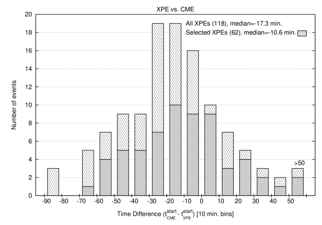
Figure 18: Histogram of time differences between the extrapolated CME front onset and the XPE start. Gray and hatched bins represent the selected subgroup of better observed XPEs (quality A-B, $|\lambda|>60^{\circ}$) and the rest of XPEs, respectively. The size of bins is 10 minutes with exception of outermost right one. Numbers of all the considered XPEs and the selected XPEs as well as their medians are given.

The histogram of the time differences between the extrapolated CME front onset and the XPE start is presented in Fig. 18. As we can see, there are more events with negative values, i.e., those in which the CME starts before the XPE, than those with the opposite chronology. The frequencies are 73.7% (87 from 118) and 26.3% (31 from 118), respectively. The carefully selected subgroup (well-observed XPEs of quality A or B that occurred close to the solar limb, $|\lambda|>60^{\circ}$) shows slightly different proportions: 66,1% (41 from 62) and 33.9% (21 from 62), respectively. Both distributions: all the XPEs and the selected XPEs, are quite gradual with slightly different medians: -17.3 min. and -10.6 min., respectively.

Kim et al. (2005a) performed similar analysis for XPEs from the two-years interval 1999-2001. Their Fig. 6 containing 43 events was made under slightly different assumptions: (1) the CME-front times were extrapolated at individual locations of XPEs in the Yohkoh field of view, (2) the CME speed was determined from the first two observing times and heights. Despite these differences, our histogram looks quite similar to those of Kim et al. Therefore we conclude that, at least in a statistical sense, different ways of extrapolating the CME onset time do not seriously affect the temporal relation between XPEs and CMEs.

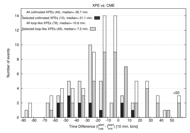
Figure 19: Histogram of time differences between the extrapolated CME front onset and the XPE start made for collimated and loop-like XPEs separately. Black or gray and hatched or white bins represent the selected subgroup of better observed XPEs (quality A-B, $|\lambda|>60^{\circ}$) and the rest of XPEs, respectively. The size of bins is 10 minutes with exception of outermost right one. Numbers of all the considered XPEs and the selected XPEs as well as their medians are given.

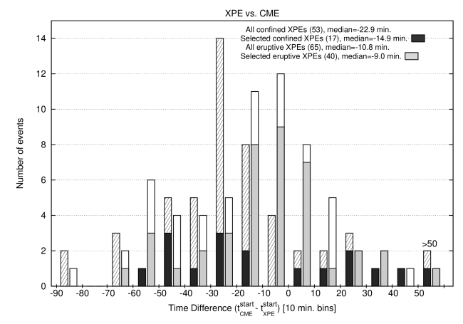
Figure 20: Histogram of time differences between the extrapolated CME front onset and the XPE start made for confined and eruptive XPEs separately. Black or gray and hatched or white bins represent the selected subgroup of better observed XPEs (quality A-B, $|\lambda|>60^{\circ}$) and the rest of XPEs, respectively. The size of bins is 10 minutes with exception of outermost right one. Numbers of all the considered XPEs and the selected XPEs as well as their medians are given.

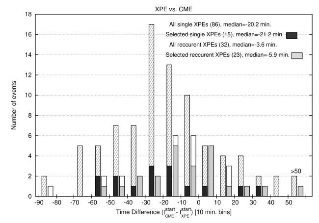
Figure 21: Histogram of time differences between the extrapolated CME front onset and the XPE start made for single and recurrent XPEs separately. Black or gray and hatched or white bins represent the selected subgroup of better observed XPEs (quality A-B, $|\lambda|>60^{\circ}$) and the rest of XPEs, respectively. The size of bins is 10 minutes with exception of outermost right one. Numbers of all the considered XPEs and the selected XPEs as well as their medians are given.

As in the analysis in Section 3.1.1, we give further versions of Fig. 18, in which particular subclasses of XPEs: collimated and loop-like, confined and eruptive, single and recurrent, are separated in Figs. 19, 20, and 21, respectively. In Fig. 19, the histogram for loop-like XPEs shows a relatively narrow maximum located close to the zero point. It means that a large fraction of XPEs ($\sim$50%) starts almost simultaneously with the CME onset. Collimated XPEs are shifted towards negative values in this figure and their maximum is distinctly broader. The histogram made for the selected subgroup of better observed events (gray and black bins in Fig. 19) show a similar trend.

A similar pattern can be seen in Fig. 20. In this Figure the histogram made for eruptive XPEs is narrower and centered closer to the zero point than the histogram made for confined XPEs. The distribution for confined XPEs is much broader, especially in the plot for the selected subgroup of better observed events (black bins), which makes an impression of a random occurrence within almost the whole time window of the CME onset.

In Fig. 21 both histograms made for single and recurrent XPEs show a similar width, but recurrent XPEs tend to start earlier (almost simultaneously with the CME) than single ones. The difference between medians is about 15 minutes for all events as well as for the selected subgroup of better observed events.

4.2 CME angular width and velocity

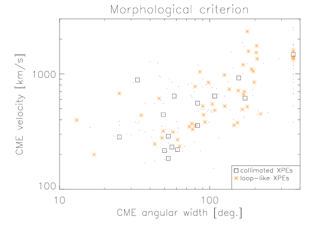
Figure 22: Scatter plot of CME angular width versus CME linear velocity. This plot compares CMEs associated with XPEs classified according to the morphological criterion. All points are marked with dots. A subset of well-observed (see text) CMEs are additionally marked with boxes and stars for collimated and loop-like XPEs of high quality (A–B), respectively. Values are taken from the SOHO LASCO CME catalog (Gopalswamy et al., 2009).

In Fig. 22 we present a scatter plot of an angular width versus a linear velocity for CMEs associated with morphological subclasses of XPEs, i.e., collimated and loop-like XPEs. All points are marked with dots. Additionally we emphasized well-observed XPEs (quality A or B) that occurred close to the solar limb ($|\lambda|>60^{\circ}$). CMEs associated with well-observed collimated and loop-like XPEs are marked with boxes and stars, respectively. Both groups of CMEs are mixed in the plot, however some shifts toward wider and faster events is seen for CMEs associated with loop-like XPEs.

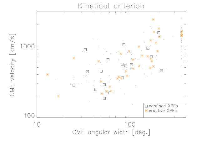
Figure 23: Scatter plot of CME angular width versus CME linear velocity. This plot compares CMEs associated with XPEs classified according to the kinematical criterion. All points are marked with dots. A subset of well-observed (see text) CMEs are additionally marked with boxes and stars for confined and eruptive XPEs of high quality (A–B), respectively. Values are taken from the SOHO LASCO CME catalog (Gopalswamy et al., 2009).

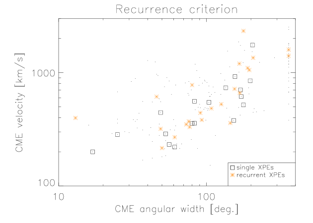
Figure 24: Scatter plot of CME angular width versus CME linear velocity. This plot compares CMEs associated with XPEs classified according to the recurrence criterion. All points are marked with dots. A subset of well-observed (see text) CMEs are additionally marked with boxes and stars for single and recurrent XPEs of high quality (A–B), respectively. Values are taken from the SOHO LASCO CME catalog (Gopalswamy et al., 2009).

Similar scatter plots of an angular width versus a linear velocity for CMEs associated with kinematical and recurrence subclasses of XPEs are given in Figs. 23-24. All points are marked with dots. Again, additionally we emphasized well-observed XPEs (quality A or B) that occurred close to the solar limb ($|\lambda|>60^{\circ}$). Moreover, we excluded events for which the assignment of kinematical subclasses for XPEs was uncertain (Fig. 23) and events associated with XPEs that were classified as single in case of partial time-coverage of observations (Fig. 24). In both figures, CMEs associated with well-observed XPEs classified as the subclass 1 (confined and single, respectively) are marked with boxes, whereas CMEs associated with well-observed XPEs classified as the subclass 2 (eruptive and recurrent, respectively) are marked with stars. Similarly to Fig. 22, both groups of CMEs are mixed in the plots and some shifts toward wider and faster events is seen for CMEs associated with XPEs of the subclasses 2.

The shifts seen in Figs. 22-24 are confirmed by medians calculated separately for both groups of CMEs for each classification criterion. As it is seen in Table 7 (bold-faced columns for well-observed events), the medians for CMEs associated with XPEs of the subclass 2 are 1.2–2.0 times and 1.2–1.4 times greater than those for CMEs associated with XPEs of the subclass 1 for CME angular width and linear velocity, respectively. A higher angular width and velocity mean a more energetic CME, thus we can conclude that more energetic XPEs are, on average, associated with more energetic CMEs and less-energetic XPEs rather prefer less-energetic CMEs.

One can expect that a difference between characteristics describing associated CMEs should be even higher for two subclasses of XPEs that we define by applying our three criteria simultaneously. Indeed, medians in Table 7 for CMEs associated with the subclass (1,1,1) – collimated, confined, single XPEs – and the subclass (2,2,2) – loop-like, eruptive, recurrent XPEs – show extreme differences (factors 2.1 and 1.7 for angular width and linear velocity, respectively). The difference between characteristics describing associated CMEs is also seen in Fig. 25.

In unbold-faced columns in Table 7 we present medians for CMEs associated with different subclasses of XPEs that were defined less strictly, i.e. by including quality C, for $|\lambda|\leq 60^{\circ}$ and without excluding any doubtful examples. Ratios of medians for the subclasses 2 to medians for the subclasses 1 that were constituted more liberally are often comparable to the more strictly defined bold-faced values. It is opposite to flares for which bigger differences between unbold-faced and bold-faced values are evident (see Table 6). We suggest that the main reason for this is the condition $|\lambda|>60^{\circ}$, that we constituted for specially selected (bold-faced) events. It excludes the majority of halo CMEs being systematically wider and faster than ordinary CMEs (Michałek et al., 2003). In other words, more strict selection criteria undoubtedly limit a scatter of values in two physically different groups, however it is compensated with the bias introduced by halo CMEs.

5 Discussion

The XPEs collected in the catalogue confirm the strong association with flares. Starts of XPEs observed since their very beginning fall usually within the rising phase of associated flares (Figs. 3 and 5) and well coincide with the HXR peaks (Fig. 17). It means that symptoms of SXR plasma motions occur when magnetic energy conversion in flares – via reconnection – is most vigorous (Benz, 2008). A small number of exceptions is connected mainly with complex events in which X-ray enhancements, recorded by GOES and Yohkoh/HXT, are accumulated from at least two different positions on the Sun.

We would like to stress a lower correlation between XPEs and HXR flares than between XPEs and SXR ones. As approximately one third of flares associated with XPEs did not show any clear signatures of non-thermal electrons, we can conclude that some macroscopic motion of SXR plasma is more obvious characteristics of reconnection than acceleration of non-thermal electrons. It can be caused by the the limited sensitivity of the HXT. As we can see in Table 6, the more energetic subclasses 2 in our classification scheme of XPEs show a stronger correlation with HXR flares. Thus, under the assumption that the more energetic XPEs are associated with more energetic flares, we can expect a larger fraction of them to be able to produce the HXR emission above the threshold of the HXT.

Another proof of close association between processes responsible for XPEs and flares is similarity between their durations. A comparison between the medians in Figs. 5 and 9 shows that an XPE lasts, on average, as long as the rising phase of an associated flare. Histograms presented for particular subclasses of XPEs (Figs. 6-8 and 10-12) show that the more energetic subclasses 2 occur earlier and last shorter than the less energetic subclasses 1. This difference probably reflects some differences in reconnection processes occurring in both subclasses. At first sight, this result is in contradiction with Figs. 13-15, in which XPEs from subclasses 2 seem to prefer flares of longer duration, however we should remember that in Figs. 6-8 and 10-12 the time is normalized with the flare rising-phase duration.

Some interesting hints concerning hierarchy and chronology of processes occurring in restructuring active regions can be found in histograms of time differences between the XPE start and the extrapolated CME onset for particular subclasses of XPEs (Figs. 19-21). The more energetic subclasses 2 of XPEs show close relationship with their associated CMEs. They seem to start almost simultaneously, and small deviations from the zero value are probably caused by unrealistic extrapolation of the CME onsets. The start of XPEs of the less energetic subclasses 1 shows a much looser connection with the CME start. Very often the CME seems to occur first. Keeping in mind that XPEs are usually caused by magnetic reconnection, we suggest that in the case of the subclasses 2, the reconnection and loss-of-equilibrium of magnetic structure, thus a CME development, occur almost simultaneously. On the other hand, in the case of the subclasses 1, the reconnection is usually a consequence of destabilization of magnetic structure, which may occur earlier.

The results summarized in Tables 6 and 7 strongly suggest that total amount of energy, converted from the magnetic field in an active region during its magnetic reconfiguration, determines characteristics of events including flares, CMEs, and XPEs, which are thought to be consequences of this common reconfiguration. Thus, more energetic XPEs are associated with more energetic flares and CMEs, while less energetic ones – seem to occur commonly. This statistically averaged picture does not exclude, for sure, exceptions in partitioning of magnetic energy. For example, there are X-class confined flares completely devoid of any CME (Wang & Zhang, 2007; Cheng et al., 2011). These flares are probably also devoid of XPEs but this research is beyond the scope of this work.

Our investigation shows that characteristics of flares and CMEs associated with particular subclasses of XPEs are different. We found that a scale of differences is higher for flares than for CMEs. We also found that the recurrence criterion proposed in our XPE classification scheme does not separate the associated events as strongly as the morphological and kinematical criteria.

6 Conclusions

In our catalogue we have collected the most extensive database of XPEs so far. Images from the SXT onboard Yohkoh have been organized into movies in the MPEG format. The events have been classified on the basis of elementary and uniform criteria. The catalogue also gives a piece of information concerning the associated flares and CMEs by using entries to the Yohkoh Flare Catalogue (HXT/SXT/SXS/HXS) and the SOHO LASCO CME Catalog, respectively. The collected data allow us to study XPEs more comprehensively as a separate solar activity phenomena and also as elements of more complex processes occurring in the solar corona.

XPEs constitute a strongly inhomogeneous group of events. Their appearances include expanding loop structures, moving blobs, rising columns, and so on. Their strong inhomogeneity is responded by wide range of values of basic parameters: altitude ($10^{8}-10^{10}$ cm), volume ($10^{26}-10^{30}$ cm^-3), duration ($10^{1}-10^{3}$ s), velocity ($10^{0}-10^{3}$ km s^-1), acceleration ($-10^{3}-10^{4}$ m s^-2), mass ($10^{12}-10^{15}$ g), energy ($10^{25}-10^{31}$ ergs).

It is difficult to point out a universal mechanism responsible for all the events presented in the catalogue. There is no doubt that the majority of XPEs is connected somehow with magnetic reconnection. However, in many events, the evolution is far from what may be expected from the canonical CSHKP model, suggesting the existence of more complex 3D quadrupolar reconnection (Nitta, Freeland & Liu, 2010). We often observe an XPE as a result of magnetic reconnection that leads to chromospheric evaporation as a hydrodynamic response of intensified plasma heating or non-thermal electron beams in a flare magnetic structure.

On the other hand, the close morphological and kinematical connection of some XPEs with CMEs, together with the similar start time, suggests a mechanism of loss-of-equilibrium type common for CMEs. [Indeed, movies illustrating evolution of some XPEs resemble cartoons presenting the tether release model or the tether straining model leading to the magnetic breakout model.] Finally, some movies in the catalogue give an impression that SXR plasma leaks out from the magnetic structure probably under low-$\beta$-plasma conditions.

For proper interpretation of the data, we need to identify the mechanism responsible for the observed XPE. An inappropriate choice of the mechanism can lead to meaningless and erroneous conclusions regarding processes occurring in the solar corona. In the context of strong inhomogeneity of XPEs and several possible mechanisms of their origin, it is not advised to routinely interpret all XPEs in terms of a single and same mechanism. The similar conclusion were given by Nitta, Freeland & Liu (2010) who criticized the tendency to employ the CSHKP model for description all “Masuda-type” flares (Masuda et al., 1994).

If we consider a one particular XPE, it is basically difficult to decide which mechanism is responsible for its occurrence without the complete quantitative analysis including plasma diagnostics and a modeling of magnetic field structure. These conditions were unreachable in practice for the majority of events in the catalogue. Therefore, in advent of new observations of XPEs derived by modern instruments onboard Hinode, Solar-Terrestrial Relations Observatory (STEREO), and the Solar Dynamics Observatory (SDO), we have been trying to give some solutions that would be correct at least in statistical sense.

We have shown that the subclasses of XPEs separated on the basis of our simple observational criteria have different levels of correlation with other solar-activity phenomena. The difference is also seen if we consider basic parameters describing these flares and CMEs. However, the association of XPEs with different flares or CMEs does not mean a specific physical mechanism as far as these flares or CMEs represent physically different groups. In the meantime, discussions concerning a difference in observational characteristics to justify separate physical mechanisms responsible for flares or CMEs are still open. Are there two different classes of flares (Pallavicini, Serio & Vaiana, 1977) or all flares can be explained by only one mechanism (Shibata et al., 1995)? Are there two kinematically different classes of CMEs (Sheeley et al., 1999) or the division is artificial (Vr$\check{\rm{s}}$nak, Sudar & Ru$\check{\rm{z}}$djak, 2005)?

We have found that more energetic XPEs are better correlated with flares and CMEs and that more energetic XPEs correlate with more energetic flares and CMEs. Virtually the effect of observational conditions works in the same way and we cannot resolve correctly the influence of the effect on our conclusion.

The most promising way in the investigation of XPEs is to deal them as an element of a larger ensemble. The usage of observations made in temporal, spatial, and spectral ranges broader than those needed for direct monitoring of XPEs allows the better understanding of processes in which XPEs participate. Recently, a similar picture of flares as global events was presented by Hudson (2011). Our experience is that XPEs are strongly coupled with flare HXR quasi-periodic oscillations (Nakariakov & Melnikov, 2009), probably because the reconnection rate is controlled by plasmoid generation (Nishida et al., 2009). We also found that XPEs are somehow associated with progressive spectral hardening in HXRs (Tomczak, 2008), thus with Solar Energetic Particles (Kiplinger, 1995; Grayson, Krucker & Lin, 2009).

In the future we are going to upgrade the XPEs catalogue by adding entries devoted to associated prominences and radio bursts. Moreover, the TRACE movies will be added, if available. We also are going to perform the comprehensive analysis of several, very interesting events from the catalogue that have been omitted by other Yohkoh researchers.

Figure 25: Scatter plot of CME angular width versus CME linear velocity. This plot compares CMEs associated with XPEs classified according to different criteria that are employed simultaneously. All points are marked with dots. A subset of well-observed (see text) CMEs are additionally marked with boxes and stars for collimated, confined, single (1,1,1) and loop-like, eruptive, recurrent (2,2,2) XPEs of high quality (A–B), respectively. Values are taken from the SOHO LASCO CME catalog (Gopalswamy et al., 2009).

Table 1: XPEs presented in the catalogue

No.	Date	Time	Class.	Q.	AR	GOES	Coordinates	CME	References
001	91/10/22	06:42.2-07:28.8	2,1,2	B	6891	M1.2	S11 E85	$\cdots$	19
002	91/11/02	16:31.2-16:57.3	2,2,1	B	6891	M4.8	S10 W84	$\cdots$	19
003	91/11/17	18:32.9-18:41.8	1,1,2	C	6929	M1.9	S12 E78	$\cdots$	19
004	91/12/02	04:50.6-05:21.0	2,2,1	A	6952	M3.6	N18 E92	$\cdots$	18,19,27,28,54
005	91/12/03	16:35.0-17:04.5	2,1,1	B	6952	X2.2	N17 E72	$\cdots$	19
006	91/12/09	02:02.7-02:06.5	2,1,1	C	6966	M1.4	S06 E91	$\cdots$	19
007	91/12/10	04:03.0-04:10.1	1,1,1	B	6968	C9.3	S14 E93	$\cdots$	19
008	92/01/13	17:27.9-17:35.2	2,2,2	C	6994	M2.0	(S15 W89)	$\cdots$	18,19,27,28
009	92/01/13	19:04.1-19:13.8	1,2,1	C	7012	M1.3	S10 E95	$\cdots$	19
010	92/01/14	19:29.0-19:32.6	2,2,1	B	7012	M1.7	S11 E89	$\cdots$	19
011	92/01/15	18:56.1-19:04.5	2,2,1	B	7012	M2.0	(S09 E72)	$\cdots$	19
012	92/01/30	17:07.6-17:17.6	2,1,1	C	7042	M1.6	S13 E84	$\cdots$	19
013	92/02/06	03:17.4-03:36.6	2,2,1	B	7030	M7.6	N05 W82	$\cdots$	18,19,27,28
014	92/02/06	20:52.7-21:24.8	2,2,1	B	7030	M4.1	N05 W94	$\cdots$	19
015	92/02/09	03:01.0-03:10.7	2,1,1	C	7035	M1.2	S17 W74	$\cdots$	19
016	92/02/17	15:41.8-16:25.0	1,2,2	C	7050	M1.9	N16 W81	$\cdots$	18,19,27,28
017	92/02/18	18:00.1-18:29.9	2,1,1	C	7067	+	(N05 E89)	$\cdots$	13
018	92/02/19	14:45.4-15:39.1	2,2,1	B	7067	M1.2	N06 E94	$\cdots$	19
019	92/02/21	03:11.9-03:19.2	2,1,1	C	7070	M3.2	(N09 E80)	$\cdots$	19
020	92/02/21	22:04.6-22:08.0	2,1?,1	C	7070	M2.2	N05 E65	$\cdots$	19
021	92/04/01	10:12.8-10:22.5	2,2,1	B	7123	M2.3	(S03 E89)	$\cdots$	18,27,28
022	92/06/05	18:08.7-19:08.9	2,1,1,	C	7186	C2.6	N07 E28	$\cdots$	13
023	92/06/07	01:41.0-01:50.0	2,2,1	B	7186	M2.7	N09 E10	$\cdots$	4
024	92/07/20	17:18.1-17:49.6	1,1,1	C	7222	–	(S06 W88)	$\cdots$	13
025	92/07/29	20:19.7-21:09.8	2,2,2	B	7236	–	(N19 W88)	$\cdots$	13
026	92/08/25	19:02.6-19:36.4	1,1,1	B	7260	C8.7	N13 W98	$\cdots$	19
027	92/09/09	02:06.2-02:18.6	1,1,1	C	7270	M3.1	S10 W72	$\cdots$	19
028	92/09/09	17:57.9-18:07.2	1,2?,1	C	7270	M1.9	S11 W78	$\cdots$	19
029	92/10/04	22:14.0-22:32.4	2,2,2	B	7293	M2.4	S05 W90	$\cdots$	18,19,24,27,28,53
030	92/10/05	09:24.3-09:52.0	1,2,1	B	7293	M2.0	S08 W90	$\cdots$	10,12,18,19,21,24,53
031	92/11/05	06:19.0-06:40.7	$\cdots$	D	7323	M2.0	S16 W90	$\cdots$	18,19,27,28
032	92/11/05	20:30.1-21:08.6	$\cdots$	D	7323	C8.7	S17 W92	$\cdots$	19
033	93/02/14	12:51.9-12:59.4	2,2,1	B	7427	M2.0	S22 E78	$\cdots$	19
034	93/02/17	10:35.4-10:53.5	1,2,1	B	7420	M5.8	S07 W87	$\cdots$	14,18,19,24,27,28,53
035	93/02/21	00:31.2-00:45.2	2,2,1	B	7433	M1.4	N13 E75	$\cdots$	19
036	93/03/15	20:31.9-21:15.2	2,2,1	B	7440	M2.9	S03 W93	$\cdots$	4
037	93/03/23	01:21.0-01:29.5	2,2,1	B	7448	M2.3	N18 W78	$\cdots$	4
038	93/05/07	20:56.6-21:30.6	2,2,1	B	7500	M1.6	N14 E41	$\cdots$	4
039	93/05/14	22:00.1-22:10.3	2,2,1	A	7500	M4.4	N19 W48	$\cdots$	23
040	93/06/25	03:13.8-03:40.3	2,2,1	B	7530	M5.1	S09 E88	$\cdots$	19
041	93/06/28	01:06.7-01:23.0	2,2,2	B	7535	C6.5	N03 E69	$\cdots$	6
042	93/09/26	17:26.2-17:28.3	2,1,1	B	7590	C3.4	N14 E94	$\cdots$	19
043	93/09/27	12:07.5-12:17.8	2,2,1	B	7590	M1.8	N08 E90	$\cdots$	18,19
044	93/10/01	23:51.3-00:01.3	2,1,1	C	7592	C8.5	S14 E69	$\cdots$	19
045	93/11/11	11:15.4-11:31.8	1,2,1	B	7618	C9.7	N10 E95	$\cdots$	10,14,20
046	93/11/13	06:38.6-06:48.9	1,2?,1	B	7618	M2.1	N08 E73	$\cdots$	19
047	94/01/05	06:49.4-06:59.6	2,2?,1	B	7647	M1.0	S13 W23	$\cdots$	4
048	94/01/16	23:09.6-23:22.9	2,2,1	B	7654	M6.1	N05 E71	$\cdots$	19
049	94/01/27	03:47.8-03:59.0	1,1,1	B	7654	C4.6	N08 W68	$\cdots$	4
050	94/01/28	16:53.2-17:26.5	2,2,2	B	7654	M1.8	N08 W85	$\cdots$	19
051	94/02/27	09:02.7-09:18.9	2,2,1	B	7671	M2.8	N08 W98	$\cdots$	4
052	94/08/30	08:20.5-08:41.4	1,1,1	B	7773	M1.1	S06 E82	$\cdots$	19
053	96/04/20	06:51.7-07:04.4	1,2,1	A	7956	B2.9	N04 W68	$\cdots$	24,36,53
054	96/08/22	07:42.5-07:52.1	2,2,1	B	7986	C4.5	S14 E107	+	3,50,52
055	97/02/23	01:30.2-02:15.2	2,2?,1	B	8019	B7.2	(N31 E90+)	–	2
056	97/02/23	02:58.2-03:31.0	2,1,1	C	8019	B7.2	(N33 E81)	+	4
057	97/05/16	11:44.0-12:10.7	1,2,1	C	8038	–	(N20 W73)	+	4
058	97/08/09	16:32.9-16:35.3	1,2?,1	C	8069	C8.5	N19 W85	+	16,19
059	97/09/17	11:38.4-11:49.2	1,2,1	B	8084	M1.7	N21 W82	+	16,19
060	97/09/17	17:48.4-18:24.6	2,2,2	B	8084	M1.0	N21 W84	+	19
061	97/11/06	11:50.8-12:06.3	2,2,1	C	8100	X9.4	S18 W63	+	17,48
062	97/11/14	09:11.0-09:20.8	2,1,1	B	8108	C2.5	N21 E70	+	24,48,53
063	97/11/27	13:10.4-13:25.2	2,2,2	A	8113	X2.6	N17 E63	+	29,48
064	98/03/23	02:45.9-03:12.1	2,2,2	B	8179	M2.3	S22 W99	+	16,19,50
065	98/03/25	13:04.1-13:17.1	2,2,1	C	8180	C5.3	(S37 W90+)	+	2
066	98/04/20	09:43.8-10:12.5	2,2?,2	C	8194	M1.4	S30 W90	+	17
067	98/04/23	05:29.4-05:46.8	2,2,2	A	8210	X1.2	S18 E104	+	1,10,16,18,19,24,26,
									50,51,52,53
068	98/04/24	08:47.6-08:55.2	2,1,1	C	8210	C8.9	S20 E91	+	19
069	98/04/25	14:21.9-14:49.2	2,2,2	B	8210	C3.6	S19 E73	+	2
070	98/04/27	08:50.0-08:55.3	2,2?,1	B	8210	X1.0	S16 E50	+	34
071	98/05/03	21:17.4-21:25.5	2,2,2	A	8210	M1.4	S13 W34	+	30
072	98/05/06	07:54.3-08:11.0	2,2,2	A	8210	X2.7	S11 W65	+	17,24,35,48,53
073	98/05/08	01:50.4-02:20.1	2,2,2	A	8210	M3.1	(S16 W90+)	+	16,18,19
074	98/05/08	14:21.2-14:49.4	2,2,2	B	8210	M1.8	S17 W95	+	19
075	98/05/09	02:04.7-02:20.1	1,2,1	C	8210	C7.0	(S15 W90+)	–	16
076	98/05/09	03:17.7-03:37.3	2,2,2	A	8210	M7.7	S17 W102	+	16,18,19,50
077	98/05/10	13:25.4-13:33.2	2,2?,1	B	8220	M3.9	S27 E89	–	19
078	98/05/28	06:22.5-06:28.2	1,1,1	B	8226	C1.2	N20 W78	–	19
079	98/05/28	19:02.4-19:17.6	2,2,2	B	8226	C8.7	(N16 W87)	+	16,19
080	98/05/29	01:02.8-01:12.0	1,2,1	C	8226	M6.7	(N15 W89)	+	19
081	98/06/11	10:00.8-10:18.3	2,2,2	C	8243	M1.4	(N21 E89)	+	16,50
082	98/06/15	07:26.8-07:34.3	2,2,1	C	8232	C1.4	(S16 W87)	+	2
083	98/07/03	01:06.5-01:12.7	2,2?,1	C	8256	M1.2	S26 W14	$\cdots$	4
084	98/08/14	08:25.5-08:31.7	2,2,1	B	8293	M3.1	S23 W74	$\cdots$	19
085	98/08/18	08:17.5-08:26.5	2,2,2	B	8307	X2.8	N33 E68	$\cdots$	18,19,48
086	98/08/18	22:15.1-22:20.7	2,2,1	B	8307	X4.9	N33 E87	$\cdots$	18,19,31,48
087	98/09/06	02:12.3-02:18.5	1,1?,1	B	8323	C2.3	S22 W35	$\cdots$	4
088	98/09/20	02:38.5-03:19.1	2,2,2	B	8340	M1.8	N22 E62	$\cdots$	4
089	98/09/23	00:30.2-00:47.6	2,2,1	B	8344	C9.3	S20 E22	$\cdots$	4
090	98/09/23	06:45.3-07:05.2	2,2,2	B	8340	M7.1	N18 E09	$\cdots$	40
091	98/09/28	16:07.9-16:11.7	2,2,1	C	8339	C6.8	(S15 W87)	$\cdots$	4
092	98/09/30	13:16.4-13:40.5	1,2,2	B	8340	M2.8	N23 W81	$\cdots$	4
093	98/10/07	17:08.6-17:44.8	2,2,1	A	8355	M2.3	S23 E68	$\cdots$	32
094	98/10/20	20:34.5-21:16.1	2,2,2	C	8360	C7.4	(S21 W86)	$\cdots$	4
095	98/11/03	19:14.3-19:36.3	2,1?,2	B	8375	M1.0	N21 E02	+	4
096	98/11/05	01:03.4-01:12.2	2,1,2	C	8375	C7.1	(N20 W14)	+	33
097	98/11/06	02:42.1-02:51.8	1,1,1	C	8375	C4.4	N19 W24	–	4
098	98/11/06	09:09.9-09:16.6	1,1?,1	C	8375	C4.2	N19 W27	+	4
099	98/11/07	17:52.1-18:01.1	1,2?,1	B	8375	C5.3	N19 W48	–	4
100	98/11/16	23:11.4-23:18.7	2,2,2	B	8385	C6.8	(N24 W83)	$\cdots$	4
101	98/11/22	06:39.6-06:47.2	2,2,2	C	8384	X3.7	S27 W82	$\cdots$	28,34
102	98/11/22	16:21.5-16:31.1	1,2,2	B	8384	X2.5	S30 W89	$\cdots$	28,34
103	98/11/24	02:19.6-02:28.3	2,2,1	C	8384	X1.0	S30 W103	+	4
104	98/11/25	14:00.8-14:07.5	2,2,1	C	8395	C6.4	N18 E68	+	4
105	98/11/28	05:29.5-05:49.6	2,2,2	B	8395	X3.3	N17 E32	+	34,48
106	98/12/18	17:17.5-17:27.9	2,2,1	C	8414	M8.0	(N34 E40)	+	4
107	98/12/23	05:53.5-06:02.9	2,1,1	C	8414	M2.3	(N28 E70)	$\cdots$	4
108	98/12/24	01:22.2-01:29.1	2,1,1	C	8421	C6.2	N29 E85	$\cdots$	4
109	98/12/25	06:18.4-06:35.0	2,1?,2	B	8421	M1.2	N30 E66	$\cdots$	4
110	98/12/28	05:16.2-05:31.9	2,1,2	B	8416	M1.4	N28 E26	$\cdots$	4
111	99/01/03	08:15.4-09:03.8	2,2,2	A	8420	C8.2	N16 W70	$\cdots$	4
112	99/01/06	23:59.7-00:05.4	1,2,1	B	8422	C8.0	(S23 W90)	$\cdots$	4
113	99/01/14	10:06.9-10:17.0	2,2,1	B	8439	M3.0	N18 E64	$\cdots$	4
114	99/02/10	23:09.1-23:25.3	2,2?,1	C	8457	C3.7	(N18 E57)	+	4
115	99/02/12	15:23.7-15:32.1	2,2?,1	B	8456	C5.7	N12 E27	–	4
116	99/02/16	21:19.7-21:27.8	2,2,2	C	8462	C5.3	N19 W12	$\cdots$	4
117	99/02/21	13:16.0-13:41.5	1,1?,2	B	8462	M1.3	N24 W81	–	4
118	99/03/07	04:05.5-04:11.9	2,2,1	C	8477	C2.9	N24 W03	+	4
119	99/04/03	23:02.0-23:10.5	1,1,1	B	8508	M4.3	N29 E81	+	9
120	99/05/07	04:31.5-04:45.0	2,2,2	A	8535	M3.2	N20 E87	+	9,10
121	99/05/08	14:33.0-14:52.1	1,1,1	C	8526	M4.6	N23 W75	+	9
122	99/05/09	12:34.7-13:05.5	2,1?,2	C	8526	M1.0	(N22 W84)	+	9
123	99/05/09	18:04.2-18:17.3	1,2,1	B	8526	M7.6	(N22 W86)	+	8,9
124	99/05/11	21:46.9-22:02.7	2,1,1	C	8542	C4.7	S19 E79	+	9
125	99/05/16	17:26.2-17:32.9	1,1,1	B	8534	M1.1	S17 W76	–	9
126	99/05/17	03:43.2-03:51.6	1,1,2	B	8534	C3.9	(S16 W82)	–	8,9,24,37,53
127	99/05/17	04:57.5-05:01.0	1,1,1	C	8534	M2.3	(S15 W82)	–	9
128	99/05/29	03:08.1-03:14.2	2,2,1	B	8557	M1.6	(S21 E65)	+	9
129	99/06/11	11:25.4-11:38.4	2,2,1	B	8585	C8.8	(N46 E90)	+	9
130	99/06/19	22:31.8-22:42.8	2,1,1	C	8592	C4.0	(N25 E86)	+	9
131	99/06/23	00:41.2-00:51.0	2,1,1	B	8583	C7.9	S12 W78	+	9
132	99/06/30	03:11.0-03:18.3	1,1,1	C	8613	C4.5	(N19 E90)	+	9
133	99/06/30	04:36.2-05:00.8	2,2,2	B	8611	M2.1	S26 E28	+	4
134	99/07/07	06:20.7-06:30.3	1,2?,1	C	8611	C1.2	S26 W76	+	9
135	99/07/07	09:19.1-09:24.4	1,1,1	C	8611	C1.2	(S26 W76)	+	9
136	99/07/09	22:38.5-22:48.2	1,1,1	C	8629	C6.9	N22 W69	–	9
137	99/07/12	23:31.9-23:38.0	1,1,1	B	8626	C2.1	(S19 W76)	–	9
138	99/07/16	15:50.8-15:55.3	1,1,1	C	8635	M3.1	N43 W71	+	9
139	99/07/23	04:45.9-05:03.8	2,1,1	B	8645	C9.3	S23 E97	–	9
140	99/07/23	15:56.1-16:26.3	1,1,1	C	8645	M1.0	S26 W92	–	9
141	99/07/23	22:58.1-23:10.9	2,1,1	C	8644	M1.2	S26 E87	–	9
142	99/07/24	03:31.7-04:06.6	2,1,1	C	8636	M1.7	S29 E87	–	9
143	99/07/24	08:00.4-08:16.7	2,1?,1	B	8636	M3.3	S28 E78	+	9
144	99/07/25	13:08.8-13:14.7	2,2,1	B	8639	M2.4	N38 W81	+	8,9,10,24,38,53
145	99/08/04	05:58.5-06:11.5	2,1,1	C	8647	M6.0	S16 W64	+	9
146	99/08/04	21:54.2-22:03.2	1,1,1	C	8647	C3.3	(S18 W80)	–	9
147	99/08/06	10:05.3-10:18.0	2,1,1	C	8647	C7.1	S28 W81	+	9
148	99/08/07	20:52.0-21:10.9	2,2,2	B	8645	M1.7	S29 W104	+	9
149	99/08/10	06:02.4-06:13.2	1,1,1	C	8656	C4.8	N15 W74	–	9
150	99/08/13	15:07.9-15:16.2	1,1,1	B	8668	C5.3	(N17 E90)	–	9
151	99/08/14	12:06.0-12:16.9	1,1,1	C	8668	C7.2	N23 E72	–	9
152	99/08/20	12:40.4-13:36.6	2,2?,2	C	8674	M1.8	S28 E76	+	9
153	99/08/28	17:54.1-18:04.6	2,2,2	B	8674	X1.1	S26 W14	+	48
154	99/09/08	12:13.6-12:14.5	2,2?,1	C	8690	M1.4	N12 E53	+	25
155	99/09/21	10:16.0-10:34.6	2,2,1	B	8692	C6.4	(S25 W84)	+	9
156	99/10/25	19:37.8-19:44.1	2,2,1	C	8737	C4.8	S19 W69	+	9
157	99/10/26	21:12.0-21:27.6	2,2,2	B	8737	M3.7	(S16 W86)	+	9,10,11,18,28,39
158	99/10/27	09:11.2-09:13.9	2,2,1	B	8737	M1.0	S12 W88	–	9
159	99/10/27	13:35.2-14:04.9	2,2,1	B	8737	M1.8	S15 W90	+	9
160	99/10/27	15:21.1-15:43.6	2,1,1	B	8737	M1.4	S14 W92	+	9
161	99/11/05	18:22.5-18:48.6	2,2?,1	B	8759	M3.0	N12 E96	+	9,10
162	99/11/06	06:32.5-06:35.1	1,1,1	C	8759	C4.6	(N12 E86)	–	8,9
163	99/11/06	17:04.4-17:14.4	1,1,1	B	8759	C5.0	(N12 E86)	+	9
164	99/11/08	06:06.0-06:16.0	$\cdots$	D	8749	C5.9	S18 W82	+	9
165	99/11/13	02:22.7-03:09.4	2,2?,1	C	8763	M1.3	S15 E44	+	9
166	99/11/27	12:12.1-12:23.3	1,1,1	C	8771	X1.4	S15 W68	+	9,48,49
167	99/12/18	01:26.8-01:39.1	2,2,1	C	8806	C9.4	N19 E82	–	9
168	00/01/12	20:50.0-20:56.9	2,2,2	B	8829	M1.1	N13 E67	+	9
169	00/01/18	09:36.0-09:58.8	1,2,1	A	8827	M1.2	S15 W106	+	9,10,24,53
170	00/01/18	17:12.1-17:18.1	2,2?,1	C	8831	M3.9	S19 E11	+	4
171	00/01/22	17:58.9-18:08.8	2,1,2	C	8831	M1.0	S23 W50	+	4
172	00/02/04	09:14.6-09:57.4	2,1,1	C	8858	M3.0	N25 E71	–	28
173	00/02/04	19:28.3-19:43.5	1,2,2	B	8858	C7.0	N25 E71	+	9
174	00/02/05	19:33.9-19:43.9	2,1?,2	B	8858	X1.2	N26 E52	+	48
175	00/02/22	20:26.2-21:24.0	2,1,1	C	8882	C9.2	(S18 E90+)	+	9
176	00/02/26	23:38.5-23:43.8	2,2,2	B	8889	M1.0	N29 E50	–	4
177	00/03/02	08:23.7-08:28.7	2,2,1	B	8882	X1.1	(S18 W55)	+	48,49
178	00/03/02	13:12.5-13:20.5	1,2,1	C	8882	C5.5	S19 W60	+	4
179	00/03/03	02:11.6-02:14.6	2,2,1	B	8882	M3.8	S15 W60	+	4
180	00/03/06	10:47.9-10:50.0	1,1,1	B	8889	C4.5	(N20 W75)	–	9
181	00/03/06	16:20.0-16:28.4	2,1,1	B	8889	C3.9	N20 W78	–	9
182	00/03/18	20:50.7-20:57.3	2,2,1	B	8906	M2.1	(S15 W68)	+	4
183	00/03/18	21:53.5-21:59.0	1,1,1	B	8906	C4.2	S19 W67	+	4
184	00/03/18	23:16.9-23:27.4	2,1,1	B	8902	+	(S18 E90+)	+	9
185	00/03/27	13:59.1-14:25.5	$\cdots$	D	8926	C8.4	S09 W69	–	9
186	00/03/27	15:32.8-15:41.9	2,1,1	C	8926	C8.9	S10 W69	–	24
187	00/03/31	06:27.8-06:50.8	2,2?,1	B	8936	M1.2	S15 E55	+	9
188	00/04/06	02:22.4-02:31.9	2,2,1	B	8948	M1.8	S15 E53	+	4
189	00/04/08	02:37.5-02:47.5	2,2,1	C	8948	M2.0	S15 E26	+	4
190	00/05/02	14:53.2-15:03.0	1,1,2	C	8971	M2.8	N22 W68	+	9
191	00/05/05	15:18.3-15:47.5	2,2,2	B	8977	M1.5	S18 W110	+	9
192	00/05/12	08:40.9-08:50.7	$\cdots$	D	8998	C8.1	S14 E90	–	9,41
193	00/05/12	21:32.8-21:39.8	$\cdots$	D	8998	C9.8	S15 E81	–	9
194	00/05/13	01:46.6-02:10.1	2,2,1	C	9002	M1.1	N22 E109	–	9
195	00/05/13	23:12.4-23:21.8	2,1,1	C	9002	C7.4	N22 E96	+	9
196	00/05/15	08:26.8-08:53.1	2,2,1	C	9002	M4.4	(N23 E87)	+	9
197	00/05/18	15:55.6-16:05.0	2,2?,1	C	9002	M2.7	N23 E30	+	4
198	00/05/23	17:50.1-18:00.1	1,1,1	C	8996	C4.3	S22 W80	+	9
199	00/05/24	00:09.2-00:19.1	1,1,1	C	9017	C6.8	(S12 E90+)	–	9
200	00/05/24	03:14.3-04:02.8	1,1,1	C	9017	C7.0	S12 E93	–	9
201	00/05/24	11:43.3-12:13.0	1,1,1	C	9017	M1.1	(S12 E90)	–	9
202	00/05/24	21:05.6-21:51.1	1,1,1	C	9017	C9.7	(S12 E90)	–	9
203	00/05/26	11:33.1-11.37.6	2,2?,1	B	8998	C6.1	S13 W90	+	9
204	00/05/28	10:23.6-10:34.6	1,1,1	C	9002	C8.6	(N21 W88)	+	9
205	00/06/02	03:44.6-03:50.8	2,1,1	B	9026	M1.2	(N22 E77)	+	9
206	00/06/02	20:32.7-21:10.3	2,1,1	B	9026	M3.1	(N21 E67)	+	9
207	00/06/06	15:35.6-15:45.6	1,1,1	C	9026	X2.3	(N20 E18)	+	4
208	00/06/07	15:42.9-15:52.9	2,2?,1	B	9026	X1.2	N23 E03	+	4
209	00/06/12	12:24.4-12:57.5	2,1,1	C	9042	C6.4	N16 E87	–	9
210	00/06/17	02:29.6-02:45.3	1,1,2	C	9033	M3.5	N22 W72	+	9
211	00/06/18	02:04.4-02:14.4	1,2,1	C	9033	X1.0	N23 W85	+	9
212	00/06/19	04:18.1-04:23.0	1,1,1	C	9033	C1.7	(N21 W89)	+	9
213	00/06/21	09:24.5-09:34.1	1,1,1	C	9042	M1.3	N24 W42	+	4
214	00/06/23	14:22.7-14:37.9	2,2,1	B	9042	M3.0	N26 W72	+	9
215	00/06/23	22:14.9-22:24.8	1,1?,2	C	9042	C7.7	N22 W74	+	9
216	00/06/28	12:17.4-12:19.5	2,1?,1	B	9064	C6.1	(S22 W73)	–	9
217	00/06/29	10:28.6-10:38.7	1,1,1	B	9064	C4.8	(S17 W82)	–	9
218	00/07/01	12:37.6-12:43.1	1,1,1	B	9054	C6.0	(N15 W75)	–	9
219	00/07/01	23:21.4-23:31.3	2,1,1	C	9054	M1.5	N07 W88	–	9
220	00/07/10	21:14.7-21:22.7	2,2,2	B	9077	M5.7	N18 E49	+	4
221	00/07/12	03:32.6-03:37.5	1,1,1	C	9078	M1.4	(S11 E87)	+	9
222	00/07/12	10:26.4-10:38.7	2,2,1	C	9077	X1.9	N17 E27	+	48
223	00/07/12	16:24.9-16:32.7	2,1,1	C	9070	M1.0	N17 W68	+	9
224	00/07/12	19:46.1-20:18.1	2,2,1	C	9077	M1.5	(N17 W72)	+	9
225	00/07/13	02:04.5-02:14.2	1,1,1	B	9069	C6.1	S16 W71	–	9
226	00/07/13	06:59.8-07:09.3	2,1,1	C	9070	C6.8	(N16 W80)	–	9
227	00/07/13	18:14.1-19:04.8	$\cdots$	D	9070	M1.3	(N16 W83)	–	9
228	00/07/14	00:42.0-00:44.6	1,1,1	B	9070	M1.5	(N17 W86)	–	9
229	00/07/14	10:20.0-10:27.2	2,2,2	B	9077	X5.7	N22 W07	+	48,49
230	00/07/14	13:45.1-13:55.0	2,2,1	B	9077	M3.7	N20 W08	–	4
231	00/07/16	01:24.5-01:32.5	2,1,1	B	9087	C6.3	S11 E53	–	4
232	00/07/18	05:02.9-05:10.5	2,2,2	B	9077	M1.8	N17 W58	$\cdots$	4
233	00/07/20	09:46.1-10:18.7	2,2?,2	C	9087	M3.6	S12 W08	$\cdots$	24
234	00/07/21	14:33.3-14:40.6	2,1,2	C	9090	M5.5	(N10 E12)	–	4
235	00/07/22	11:21.1-11:27.1	2,2,1	B	9085	M3.7	N14 W56	+	4
236	00/07/25	02:46.8-02:52.4	2,2,1	B	9097	M8.0	N06 W08	+	42
237	00/07/26	03:54.6-04:13.6	1,1,1	C	9087	C8.9	S13 W89	–	9
238	00/07/27	04:08.1-04:17.9	2,1,1	B	9090	M2.4	N10 W72	–	9
239	00/07/27	16:46.0-16:52.6	2,1,1	B	9087	M1.5	S09 W105	–	9
240	00/08/02	08:17.8-08:27.1	1,1,1	B	9114	C7.9	(N10 E85)	+	9
241	00/08/12	09:49.6-10:00.5	2,2,2	B	9119	M1.1	(S15 W84)	+	9
242	00/08/14	05:01.1-05:10.8	1,1,1	C	9126	C8.1	N06 W75	+	9
243	00/08/24	09:01.8-09:11.6	2,1,1	C	?	C6.2	(N27 W88)	–	9
244	00/08/25	14:27.7-14:32.5	2,2,1	B	9143	M1.4	S15 E67	+	7,9,25,43
245	00/09/07	20:38.0-20:47.6	1,1,2	B	9151	C7.2	N06 W47	+	44
246	00/09/15	14:41.2-14:43.9	1,2?,1	C	9165	M2.0	N12 E07	+	24
247	00/09/22	23:46.9-23:56.5	1,1,1	C	9165	C8.5	N14 W94	–	9
248	00/09/30	17:53.4-18:21.1	2,1,1	B	?	M1.0	(S29 E85)	+	9
249	00/09/30	23:17.3-23:29.0	2,2,1	B	9169	X1.2	N07 W90+	–	9,18,28,45,48
250	00/10/01	07:01.7-07:14.2	2,1,1	C	9169	M5.0	N08 W97	–	9
251	00/10/01	13:59.2-14:06.5	2,1,1	A	9169	M2.2	N09 W101	–	9
252	00/10/16	05:35.1-06:03.9	2,2,1	A	9182	C7.0	N04 W107	+	9,24,53
253	00/10/16	06:42.5-06:46.9	2,2?,1	B	9182	M2.5	N03 W108	+	9
254	00/10/26	05:10.2-05:18.2	1,1,1	B	9199	C3.7	(N14 W79)	+	8,9
255	00/10/26	06:11.2-06:20.7	2,1,1	C	9209	C4.3	S25 E71	–	9
256	00/10/26	11:43.9-11:46.9	$\cdots$	D	9203	C6.9	N17 W77	+	9
257	00/10/26	15:59.1-16:35.9	2,1?,2	B	9209	C8.5	S20 E64	+	9
258	00/10/29	01:32.8-01:57.4	2,2,2	B	9209	M4.4	S25 E35	$\cdots$	4
259	00/11/01	12:04.5-12:21.1	1,1,1	C	9212	–	(N10 E29)	–	24
260	00/11/08	23:18.2-23:44.0	2,1,1	C	9213	M7.4	(N10 W77)	+	9,17
261	00/11/09	03:03.2-03:12.9	2,1?,1	C	9213	M1.2	(N08 W86)	–	9
262	00/11/09	06:28.9-06:38.6	1,1,1	C	9213	M1.2	(N12 W88)	–	9
263	00/11/14	16:26.2-16:35.9	2,2,2	B	9232	M1.0	(N14 E90)	+	9
264	00/11/18	16:48.3-16:57.9	2,1,1	C	9227	C5.9	(S16 W79)	–	9
265	00/11/24	14:55.0-15:20.5	2,2,2	A	9236	X2.3	N22 W07	+	46,48
266	00/11/24	21:50.2-22:03.5	2,2,2	B	9236	X1.8	N21 W14	+	15,48
267	00/11/25	01:00.1-01:10.4	2,2,2	A	9240	M8.2	N07 E50	+	4
268	00/11/25	09:10.0-09:21.0	2,2,2	B	9236	M3.5	N18 W24	+	4
269	00/11/25	18:36.5-18:46.4	2,1,1	C	9236	X1.9	N20 W23	+	48
270	00/11/26	16:38.3-16:47.4	2,1,2	B	9236	X4.0	N18 W38	+	48
271	00/11/30	08:58.0-09:23.5	2,2,1	A	9236	M1.0	(N17 W88)	$\cdots$	4
272	00/12/06	22:22.0-22:47.5	2,2?,1	C	9246	M1.6	S10 W66	+	9
273	00/12/18	08:58.6-09:06.2	1,1,1	C	9276	C5.2	S14 W76	–	9
274	00/12/19	10:23.5-11:05.1	1,1,1	C	9276	+	(S12 W85)	+	9
275	00/12/23	04:57.9-05:07.5	1,1,1	C	9283	C3.4	S12 E76	–	9
276	00/12/23	08:20.2-08:23.1	1,1,1	C	9283	C3.7	S13 E75	–	9
277	00/12/24	01:06.7-01:15.0	2,1,1	C	9283	C7.0	S15 E66	+	9
278	00/12/26	23:47.9-23:56.1	1,1,1	B	9289	C4.0	(S06 E87)	–	9
279	00/12/27	15:52.0-16:05.3	2,1,1	C	9289	M4.3	S07 E73	–	9
280	01/01/04	08:56.9-09:06.0	2,1,1	B	9302	C4.5	N25 E87	–	9
281	01/01/05	18:29.5-18:39.3	2,1,1	A	9302	C5.8	N20 E72	–	9
282	01/01/08	10:36.5-10:53.3	2,1?,1	B	9302	C5.1	(N21 E36)	+	24
283	01/01/09	08:50.0-08:59.5	2,1,1	B	9297	C5.1	(N21 W87)	–	9
284	01/01/19	17:09.2-18:08.4	1,1,1	C	9313	M1.0	S07 E61	+	9
285	01/01/24	14:42.7-15:11.4	$\cdots$	D	9311	M1.0	N06 W77	–	9
286	01/01/25	07:10.8-07:18.5	2,2,1	C	9325	C7.4	(N10 E74)	+	9
287	01/01/30	00:57.1-01:03.2	2,2,1	C	9313	C3.7	(S08 W89)	+	9
288	01/02/19	20:55.4-21:05.1	2,1,1	B	9360	C5.4	(S09 E89)	+	9
289	01/03/06	10:10.1-10:19.7	2,2,1	B	9364	C6.7	(S11 W89)	+	9
290	01/03/07	14:49.2-14:59.1	2,1,1	C	9371	C5.8	N23 W75	+	9
291	01/03/09	19:54.4-20:00.5	1,1,1	C	9371	C4.2	(N22 W84)	+	9
292	01/03/10	17:14.3-17:23.8	1,1,1	C	9365	C5.9	(S12 W90)	+	9
293	01/03/11	08:47.4-08:57.2	2,1,1	B	9376	C5.0	S14 E87	+	9,24
294	01/03/21	02:36.6-02:44.4	2,2?,2	B	9373	M1.8	S05 W65	+	9
295	01/03/21	11:25.2-11:31.5	1,1,1	B	9373	C9.8	S05 W70	+	9
296	01/03/24	01:36.5-01:40.5	2,2?,1	C	9376	M1.2	S14 W82	+	9
297	01/03/24	23:32.6-00:08.8	1,1,1	C	9393	M1.1	N19 E60	–	9
298	01/03/28	10:56.0-11:05.7	2,1,1	B	9397	M4.3	S09 E29	+	24
299	01/03/29	01:37.4-01:58.0	1,1,1	C	9393	–	(N15 W09)	–	24
300	91/03/29	12:47.1-13:02.3	2,1,1	C	9393	C7.6	(N16 W11)	–	24
301	01/04/01	10:59.8-11:03.5	1,2,1	B	9415	M5.5	S21 E107	+	4
302	01/04/03	03:37.6-03:49.3	1,1?,1	C	9415	X1.2	S21 E83	+	4
303	01/04/05	08:30.7-08:49.5	2,2,1	B	9393	M8.4	N14 W103	+	24,53
304	01/04/06	19:12.5-19:23.5	2,2,2	B	9415	X5.6	S21 E31	+	48
305	01/04/09	15:23.6-15:24.8	2,1,1	C	9415	M7.9	S21 W04	+	24
306	01/04/10	05:19.2-05:33.9	1,1,1	C	9415	X2.3	S23 W09	+	4
307	01/04/12	10:12.8-10:22.0	2,2,1	B	9415	X2.0	S19 W43	+	47,48
308	01/04/15	13:29.7-13:53.0	2,2,2	B	9415	Y1.4	S20 W85	+	17,18,48
309	01/04/17	12:15.4-12:20.7	2,2?,1	C	9415	C1.9	(S21 W90)	–	4
310	01/04/20	21:30.7-21:35.5	2,2,2	B	9433	C8.0	(N17 E45)	$\cdots$	4
311	01/04/23	10:15.7-10:23.8	2,1?,1	B	9433	C9.1	N17 E12	–	4
312	01/04/24	05:36.1-05:52.0	2,1,2	B	9433	M2.1	N18 E01	–	4
313	01/04/25	13:43.5-13:56.7	1,1,2	B	9433	M2.7	N18 W09	+	4
314	01/04/26	13:10.7-13:18.2	1,1,1	C	9433	M7.8	N17 W31	+	4
315	01/05/08	00:41.8-01:09.9	2,1,1	B	9445	C9.9	N23 W43	–	4
316	01/05/12	23:26.8-23:39.7	2,2,2	B	9455	M3.0	S17 E00	–	4
317	01/05/15	02:57.4-03:04.4	2,2,1	B	9455	M1.0	S17 W29	+	4
318	01/06/19	23:19.8-23:29.5	2,1,1	B	9501	C4.2	S10 W37	+	4
319	01/06/22	20:25.5-20:35.1	2,2,1	B	9511	C5.5	N09 E28	–	4
320	01/07/16	03:17.0-03:23.3	2,2?,1	C	9539	M1.2	S18 W20	+	4
321	01/07/23	06:22.7-06:29.5	2,1,1	B	9545	C5.0	N10 W65	$\cdots$	4
322	01/07/30	20:40.6-20:47.7	2,2,1	B	9562	C6.0	(N05 E79)	$\cdots$	4
323	01/07/31	04:02.5-04:09.4	1,1,1	B	9562	C6.0	(N05 E76)	$\cdots$	4
324	01/08/08	07:09.4-07:17.7	1,1,1	B	9557	C3.9	(S18 W86)	+	4
325	01/08/09	18:27.7-18:37.4	2,2?,2	B	9570	C7.8	S17 E19	–	4
326	01/08/11	01:19.3-01:28.0	1,1,1	B	9563	C5.2	(N20 W83)	+	4
327	01/08/25	16:25.8-16:34.6	1,1,2	B	9591	X5.3	S17 E34	+	5
328	01/08/26	13:18.9-13:58.9	2,1,1	C	?	M1.3	(N16 E89)	+	4
329	01/08/31	10:38.1-10:47.8	2,2,1	B	9601	M1.6	N15 E37	+	4
330	01/09/02	13:44.8-14:04.5	2,1,2	B	9591	M3.0	S20 W53	–	24,53
331	01/09/03	18:19.1-18:34.0	2,2,2	B	9608	M2.5	S22 E96	+	4
332	01/09/07	15:28.9-15:33.8	1,1,1	C	9601	M1.2	N19 W65	+	4
333	01/09/08	16:43.6-16:49.7	2,1,1	B	9608	C5.1	S23 E32	–	4
334	01/09/12	21:44.0-21:48.6	1,2,1	C	9606	C9.6	(S17 W63)	+	4
335	01/09/13	19:50.7-19:54.2	1,2?,1	B	9606	C5.8	(S18 W79)	–	4
336	01/09/14	21:44.6-21:45.9	2,2,1	B	9616	M3.7	(S14 E39)	+	4
337	01/09/17	08:21.0-08:29.8	2,2,2	B	9616	M1.5	S14 E04	+	4
338	01/09/17	21:04.7-21:10.2	2,2,1	C	9616	M1.0	S11 W06	–	4
339	01/09/20	18:15.3-18:18.7	2,2,2	B	9631	M1.5	N09 W11	+	4
340	01/09/21	04:52.8-05:01.5	2,2,1	B	9620	C4.1	N10 E12	–	4
341	01/09/22	18:09.9-18:15.6	2,2?,1	C	9633	C5.4	(N14 E88)	–	4
342	01/09/24	09:50.1-10:13.7	2,1,1,	C	9632	X2.6	S18 E27	+	17
343	01/09/30	11:34.1-11:41.0	1,1,1	B	9628	M1.0	S20 W75	–	28
344	01/10/01	04:45.8-04:50.8	1,1,2	B	–	C4.7	(N19 W89)	–	28
345	01/10/01	04:57.9-05:17.9	2,2,2	B	9628	M9.1	(S21 W84)	+	28
346	01/10/02	17:11.5-17:50.5	2,1,2	A	9628	C4.7	(S21 W85)	–	4
347	01/10/03	06:42.5-06:47.4	1,2,2	B	9636	C6.1	N19 W46	+	4
348	01/10/09	07:36.8-07:46.7	2,2,2	B	9645	C7.0	(S19 W86)	+	4
349	01/10/19	16:25.2-16:35.9	2,2,2	B	9661	X1.6	N15 W29	+	4
350	01/10/20	21:11.2-21:17.6	2,2,1	B	9674	C4.6	S09 E24	–	4
351	01/10/22	00:38.0-00:43.4	1,1,1	C	9658	M1.0	S16 W86	+	4
352	01/10/22	14:40.6-14:58.5	2,2,2	B	9672	M6.7	S21 E18	+	4
353	01/10/22	17:52.1-18:01.8	2,2,2	C	9672	X1.2	S18 E16	+	4
354	01/10/25	22:52.6-23:00.9	1,2,2	B	9678	C6.1	(N08 E24)	–	4
355	01/10/29	08:14.6-08:21.7	1,1,1	C	9672	M1.0	S18 W82	+	4
356	01/11/01	14:03.6-14:29.6	2,2?,2	B	9687	M1.7	S19 E77	+	2
357	01/11/04	16:05.3-16:19.8	2,2,2	B	9684	X1.0	N06 W18	+	17
358	01/11/06	03:01.3-03:03.6	2,1,1	B	9687	M2.0	S19 E10	–	4
359	01/11/08	15:12.9-15:45.1	2,1?,1	B	9690	M4.2	S17 E36	$\cdots$	4
360	01/11/09	18:32.3-18:42.1	1,1,1	C	9687	M1.9	S21 W42	$\cdots$	4
361	01/11/17	05:17.3-05:49.3	2,2,1	B	9704	M2.8	S13 E42	+	4
362	01/11/28	15:41.4-15:44.4	1,2,1	C	9715	C7.7	(N05 E17)	+	4
363	01/11/28	15:51.9-16:03.1	1,1,1	C	9715	C2.1	(N05 E17)	+	4
364	01/11/28	16:14.9-16:22.3	1,1,1	C	9715	M6.9	N04 E16	+	4
365	01/11/29	01:45.7-01:49.0	2,2,1	C	9715	M1.1	N04 E12	–	4
366	01/11/30	01:03.7-01:08.8	2,1,2	B	9718	M3.5	S06 E57	–	4
367	01/12/02	21:38.0-22:25.5	2,2,2	B	9714	M2.0	(S09 W88)	+	4
368	01/12/10	22:46.1-22:55.9	2,1,2	B	9733	C7.0	N10 E52	–	4

References. — (1) Alexander, Metcalf & Nitta 2002; (2) Bak-Ste$\acute{\rm{s}}$licka 2010, private communication; (3) Chertok 2000; (4) Chmielewska 2010; (5) Falewicz, Tomczak & Siarkowski 2002; (6) Hori 1999; (7) Khan et al. 2002; (8) Kim et al. 2004; (9) Kim et al. 2005a; (10) Kim et al. 2005b; (11) Kim et al. 2009; (12) Kliem, Karlicky & Benz 2000; (13) Klimchuk et al. 1993; (14) Kundu et al. 2001; (15) Nishizuka et al. 2010; (16) Nitta & Akiyama 1999; (17) Nitta, Cliver & Tylka 2003; (18) Nitta, Freeland & Liu; (19) Ohyama 2009, private communication; (20) Ohyama & Shibata 1997; (21) Ohyama & Shibata 1998; (22) Ohyama & Shibata 2000; (23) Ohyama & Shibata 2008; (24) Ronowicz 2007; (25) Saint-Hilaire & Benz 2003; (26) Shanmugaraju et al. 2003; (27) Shibata et al. 1995; (28) Shimizu et al. 2008; (29) SXT SN 1997/11/28 (Nitta); (30) SXT SN 1998/05/08 (McKenzie & Hudson); (31) SXT SN 1998/08/22 (Alexander); (32) SXT SN 1998/10/09 (McKenzie); (33) SXT SN 1998/11/06 (Hudson); (34) SXT SN 1998/11/27 (Hudson); (35) SXT SN 1998/12/25 (Hudson & Akiyama); (36) SXT SN 1999/04/04 (Akiyama); (37) SXT SN 1999/05/21 (McKenzie); (38) SXT SN 1999/09/11 (Nitta); (39) SXT SN 1999/10/29 (McKenzie & Fletcher); (40) SXT SN 2000/04/18 (Hudson); (41) SXT SN 2000/05/12 (Hudson); (42) SXT SN 2000/07/28 (Hudson); (43) SXT SN 2000/09/01 (Fletcher & Hudson); (44) SXT SN 2000/09/08 (Hudson); (45) SXT SN 2000/10/06 (Handy); (46) SXT SN 2000/12/22 (Nitta); (47) SXT SN 2001/04/13 (Hudson); (48) SXT SN 2001/08/17 (Nitta); (49) SXT SN 2002/10/04 (Nitta); (50) Tomczak 2003; (51) Tomczak 2004; (52) Tomczak 2005; (53) Tomczak & Ronowicz 2007; (54) Tsuneta 1997

Table 2: Quality of the observed XPEs

Quality	Quantity
A (excellent)	20/368 (5.4%)
B (good)	190/368 (51.6%)
C (poor)	149/368 (40.5%)
D (problematic)	9/368 (2.5%)

Table 3: Location of the observed XPEs

Heliographic	Quantity
longitude ($|\lambda|$)
$<60^{\circ}$	106/368 (28.8%)
60∘-90∘	218/368 (59.2%)
$>90^{\circ}$	44/368 (12.0%)

Table 4: Time coverage of the observed XPEs

	Quantity
Full	206/359 (57.4%)
Partial	153/359 (42.6%)

Table 5: Population of particular subclasses of XPEs

			Quantity
Subclass	Description	total	special selection
		(T)	(SS)
1,1,1	collimated, confined, single	74	14
1,1,2	collimated, confined, recurrent	10	5
1,2,1	collimated, eruptive, single	24	6
1,2,2	collimated, eruptive, recurrent	6	5
2,1,1	loop-like, confined, single	72	7
2,1,2	loop-like, confined, recurrent	15	7
2,2,1	loop-like, eruptive, single	94	30
2,2,2	loop-like, eruptive, recurrent	64	52
	total	359	126

Table 6: Properties of flares associated with particular subclasses of XPEs

	Number	Number	Flare	Flare	Flare	Flare
XPE	of HXR	of HXR	class	class	duration	duration
subclass	events	events	(median)	(median)	(median)	(median)
			[W m-2]	[W m-2]	[min.]	[min.]
	tot.	ss	tot.	ss	tot.	ss
Morphological criterion:
1 (collimated)	67/114	24/42	C8.7	C6.1	70	51
2 (loop-like)	168/245	102/136	M1.6	M1.8	120	110
2 to 1 ratio			1.8	3.0	1.7	2.2
Kinematical criterion:
1 (confined)	97/171	32/56	C9.3	C6.1	75	45
2 (eruptive)	138/188	80/98	M1.8	M2.3	125	120
2 to 1 ratio			1.9	3.8	1.7	2.7
Recurrence criterion:
1 (single)	165/264	43/57	M1.1	M1.4	90	75
2 (recurrent)	70/95	53/69	M1.9	M2.1	135	155
2 to 1 ratio			1.7	1.5	1.5	2.1
Extreme differences:
(1,1,1)	42/74	8/14	C7.9	C5.2	45	42
(2,2,2)	50/64	38/44	M2.1	M3.1	160	155
(2,2,2) to			2.7	6.0	3.6	3.7
(1,1,1) ratio

Table 7: Properties of CMEs associated with particular subclasses of XPEs

			CME	CME	CME	CME
XPE	Number	Number	angular	angular	velocity	velocity
subclass	of events	of events	width	width	(median)	(median)
			(median)	(median)	[km s-1]	[km s-1]
	tot.	ss	tot.	ss	tot.	ss
Morphological criterion:
1 (collimated)	54/90	13/26	89∘	61∘	522	444
2 (loop-like)	128/185	49/67	113∘	125∘	649	547
2 to 1 ratio			1.3	2.0	1.2	1.2
Kinematical criterion:
1 (confined)	75/142	17/39	90∘	83∘	522	450
2 (eruptive)	107/133	38/43	125∘	126∘	629	642
2 to 1 ratio			1.4	1.5	1.2	1.4
Recurrence criterion:
1 (single)	125/200	18/27	93∘	104∘	528	518
2 (recurrent)	57/75	24/30	155∘	126∘	662	602
2 to 1 ratio			1.7	1.2	1.3	1.2
Extreme differences:
(1,1,1)	33/63	7/12	83∘	61∘	500	357
(2,2,2)	42/52	20/23	168∘	126∘	718	613
(2,2,2) to (1,1,1)			2.0	2.1	1.4	1.7
ratio

References

- Alexander, Metcalf & Nitta (2002) Alexander, D., Metcalf, T. R., & Nitta, N. V. 2002, Geophys. Res. Lett., 29, 1403
- Aschwanden et al. (1999) Aschwanden, M. J., Kosugi, T., Hanaoka, Y., Nishio, M., & Melrose, D. B. 1999, ApJ, 526, 1026
- Brta, Vrnak & Karlick (2008) Brta, M., Vrnak, B., & Karlick, M. 2008, A&A, 477, 649
- Bak-Stelicka, Kołomaski & Mrozek (2011) Bak-Stelicka, U., Kołomaski, S., & Mrozek, T. 2011, Cent. Eur. Astrophys. Bull., 35, 135
- Benz (2008) Benz, A. O. 2008, Living Rev. Solar Phys., 5, 1
- Burkepile & St. Cyr (1993) Burkepile, J. T., & St. Cyr, O. C. 1993, A Revised and Expanded Catalogue of Mass Ejections Observed by the Solar Maximum Mission Coronagraph, High Altitude Observatory, Boulder, Colorado
- Chen (2011) Chen, P. F. 2011, Living Rev. Solar Phys., 8, 1
- Cheng et al. (2011) Cheng, X., Zhang, J., Ding, M. D., Guo, Y., & Su, J. T. 2011, ApJ, 732, 87
- Chertok (2000) Chertok, I. M. 2000, J. Atm. Solar Terr. Phys., 62, 1545
- Chmielewska (2010) Chmielewska, E. 2010, Master thesis, University of Wrocław (in Polish)
- Chmielewska & Tomczak (2012) Chmielewska, E., & Tomczak, M. 2012, Cent. Eur. Astrophys. Bull., submitted
- Dauphin, Vilmer & Krucker (2006) Dauphin, C., Vilmer, N., & Krucker, S. 2006, A&A, 455, 339
- Falewicz, Tomczak & Siarkowski (2002) Falewicz, R., Tomczak, M., & Siarkowski, M. 2002, ESA-SP 506, Proc. 10th European Solar Physics Meeting, A. Wilson, Noordwijk: ESA Publications Division, 601
- Forbes (2000) Forbes, T. G. 2000, J. Geophys. Res., 105, 23153
- Gallagher, Lawrence & Dennis (2003) Gallagher, P. T., Lawrence, G. R. & Dennis, B. R. 2003, ApJ, 588, L53
- Gopalswamy et al. (2009) Gopalswamy, N., Yashiro, S., Michałek, G., Stenborg, G., Vourlidas, A., Freeland, S., & Howard, R. 2009, Earth Moon Planet, 104, 295
- Grayson, Krucker & Lin (2009) Grayson, J. A., Krucker, S., & Lin, R. P. 2009, ApJ, 707, 1588
- Hara et al. (1992) Hara, H., Tsuneta, S., Lemen, J. R., Acton, L. W., & McTiernan, J. M. 1992, PASJ, 44, L135
- Harrison et al. (1985) Harrison, R. A., Waggett, P. W., Bentley, R. D., Phillips, K. J. H., Bruner, M., Dryer, M., & Simnett, G. M. 1985, Sol. Phys., 97, 387
- Hori (1999) Hori, K. 1999, NRO Report No. 479, Proc. Nobeyama Symposium, T. S. Bastian, N. Gopalswamy, & K. Shibasaki, 267
- Howard et al. (1985) Howard, R. A., Sheeley, N. R., Jr., Michels, D. J., & Koomen, M. J. 1985, J. Geophys. Res., 90, 8173
- Hudson (2011) Hudson, H. S. 2011, Space Sci. Rev., 158, 5
- Hudson et al. (2001) Hudson, H. S., Kosugi, T., Nitta, N. V., & Shimojo, M. 2001, ApJ, 561, L211
- Khan et al. (2002) Khan, J. I., Vilmer, N., Saint-Hilaire, P., & Benz, A. O. 2002, A&A, 388, 363
- Kim et al. (2004) Kim, Y.-H., Moon, Y.-J., Cho, K.-S., Bonk, S.-Ch., & Park, Y.-D. 2004, J. Korean Astron. Soc., 37, 171
- Kim et al. (2005a) Kim, Y.-H., Moon, Y.-J., Cho, K.-S., Kim, K.-S., & Park, Y. D. 2005a, ApJ, 622, 1240
- Kim et al. (2005b) Kim, Y.-H., Moon, Y.-J., Cho, K.-S., Bong, S.-Ch., & Park, Y. D. 2005b, ApJ, 635, 1291
- Kim et al. (2009) Kim, Y.-H., Bong, S.-Ch., Park, Y.-D., Cho, K.-S., & Moon, Y.-J. 2009, ApJ, 705, 1721
- Kiplinger (1995) Kiplinger, A. L. 1995, ApJ, 453, 973
- Kliem, Karlick & Benz (2000) Kliem, B., Karlick, M., & Benz, A. O. 2000, A&A, 360, 715
- Klimchuk et al. (1994) Klimchuk, J. A., Acton, L. W., Harvey, K. L., Hudson, H. S., Kluge, K. L., Sime, D. G., Strong, K. T., & Watanabe, T. 1994, X-ray Solar Physics from Yohkoh, Y., Uchida, T., Watanabe, K., Shibata, & H. S., Hudson, Universal Academy Press, 181
- Kołomaski et al. (2007) Kołomaski, S., Tomczak, M., Ronowicz, P., Karlick, M., & Aurass, H. 2007, Cent. Eur. Astrophys. Bull., 31, 125
- Kosugi et al. (1991) Kosugi, T., Masuda, S., Makishima, K., Inda, M., Murakami, T., Dotani, T., Ogawara, Y., Sakao, T., Kai, K., & Nakajima, H. 1991, Sol. Phys., 136, 17
- Kundu et al. (2001) Kundu, M. R., Nindos, A., Vilmer, N., Klein, K.-L., Shibata, K., & Ohyama, M. 2001, ApJ, 559, 443
- Masuda et al. (1994) Masuda, S., Kosugi, T., Hara, H., Tsuneta, S., & Ogawara, Y. 1994, Nature, 371, 495
- Michałek et al. (2003) Michałek, G., Gopalswamy, N., & Yashiro, S. 2003, ApJ, 584, 472
- Morrison (1994) Morrison, M. 1994, Yohkoh Analysis Guide, LMSC-P098510
- Munro & Sime (1985) Munro, R. H., & Sime, D. G. 1985, Sol. Phys., 97, 191
- Nakariakov & Melnikov (2009) Nakariakov, V. M., & Melnikov, V. F. 2009, Space Sci. Rev., 149, 119
- Nishida et al. (2009) Nishida, K., Shimizu, M., Shiota, D., Takasaki, H., Magara, T., & Shibata, K. 2009, ApJ, 690, 748
- Nishizuka et al. (2010) Nizhizuka, N., Takasaki, H., Asai, A., & Shibata, K. 2010, ApJ, 711, 1062
- Nitta & Akiyama (1999) Nitta, N., & Akiyama, S. 1999, ApJ, 525, L57
- Nitta, Cliver & Tylka (2003) Nitta, N. V., Cliver, E. W., & Tylka, A. J. 2003, ApJ, 586, L103
- Nitta, Freeland & Liu (2010) Nitta, N. V., Freeland, S. L., & Liu, W. 2010, ApJ, 725, L28
- Ohyama & Shibata (1997) Ohyama, M., & Shibata, K. 1997, PASJ, 49, 249
- Ohyama & Shibata (1998) Ohyama, M., & Shibata, K. 1998, ApJ, 499, 934
- Ohyama & Shibata (2000) Ohyama, M., & Shibata, K. 2000, J. Atm. Solar Terr. Phys., 62, 1509
- Ohyama & Shibata (2008) Ohyama, M., & Shibata, K. 2008, PASJ, 60, 85
- Pallavicini, Serio & Vaiana (1977) Pallavicini, R., Serio, S., & Vaiana, G. S. 1977, ApJ, 216, 108
- Ronowicz (2007) Ronowicz, P. 2007, Master thesis, University of Wrocław (in Polish)
- Saint-Hilaire & Benz (2003) Saint-Hilaire, P., & Benz, A. O. 2003, Sol. Phys., 216, 205
- Sato et al. (2006) Sato, J., Matsumoto, Y., Yoshimura, K., Kubo, S., Kotoku, J., Masuda, S., Sawa, M., Suga, K., Yoshimori, M., Kosugi, T., & Watanabe, T. 2006, Sol. Phys., 236, 351
- Shanmugaraju et al. (2006) Shanmugaraju, A., Moon, Y.-J., Kim, Y.-H., Cho, K.-S., Dryer, M., & Umapathy, S. 2006, A&A, 458, 653
- Sheeley et al. (1999) Sheeley, N. R., Jr., Walters, J. H., Wang, Y.-M., & Howard, R. A. 1999, J. Geophys. Res., 104, 24739
- Shibata et al. (1995) Shibata, K., Masuda, S., Shimojo, M., Hara, H., Yokoyama, T., Tsuneta, S., Kosugi, T., & Ogawara, Y. 1995 ApJ, 451, L83
- Shimizu et al. (2008) Shimizu, M., Nishida, K., Takasaki, H., Shiota, D., Magara, T., & Shibata, K. 2008, ApJ, 683, L203
- vestka & Cliver (1992) vestka, Z., & Cliver, E. W. 1992, in IAU Coll. 133, Eruptive Solar Flares, ed. Z. vestka, B. V. Jackson, & M. E. Machado (New York: Springer), 1
- Takeda et al. (2009) Takeda, A., Acton, L., McKenzie, D., Yoshimura, K., & Freeland, S. 2009, Data Sci. J., 8, 24 September 2009
- Tandberg-Hanssen (1995) Tandberg-Hanssen, E. 1995, The Nature of Solar Prominences, Kluwer, Dordrecht
- Tomczak (2003) Tomczak, M. 2003, ESA SP-535, Proc. ISCS 2003 Symposium, A., Wilson, Noordwijk: European Space Agency, 465
- Tomczak (2004) Tomczak, M. 2004, A&A, 417, 1133
- Tomczak (2005) Tomczak, M. 2005, Adv. Space Res., 35, 1732
- Tomczak (2008) Tomczak, M. 2008, Cent. Eur. Astrophys. Bull., 32, 59
- Tomczak (2009) Tomczak, M. 2009, A&A, 502, 665
- Tomczak & Ronowicz (2007) Tomczak, M., & Ronowicz, P. 2007, Cent. Eur. Astrophys. Bull., 31, 115
- Tsuneta (1997) Tsuneta, S. 1997, ApJ, 483, 507
- Tsuneta et al. (1991) Tsuneta, S., Acton, L., Bruner, M., Lemen, J., Brown, W., Caravalho, R., Catura, R., Freeland, S., Jurcevich, B., Morrison, M., Ogawara, Y., Hirayama, T., & Owens, J. 1991, Sol. Phys., 136, 37
- Vrnak, Sudar & Rudjak (2005) Vrnak, B., Sudar, D., & Rudjak, D. 2005, A&A, 435, 1149
- Wang & Zhang (2007) Wang, Y., & Zhang, J. 2007, ApJ, 665, 1428
- Yashiro et al. (2008) Yashiro, S., Michałek, G., Akiyama, S., Gopalswamy, N., & Howard, R. A. 2008, ApJ, 673, 1174