Optical and IR Photometry of Globular Clusters in NGC 1399:
Evidence for Color-Metallicity Nonlinearity

Abstract

We combine new Wide Field Camera 3 IR Channel (WFC3/IR) F160W ($H_{160}$) imaging data for NGC 1399, the central galaxy in the Fornax cluster, with archival F475W ($g_{475}$), F606W ($V_{606}$), F814W ($I_{814}$), and F850LP ($z_{850}$) optical data from the Advanced Camera for Surveys (ACS). The purely optical $g_{475}{-}I_{814}$, $V_{606}{-}I_{814}$, and $g_{475}{-}z_{850}$ colors of NGC 1399’s rich globular cluster (GC) system exhibit clear bimodality, at least for magnitudes $I_{814}>21.5$. The optical-IR $I_{814}{-}H_{160}$ color distribution appears unimodal, and this impression is confirmed by mixture modeling analysis. The $V_{606}{-}H_{160}$ colors show marginal evidence for bimodality, consistent with bimodality in $V_{606}{-}I_{814}$ and unimodality in $I_{814}{-}H_{160}$. If bimodality is imposed for $I_{814}{-}H_{160}$ with a double Gaussian model, the preferred blue/red split differs from that for optical colors; these “differing bimodalities” mean that the optical and optical-IR colors cannot both be linearly proportional to metallicity. Consistent with the differing color distributions, the dependence of $I_{814}{-}H_{160}$ on $g_{475}{-}I_{814}$ for the matched GC sample is significantly nonlinear, with an inflection point near the trough in the $g_{475}{-}I_{814}$ color distribution; the result is similar for the $I_{814}{-}H_{160}$ dependence on $g_{475}{-}z_{850}$ colors taken from the ACS Fornax Cluster Survey. These $g_{475}{-}z_{850}$ colors have been calibrated empirically against metallicity; applying this calibration yields a continuous, skewed, but single-peaked metallicity distribution. Taken together, these results indicate that nonlinear color-metallicity relations play an important role in shaping the observed bimodal distributions of optical colors in extragalactic GC systems.

1. Introduction

The major star formation episodes in the history of any large galaxy will be imprinted in the properties of the galaxy’s star cluster population. Interpreting the observed properties to derive the formation histories has proven to be a difficult task. All giant elliptical galaxies contain large populations of globular clusters (GCs), often numbering in the thousands (e.g., Harris 1991). The GC systems generally follow bimodal distributions in optical colors (Zepf & Ashman 1993; Gebhardt & Kissler-Patig 1999). For giant ellipticals in clusters, the two peaks in the color distributions are roughly equal in size (e.g., Peng et al. 2006; Harris et al. 2006), except at large radii where the color distribution is more strongly weighted towards the blue (e.g., Dirsch et al. 2003; Harris 2009).

If the optical colors are interpreted as a direct proxy for metallicity, then the bimodality represents an extraordinary constraint on the star formation histories of giant ellipticals. In this case, the two color peaks represent two distinct cluster populations, differing by roughly a factor of ten in mean metallicity. The bulk of the host galaxy’s stellar mass would then likely originate from two distinct major formation episodes. Ashman & Zepf (1992) originally predicted such GC bimodality based on the idea that ellipticals form from gas-rich major mergers of late-type galaxies that already possessed extensive metal-poor GC populations. Because ellipticals are believed to have formed in a more stochastic, hierarchical fashion, a number of other merger or accretion scenarios were later proposed to account for the observed bimodality (Forbes et al. 1997; Kissler-Patig et al. 1998b; Côté et al. 1998; Beasley et al. 2002; Kravtsov & Gnedin 2005). However, these different scenarios are often difficult to distinguish observationally from one another, and none appears to account naturally for all the data (see Peng et al. 2006).

More recently, the assumption of optical colors as a simple, linear proxy for metallicity has been reexamined (Richtler 2006; Yoon et al. 2006). It has been known for many years that the slope of the metallicity as a function of optical color becomes shallower (i.e., color becomes more sensitive to metallicity) at intermediate metallicities (Kissler-Patig et al. 1998a). Yoon et al. (2006) showed that the “wavy” nonlinear color-metallicity relation predicted by their stellar population models matched, at least qualitatively, the color-metallicity data assembled by Peng et al. (2006). They further pointed out that the “projection” from metallicity to color with such wavy relations can produce bimodal color distributions from unimodal distributions in metallicity. Cantiello & Blakeslee (2007) confirmed the Yoon et al. (2006) result, in the sense that other sets of models that include realistic prescriptions for the behavior of the horizontal branch as a function of metallicity also give nonlinear color-metallicity relations that can produce bimodal color distributions. More recently, Yoon et al. (2011a,b) find that the GC metallicity distributions derived for several galaxies from optical colors using their model color-metallicity distributions are not bimodal, but are similar to the metallicity distributions found for stellar halos in elliptical galaxies.

This issue remains highly controversial, but it is clear that additional studies of GC metallicity distributions are needed. In particular, it is important to constrain independently the form of the metallicity distributions in galaxies with prominently bimodal GC color distributions. Large samples of spectroscopic metallicities in extragalactic GC systems (more than a few percent of the total population) are now becoming available (Beasley et al. 2008; Foster et al. 2010; Alves-Brito et al. 2011; Caldwell et al. 2011; see Section 7 for a discussion of these results). However, at the distances of the Virgo and Fornax clusters, spectroscopic data of sufficient quality remains observationally expensive, requiring multiple nights of ten-meter class telescope time to amass significant samples.

Another way to constrain GC metallicity distributions is through a combination of near-infrared (near-IR) and optical photometry (e.g., Kissler-Patig et al. 2002; Beasley et al. 2002; Puzia et al. 2002; Kundu & Zepf 2007; Kotulla et al. 2008; Chies-Santos et al. 2011a,b). Hybrid optical-IR colors such as $I{-}H$ or $I{-}K$ for old stellar systems such as GCs are mainly determined by the mean temperature of stars on the red giant branch, which in turn depends almost entirely on metallicity (e.g., Bergbusch & VandenBerg 2001; Yi et al. 2001; Dotter et al. 2007). Optical-IR colors that involve bluer passbands, such as $V{-}H$ or $B{-}K$, also have the strong metallicity dependence from the giant branch temperature, but they have additional sensitivity to the main sequence turnoff, which depends strongly on age, and to the horizontal branch morphology, which behaves nonlinearly with metallicity and also depends on age (e.g., Lee et al. 1994; Sarajedini et al. 1997; Dotter et al. 2010). Although the dependence of giant branch temperature (and thus of $I{-}H$ and similar colors) on metallicity is not necessarily linear, there is no evidence for a sharply nonlinear transition with metallicity, as occurs for the horizontal branch.

The extensive GC system of NGC 1399, the dominant elliptical galaxy in the Fornax cluster, has been a frequent target for optical photometric and spectroscopic studies since the pioneering work of Hanes & Harris (1986). At a distance of 20 Mpc (Blakeslee et al. 2009) Fornax is the second nearest galaxy cluster after Virgo, and NGC 1399 is at its dynamical center (Drinkwater et al. 2001). NGC 1399 was one of the first external galaxies reported as having a bimodal metallicity distribution, based on optical colors (Ostrov et al. 1993). Interestingly, this galaxy provided the first indication of the importance of the detailed shape of the color-metallicity relation: Kissler-Patig et al. (1998a) measured spectroscopic metallicities for a sample of GCs in NGC 1399 and found that the slope of metallicity versus $(V{-}I)$ color was significantly flatter than the extrapolation from low-metallicity Galactic GCs. NGC 1399 also has the largest sample of measured GC radial velocities to date (Schuberth et al. 2010).

Here we present new near-IR and optical photometry of GCs in NGC 1399 using the Infrared Channel of the Wide Field Camera 3 (WFC3/IR) and Wide Field Channel of the Advanced Camera for Surveys (ACS/WFC) on board the Hubble Space Telescope (HST). We take an empirical approach in this work, comparing the color distributions and examining the color-color relations, without trying to judge between different sets of models for the present. The following section summarizes the observational details and image reductions for both the WFC3/IR near-IR and ACS/WFC optical data. Section 3 describes our photometric measurements and selection of GC candidates. Section 4 presents the GC color-magnitude diagrams (CMDs) and color distributions resulting from our new photometry, as well as mixture modeling analysis results for the different distributions. The form of the color-color relation between $I_{814}{-}H_{160}$ and $g_{475}{-}I_{814}$ is discussed in detail in Section 5. In Section 6, we cross-match our photometry against the ACS Fornax Cluster Survey (hereafter, ACSFCS; Jordán et al. 2007) catalogue for NGC 1399 and discuss the implications for the underlying metallicity distribution. The final section places our study in the larger context of GC color and metallicity studies, before listing our main conclusions.

2. Observational Data Sets

NGC 1399 was observed for one orbit in the F110W and F160W bandpasses of WFC3/IR in 2009 December as part of HST program GO-11712. The WFC3 IR Channel uses a 1024² pix HgCdTe detector with an active field of view of $\sim 2\farcm 05\times 2\farcm 27$, and a mean pixel scale of about 0$\farcs$128 pix^-1 (see Dressel et al. 2010 for more information). A primary goal of GO-11712 is to obtain an empirical calibration for the surface brightness fluctuations (SBF) method in these two WFC3/IR bandpasses similar to those derived for ACS in F814W and F850LP (Blakeslee et al. 2009, 2010b; Mei et al. 2005). To this end, GO-11712 targeted 16 early-type galaxies in the Fornax and Virgo clusters over a wide range in luminosity and color. Another important goal of the project is to investigate the optical-IR colors of the GC populations in these galaxies, using primarily the F160W bandpass (which affords the wider baseline) combined with existing ACS optical data. NGC 1399 was one of the first large galaxies observed in this project, and we have used it to optimize our image processing pipeline. Analyses of the SBF properties and GC colors for the full sample of GO-11712 galaxies will be presented in forthcoming works.

A total of 1197 s of integration was acquired with WFC3/IR in the F160W band. The data were retrieved multiple times from the STScI archive as the calibration reference files for WFC3 were updated. The photometric results improved markedly after flat fields produced on-orbit (described by Pirzkal et al. 2011) were implemented in the STScI pipeline. The results presented here are derived from images retrieved from STScI in 2011 January. We combined the individual calibrated WFC3/IR exposures into a final geometrically corrected image using the Multidrizzle (Koekemoer et al. 2002) task in the STSDAS package. After experimenting with different Drizzle (Fruchter & Hook 2002) parameters, we settled on the square interpolation kernel with a “pixfrac” value of 0.8 and a final pixel scale of 0$\farcs$1 pix^-1. This scale is convenient because it is exactly twice that of ACS/WFC.

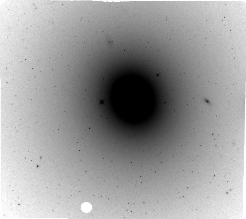
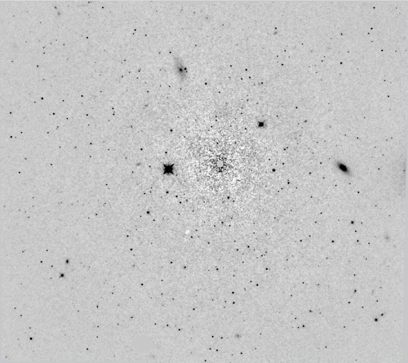
Figure 1.— HST WFC3/IR F160W image of NGC 1399 (top), and the same following galaxy isophotal model and sky subtraction (bottom). The field size is approximately $2\farcm 3\times 2\farcm 1$, and the image is shown at the observed orientation. Pixels flagged as bad in the data quality arrays are zeroed in both panels. The central 1$\farcs$2 of the galaxy was not modeled, and is set to zero in the lower panel.

NGC 1399 has been observed many times before with HST, including several times with the ACS/WFC, allowing us to investigate the optical-IR colors of its GCs. Calibrated observations in F606W from GO-10129 (PI: Puzia) and F475W$\,+\,$F814W from GO-10911 (PI: Blakeslee) were retrieved from the STScI archive and processed with Apsis (Blakeslee et al. 2003) to produce summed, geometrically corrected, cosmic-ray-cleaned images for each bandpass. Reduction of the GO-10911 imaging data is described in more detail by Blakeslee et al. (2010b); the same procedures were applied for the GO-10129 program, which observed nine contiguous fields in F606W. We processed only the four pointings that overlapped with the ACS/WFC images in other bands; three of these pointings overlap with our smaller WFC3/IR field. NGC 1399 was also observed in F475W and F850LP as part of HST program GO-10217 (Jordán et al. 2007); in this case, we used the photometry catalogue produced by that program, as discussed in Section 6.

Throughout this study, we employ the natural photometric systems defined by the instrument bandpasses, rather than converting to the Johnson system. We calibrated the WFC3/IR photometry using the AB zero-point coefficients given by Kalirai et al. (2009) and the ACS photometry using the AB zero points from Sirianni et al. (2005). We corrected for Galactic extinction towards NGC 1399 assuming $E(B{-}V)=0.0125$ mag (Schlegel et al. 1998), the ACS/WFC extinction ratios from Sirianni et al. (2005), and the $H$-band extinction ratio from Schlegel et al. (1998). Table 1 summarizes the observational details of the data sets used in the present study, including in the last column the symbols used to denote magnitudes in the various bandpasses.

3. Object Selection and Photometry

In order to obtain photometric catalogues of GC candidates, we first constructed elliptical isophotal models for the different bandpasses as described in our previous works (e.g., Tonry et al. 1997; Jordan et al. 2004; Blakeslee et al. 2009, 2010b) and used these to subtract the galaxy light. Figure 1 shows our WFC3/IR F160W image of NGC 1399 before and after the galaxy subtraction. The compact sources corresponding to GC candidates, as well as some background galaxies and a few stars, are clearly evident.

We performed object detection using SExtractor (Bertin & Arnouts 1996) with an RMS weight image that included the photon noise and SBF contributions from the subtracted galaxy. The full procedure is described in detail by Jordan et al. (2004, 2007) and Barber DeGraaff et al. (2007). For the most part, we use F814W to define the sample limits because it is a broad bandpass at the red end of the optical spectrum, and the signal-to-noise (S/N) of the data is high, despite the half-orbit integration. For object detection in the ACS images, we required an area of at least four connected pixels above a S/N threshold of two; thus, a minimum S/N of four within the isophotal detection area. The SBF is quite strong in the WFC3 F160W image, and we therefore set the detection threshold higher, requiring a total S/N of at least 6 to avoid spurious detections. Objects were detected and measured in each band separately (rather than “dual image mode”), then the catalogues were matched across bands; this process removes spurious objects from the combined multi-band samples. Figure 2 illustrates the depth of the detection in F814W by plotting the magnitude error within the isophotal area as a function of the SExtractor mag_auto parameter, the estimated total magnitude from SExtractor.

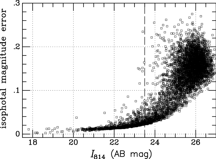
Figure 2.— The error in magnitude for pixels above the isophotal detection threshold is plotted against $I_{814}$ mag_auto values from SExtractor. The magnitudes are on the AB system. The vertical dashed line at $I_{814}=23.5$ mag is drawn somewhat fainter than the mean magnitude (or “turnover”) of the GC luminosity function, which occurs at $I_{814}=23.5$ mag (see text). The median isophotal detection error at $I_{814}=23.5$ is 0.028 mag.

Candidate GCs in NGC 1399 must be nearly point-like objects in the expected magnitude range. Villegas et al. (2010) found that the turnover in the GC luminosity function (GCLF) occurs at $z_{850}=22.802\pm 0.044$, where $z_{850}$ is the total magnitude in F850LP from the ACSFCS. We find in Section 6 that the mean color of the GC candidates is $I_{814}{-}z_{850}\approx 0.3$, where $I_{814}$ is the SExtractor mag_auto value; this would indicate a turnover in F814W of $\sim 23.1$ mag. This is consistent with a magnitude histogram of the GC candidates selected below, although based on the Virgo GCLF and the relative distances of the two clusters, the GCLF turnover would be expected to occur about 0.2 mag fainter. In any case, this is still brighter than the dashed line shown at $I_{814}=23.5$ mag in Figure 2.

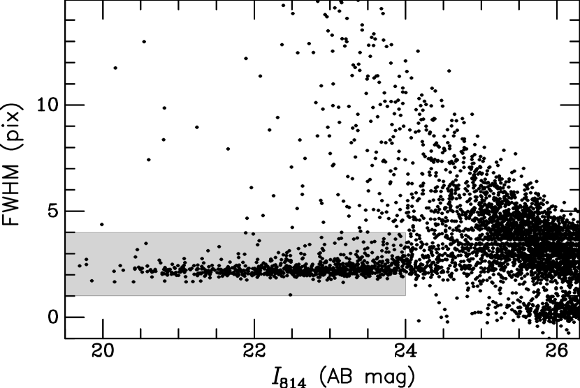
Figure 3.— Full-width half maximum (FWHM) is plotted against $I_{814}$ mag_auto parameter from SExtractor for all objects detected in the ACS/WFC F814W image. The FWHM values are in pixels, at a scale of 0$\farcs$05 pix^-1. The gray shaded region shows the initial selection for GC candidates in this plane. The turnover of the GCLF occurs near $I_{814}\approx 23.2$ mag.

Figure 3 shows the full width at half maximum (FWHM) values measured with SExtractor as a function of $I_{814}$ magnitude. There is a “finger” of compact sources with FWHM $\sim 2$ pix that can be distinguished from the background population down to $I_{814}\approx 24$ mag (shaded region). This is similar to the FWHM of the point spread function, which is about 0$\farcs$09, or 1.8 to 1.9 pix. At the 20 Mpc distance of Fornax, 1″ corresponds to about 96 pc, so the typical GC half-light radius of $r_{h}\approx\,$3 pc corresponds to 0.6 pix for the ACS/WFC. Thus, the GCs are very marginally resolved, and some with smaller $r_{h}$ will be indistinguishable from point sources. For our initial GC candidate selection, we therefore selected all objects in the magnitude range $19.5<I_{814}<23.5$ mag, with $1<\hbox{FWHM}<4$. We also require the candidates to be reasonably round, with ellipticity $<1/3$ (in practice, this rejects very few objects, since they are already required to be compact). In Section 6, where we match our sample against that of the ACSFCS, we confirm that the overwhelming majority of the objects are high-probability GCs.

The catalogs produced by SExtractor include magnitudes measured within many different apertures. In general, we found that the magnitudes of GC candidates measured within the SExtractor 6 pix (diameter) aperture proved to be optimal, in the sense that the scatter between colors was near the minimum, yet the aperture enclosed $\sim 75$% of the total light for point-like objects, thus making a good compromise between statistical and systematic errors (cf. Appendix F of Sirianni et al. 2005). This proved to be the case for both the ACS/WFC and WFC3/IR photometry. Although for the ACS/WFC this aperture corresponds to a radius $r=0\farcs 15$, while for the drizzled WFC3/IR data it is $r=0\farcs 30$, the FWHM of the point spread function (PSF) of WFC3/IR is roughly twice that of ACS/WFC; thus the aperture corrections from Sirianni et al. (2005) and Kalirai et al. (2009) are very similar when the WFC3/IR aperture is twice that of the ACS/WFC aperture in angular units. As a result, the systematic offsets in the aperture colors due to differential PSF effects across bands are relatively small.

Following Jordán et al. (2009), we calculated the color corrections due to differential aperture effects within our apertures ($r=0\farcs 15$ for ACS/WFC; $r=0\farcs 30$ for WFC3/IR) for a typical GC (King model with $r_{h}=3$ pc and concentration $c=1.5$) convolved with the PSF. For $g_{475}{-}I_{814}$, $V_{606}{-}I_{814}$, $V_{606}{-}H_{160}$, and $I_{814}{-}H_{160}$, the estimated corrections are: $+0.02$, $+0.01$, $-0.01$, and $-0.02$ mag, respectively. Since these offsets are small, systematic, and systematically uncertain at the $\sim 0.02$ mag level, we have not applied them to our colors for this analysis, but simply note that such offsets would be expected for some external comparisons. The conclusions of this work would not change. In contrast, the corresponding corrections would be $\sim 0.1$ mag for colors involving $z_{850}$, since the PSF is significantly broader in that band; however, in that case (see Section 6), we use the ACSFCS photometry, for which the colors have been converted to the infinite-aperture values assuming the King model profile for a typical GC convolved with the PSF (see Jordan et al. 2009).

4. Color Distributions

NGC 1399 was one of the first galaxies suggested to show evidence for bimodality in its GC metal distribution, based on Washington system photometry (Ostrov et al. 1993), although there was no clear separation between the proposed components in the color distribution of that early sample. The bimodality result, again based on photometric colors, was more evident for some other galaxies (e.g., Zepf & Ashman 1993). It is now clear that the situation in NGC 1399 is more complex. Color bimodality is present in the system, but not for all subsamples, and we first address this issue.

Figure 4.— Optical color-magnitude diagrams for GC candidates in NGC 1399 from ACS/WFC imaging. Dashed horizontal lines indicate the range over which the color histograms are significantly bimodal, and the vertical lines indicate the peaks in the color distributions for this magnitude range. The brightest GCs, more than $\sim\,$2 mag above the turnover, do not exhibit distinct bimodality because NGC 1399 is a strong “blue tilt” galaxy.

4.1. Optical Colors by Magnitude

Dirsch et al. (2003) discussed the “striking” difference in the color distribution of NGC 1399’s brightest GCs compared to those within $\lesssim 2$ mag of the GCLF turnover, based on wide-field CTIO 4 m Mosaic imaging extending to $\sim 20\arcmin$. The GCs in their brightest magnitude bin followed a unimodal color distribution peaking at $C{-}T_{1}\approx 1.5$ in the Washington system, whereas GCs in the next two magnitude bins exhibited a clearly bimodal color distribution with the “gap” occurring near the same $C{-}T_{1}\approx 1.5$ color. This confirmed the earlier result based on a smaller sample by Ostrov et al. (1998) that the brightest $\sim 1$ mag of the GC population had a broad color distribution, with a mean color similar to the location of the gap in the distribution of the fainter GCs. Dirsch et al. also found that the red peak was only prominent at $r\lesssim 9\arcmin$, and is more of a red tail at larger radii. Bassino et al. (2006) analyzed two additional Mosaic fields to extend the areal coverage of NGC 1399 GC system even further, and found results similar to those of Dirsch et al. (2003).

Figure 4 shows our $g_{475}{-}I_{814}$ and $V_{606}{-}I_{814}$ versus $I_{814}$ color-magnitude diagrams (CMDs) for GC candidates selected in $I_{814}$, as described above, and matched with objects detected in the GO-10911 $g_{475}$ data (taken at the same pointing and within the same orbit as $I_{814}$) and, separately, with objects detected in $V_{606}$ from the multi-pointing GO-10129 observations. The colors are measured within the adopted $r=3$ pix aperture, and we only consider objects with color errors $<0.2$ mag for this aperture. Many large galaxies exhibit a “blue tilt” in their CMDs, a tendency for GCs in the blue peak to become redder at higher luminosities, sometimes merging together with the red component (Harris et al. 2006; Mieske et al. 2006; Strader et al. 2006; Peng et al. 2009). In this sense, NGC 1399 is a very strong “blue tilt galaxy,” since the two color components merge for the brightest GCs (Dirsch et al. 2003; Mieske et al. 2010). However, Forte et al. (2007) find that for fainter GCs, in the luminosity range where the distribution is clearly bimodal, there is no significant slope in the color of the blue peak with magnitude. This is consistent with models in which the tilt is due to self-enrichment and requires some minimum GC mass threshold (Bailin & Harris 2009). Blakeslee et al. (2010a) showed that a simple mass-metallicity relation, combined with a nonlinear color-metallicity transformation, can produce bimodal color distributions with a blue tilt in GC populations with broad unimodal metallicity distributions. In Figure 4, the horizontal lines enclose the magnitude range in NGC 1399 where the bimodality is most evident, and the vertical lines show the approximate locations of the peaks, found below. The tilting of the blue GCs towards the red at $I_{814}<21.5$ is clear.

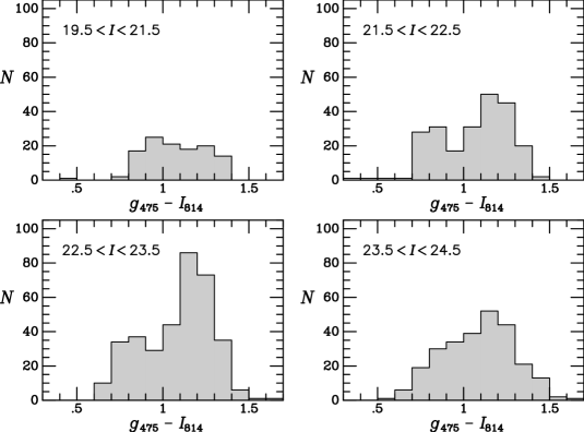
Figure 5.— Histograms of $g_{475}{-}I_{814}$ colors for different $I_{814}$ magnitude ranges.

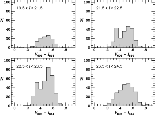
Figure 6.— Histograms of $V_{606}{-}I_{814}$ colors for different $I_{814}$ magnitude ranges.

Figures 5 and 6 display $g_{475}{-}I_{814}$ and $V_{606}{-}I_{814}$ histograms for GC candidates in several different $I_{814}$ magnitude ranges (note that there are only four brighter than $I_{814}{\,=\,}20$). In both cases, the appearance of bimodality is greatest within the $21.5<I_{814}<22.5$ and $22.5<I_{814}<23.5$ magnitude ranges. Although the $g_{475}{-}I_{814}$ colors in the brightest magnitude range of Figure 5 appear somewhat bimodal, the blue “peak” in this bright range coincides with the “gap” at $g_{475}{-}I_{814}\approx 0.95$ in the color histograms of the fainter GCs. The situation is similar in Figure 6, although in that case, the histogram of the brightest GCs is essentially a broad red distribution that encompasses the gap at $V_{606}{-}I_{814}=0.4$ for the fainter GCs.

Thus, although the Dirsch et al. (2003) and Bassino et al. (2006) studies covered a much larger area than our HST data, we find the same lack of obvious bimodality in the color distribution of the brightest GCs. Our principal goal here is to examine the optical-IR colors for GCs that define a distinctly bimodal distribution in purely optical colors. This provides a simple, fairly direct test of whether the colors linearly trace metallicity and reflect true bimodality in the underlying distribution. In the following section, we therefore compare the purely optical and optical-IR color distributions over the $21.5<I_{814}<23.5$ magnitude range where the optical bimodality is strongest.

Figure 7.— Optical-IR color-magnitude diagrams. The dashed horizontal lines are shown to facilitate comparison with the $I_{814}$ region enclosed by similar lines in Figure 4; they have been shifted by the mean $I_{814}{-}H_{160}$ color of 0.70 mag.

4.2. Optical-IR Color Distributions

For comparison to Figure 4, we show the $V_{606}{-}H_{160}$ and $I_{814}{-}H_{160}$ versus $H_{160}$ CMDs in Figure 7. The colors are measured within apertures of $r{\,=\,}3$ pix, as described in Section 3. Again, only objects with color errors $<0.2$ mag are shown. The horizontal lines here are the equivalent of those shown in Figure 4, but shifted by the mean $\langle I_{814}{-}H_{160}\rangle=0.70\pm 0.01$ mag. They are merely for comparison to the previous CMDs, not to select a magnitude range with the most bimodality. Any bimodality in these CMDs is much less evident.

Figure 8 shows the binned $g_{475}{-}I_{814}$, $V_{606}{-}I_{814}$, $I_{814}{-}H_{160}$, and $V_{606}{-}H_{160}$ color distributions, along with smooth density estimates constructed with a Gaussian kernel. The colors involving $I_{814}$ use the magnitude range selected above, while for $V_{606}{-}H_{160}$, we use $22<V_{606}<24$, as the mean $V_{606}{-}I_{814}$ color is 0.49 mag. We did this for convenience because the pairs of bandpasses were matched separately at this stage; in Section 6, we examine the colors of a single merged sample. In any case, the selection on either $I_{814}$ or $V_{606}$ makes no difference to the conclusions here. The $g_{475}{-}I_{814}$ and $V_{606}{-}I_{814}$ color distributions appear strongly bimodal, both having two distinct peaks with the red peak containing roughly 2/3 of the GC population. The predominance of red GCs occurs because the HST fields cover a relatively small central area, and the NGC 1399 GC system has a radial color gradient. The $I_{814}{-}H_{160}$ and $V_{606}{-}H_{160}$ distributions appear quite similar to each other: unlike in the optical colors, there are no well-separated peaks, although neither do they appear to be simple Gaussians. The $V_{606}{-}H_{160}$ distribution shows some evidence for a blue component; this is understandable because $I_{814}{-}H_{160}$ is sharply peaked (though, again, not symmetric), while $V_{606}{-}I_{814}$ is bimodal, so $V_{606}{-}H_{160}$ would be expected to show some bimodality.

We have used the GMM code (“Gaussian Mixture Modeling”) of Muratov & Gnedin (2010) to quantify the above qualitative impressions. These authors provide a detailed discussion of the issues and pitfalls inherent in bimodality tests. They note that Gaussian mixture modeling such as GMM or KMM (Ashman et al. 1994), by itself, is more a test of Gaussianity than unimodality. As observed by many authors, unimodal but skewed distributions will strongly favor a double Gaussian model, even if there is no true bimodality in the distribution. To address this point, they emphasize the importance of the kurtosis, stating that “$\hbox{\it kurt}<0$ is a necessary but not sufficient condition of bimodality.” This is true because the sum of two populations with different means is necessarily broader than a single population; therefore, in the case of Gaussians, which have $\hbox{\it kurt}=0$, the kurtosis must be negative for a valid double Gaussian decomposition. In addition, following Ashman et al. (1994), Muratov & Gnedin define the quantity $D$ as the separation between the means of the component Gaussians relative to their widths; they state that Gaussian splits that appear significant based on the $p$ value but have $D<2$ are “not meaningful,” in the sense that they do not demonstrate clear bimodality, but non-Gaussianity.

Table 2 presents our GMM analysis results; the errors on the tabulated quantities come from the bootstrap resampling done in the GMM code. Note that the analysis is independent of any binning. The full $g_{475}{-}I_{814}$ sample for the $21.5<I_{814}<23.5$ magnitude range contains 584 objects and strongly prefers a double Gaussian model with peaks at $0.83\pm 0.02$ and $1.19\pm 0.01$ mag. (We remind the reader that the small offsets for aperture corrections, as given in Section 3 should be applied for external comparisons.) About 70% of the GC candidates are assigned to the red component. The kurtosis is negative, and $D$ is significantly above 2, confirming a valid bimodal Gaussian model. We therefore assign a “Y” in the last column of Table 2 to indicate the affirmative on the question of bimodality. However, because the $g_{475}{-}I_{814}$ distribution has a few outliers in tails, and mixture modeling codes are generally sensitive to extended tails, we ran another test after restricting the range to $0.6<g_{475}{-}I_{814}<1.5$. The results, given in the second row of Table 2, are very similar to prior run, but with the kurtosis being even more negative and the model uncertainties slightly reduced. The situation is very similar for $V_{606}{-}I_{814}$, which favors a well-separated double Gaussian model with peaks at $0.34\pm 0.01$ and $0.54\pm 0.01$ mag, and $74\pm 3$% of the GCs assigned to the red peak. Again, we answer “Y” to the question of bimodality.

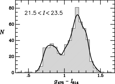
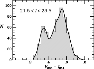
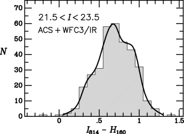
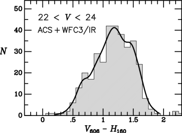
Figure 8.— Histograms of $g_{475}{-}I_{814}$, $V_{606}{-}I_{814}$, $I_{814}{-}H_{160}$, and $V_{606}{-}H_{160}$ colors for all matched GC candidates in the specified magnitude ranges and with color errors less than 0.2 mag.

Consistent with the visual impression, the GMM code finds that the $I_{814}{-}H_{160}$ distribution is not bimodal. When run on the full distribution in Figure 8, the few objects in the tails result in a positive kurtosis and virtually all of the objects are assigned to the red peak. When we restrict the color range to $0.1<I_{814}{-}H_{160}<1.3$, the kurtosis becomes negative as required, but the $p$ value of the double Gaussian model is not significant, and the fraction of objects assigned to the second component is consistent with zero.

For $V_{606}{-}H_{160}$, the situation is a bit more nuanced. For GC candidates in the broad color range $0<V_{606}{-}H_{160}<2$, the kurtosis is negative, and the $p$ value of 0.01 is marginally significant, but the separation $D$ is not meaningful. Moreover, the weakly favored decomposition has only $39\pm 22$% of the GCs in the red peak, as compared to $\sim 70$% for the optical decomposition. If we remove the two bluest outliers, the $p$ value becomes slightly less significant, but now $D$ is marginally above 2, and the fraction of objects in the second (red) peak is consistent with that found in the optical, although it is also consistent with 100% at the 2-$\sigma$ level. We therefore answer an uncertain “Y?” to the question of bimodality here, consistent with unimodality in $I_{814}{-}H_{160}$ but bimodality in $V_{606}{-}I_{814}$.

As another test of the bimodality in the color distributions, we ran the “Dip” test (Hartigan & Hartigan 1985) supplied with GMM, which nonparametrically measures the significance of any gaps, or “dips,” in a distribution. Since the Dip test is insensitive to the assumption of Gaussianity, it is much more robust, but as discussed by Muratov & Gnedin, the returned significance levels are much lower than for the parametric GMM analysis. Probabilities above $\sim 50$% may be taken as indicative of likely bimodality. From this test, we found that the probability for the most significant gaps in the $g_{475}{-}I_{814}$, $V_{606}{-}I_{814}$, $I_{814}{-}H_{160}$, and $V_{606}{-}H_{160}$ distributions to be real were 75%, 97%, 4%, and 22%.

Overall, we confirm that the $g_{475}{-}I_{814}$ and $V_{606}{-}I_{814}$ distributions for GCs in NGC 1399 are strongly bimodal, with consistent proportions of red and blue GCs, when the brightest GCs are excluded. The $I_{814}{-}H_{160}$ distribution is not significantly bimodal, but there is marginal evidence for bimodality in $V_{606}{-}H_{160}$ consistent with the proportions found for $g_{475}{-}I_{814}$ and $V_{606}{-}I_{814}$. This is understandable if the optical color bimodality is partly the result of a changing horizontal branch morphology, since the colors involving bluer bandpasses would be more affected by the behavior of the hot horizontal branch stars, whereas colors such as $I_{814}{-}H_{160}$ would not. Thus, some evidence for bimodality in $V_{606}{-}H_{160}$ would be expected, but weaker than that found for $V_{606}{-}I_{814}$ (Cantiello & Blakeslee 2007).

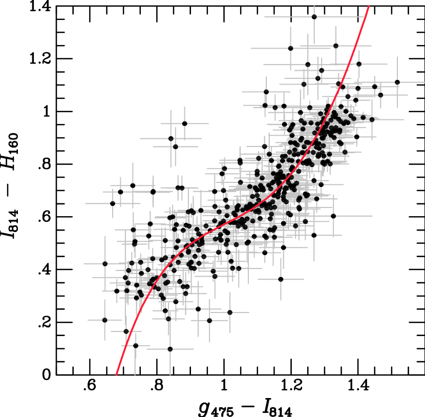
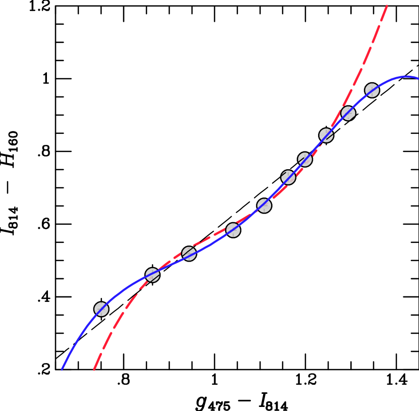
Figure 9.— The ACS+WFC3/IR $I_{814}{-}H_{160}$ versus $g_{475}{-}I_{814}$ color-color plots. In the left panel, the invidual matched GC candidates are shown, with error bars estimated from the RMS images mentioned in Section 3. The red curve represents a 4th-order robust polynomial fit with coefficients given in the text. The right panel shows the median values within ten bins (40 objects per bin) ordered by $g_{475}{-}I_{814}$. We also plot the same polynomial fit as in the left panel (red dashed curve), a 4th-order polynomial fit to the median points (blue curve), and a linear fit to these points (black dashed line). Error bars on the points are plotted, but in most cases they are smaller than the point size. The plot scale is expanded in the right panel to clarify the differences between the fits.

5. Color-Color Curvature

The broadest baseline color-color combination we have available for investigating stellar population issues is $g_{475}{-}I_{814}$ versus $I_{814}{-}H_{160}$. These color indices span factors of 1.7–2.0 in wavelength. The $g_{475}{-}I_{814}$ index for GCs is affected by the properties of stars near the main sequence turnoff, on the horizontal branch, and on the giant branch. It is therefore sensitive to metallicity, age, and any other parameters (e.g., helium) that affect the temperature of the main sequence and the morphology of the horizontal branch. By comparison, the $V_{606}{-}I_{814}$ index spans a much smaller factor (1.3) in wavelength, and is less sensitive than $g_{475}{-}I_{814}$ to features such as the blue horizontal branch. As discussed in the Introduction, colors such as $I_{814}{-}H_{160}$ are mainly sensitive to the temperature of the giant branch, which is controlled by metallicity with very little age dependence. Colors such as $g_{475}{-}H_{160}$ and $V_{606}{-}H_{160}$ are also sensitive to giant branch temperature, but they complicate the metallicity dependence with additional sensitivity to the main sequence turnoff and horizontal branch. We therefore concentrate now on the relation between $g_{475}{-}I_{814}$ and $I_{814}{-}H_{160}$.

Figure 9 (left panel) plots $I_{814}{-}H_{160}$ as a function of $g_{475}{-}I_{814}$ for 401 NGC 1399 GC candidates in our combined ACS-WFC3 data set with $19.5<I_{814}<23.5$ and $0.5<g_{475}{-}I_{814}<1.6$. The corresponding data are listed in Table 3. Although we deal throughout this work with aperture colors within a 3-pixel radius, in order to facilitate external comparisons, the last two columns of Table 3 provide colors that have been corrected for differential aperture effects, assuming the corrections for a typical GC, as given in Section 3. Since we are interested here in the relationship between these color indices, rather than simply the presence or absence of bimodality, we improve the statistics by including the GCs from the brightest magnitude range in Figure 5, increasing the sample by 17%. The relation appears nonlinear. The plotted curve represents a quartic (4th order) polynomial, which has been fitted to the data using robust orthogonal regression (Jefferys et al. 1988). This approach minimizes the residuals in the direction orthogonal to the fitted relation, and it is appropriate here because of the significant observational scatter in both coordinates. The fitted coefficients are given by

$$\hbox{$I_{814}{-}H_{160}$}\;=\;-14.54\,+\,49.23x\,-\,59.02x^{2}\,+\,30.14x^{3}$$

$$\,-\;5.24x^{4}\,,$$ (1)

where $x\equiv(g_{475}{-}I_{814})$. Several of the objects appear discrepant with respect to this relation: these may be due to contamination in the sample from Galactic stars and/or background galaxies, or to real stellar population variations. In particular, objects that lie above or to the left of the relation could be young clusters, or they may have extreme horizontal branches. Despite some outliers, there is a tight locus of objects that define the curved sequence in color-color space traced by the above fit.

To further illustrate the curvature, we have binned the data by $g_{475}{-}I_{814}$ into 10 groups of 40 objects, and we plot the median values of the colors within the bins in the right panel of Figure 9. The polynomial fit from the left panel is plotted again, as well as linear and quartic fits to the binned data. The deviation from a linear relation is highly significant. If we use the scatter to estimate the errors ($\sigma/\sqrt{N}$) in the medians, the value of the reduced $\chi^{2}_{\nu}$ is 2.7 for the linear fit, and 0.1 for the quartic fit. Thus, the linear fit is strongly rejected. The low value of $\chi^{2}_{\nu}$ for the quartic fit probably indicates that the uncertainties in the medians have been overestimated, most likely because the small fraction of outliers make the scatter estimate too high. This also suggests that $\chi^{2}_{\nu}$ should be larger than 2.7 for the linear fit. The 4th order model closely traces the curvature of the binned points; adding another term to the polynomial does not reduce $\chi^{2}_{\nu}$ further. The polynomial fits to the binned and unbinned data diverge near the endpoints because of the lack of constraints, but they agree well over the $\sim\,$0.8–1.3 color range.

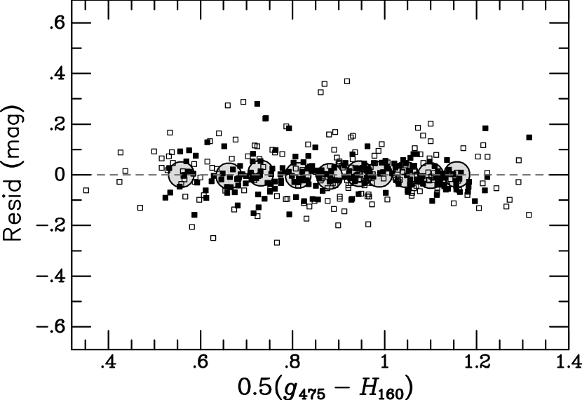
Figure 10.— Color-color fit residuals are plotted as a function of $0.5\times(g_{475}{-}H_{160})$, which corresponds to the mean of $g_{475}{-}I_{814}$ and $I_{814}{-}H_{160}$. We use this mean for the horizontal axis because it is approximately orthogonal to the residuals that were minimized in the robust regression fitting (see text). Square symbols show the orthogonal residuals for individual GC candidates with respect to the curve in the left panel of Fig. 9. Filled squares are used for objects with $I_{814}<22.5$, while open squares are used for objects with $22.5\leq I_{814}<23.5$. The large circles indicate the quartic fit residuals for the median points shown in the right panel of Fig. 9.

Figure 10 shows the fit residuals as a function of the mean of the $g_{475}{-}I_{814}$ and $I_{814}{-}H_{160}$ colors, which corresponds to half of the $g_{475}{-}H_{160}$ color. Since the color-color relation has an average slope of about one (the linear fit in Figure 9 has slope $1.01\pm 0.06$), this mean color is, to a good approximation, proportional to the distance along the relation (and therefore in the direction orthogonal to the residuals). The small squares in this figure represent individual GC candidates, and their residuals are with respect to the fit given in equation (1). Open squares are used for the faintest magnitude of GC candidates included in the fitting, while solid squares are used for brighter objects. The fainter objects scatter more, but otherwise do not differ systematically from the brighter ones. The large circles in Figure 10 show the residuals for the median-filtered points with respect to the quartic fit for these points plotted as a solid curve in the right panel of Figure 9. In this case, the median values have very little scatter, and the fit is essentially identical regardless of whether orthogonal regression or a simple least-squares approach (minimizing residuals in $I_{814}{-}H_{160}$) is used. From Figure 10, we conclude that the form of the color-color relation is well approximated by a quartic polynomial over a range in $g_{475}{-}H_{160}$ from $\sim\,$1.3 to $\sim\,$2.2 mag, which corresponds approximately to the $0.8\lesssim g_{475}{-}I_{814}\lesssim 1.3$ mag range quoted above.

We emphasize that not only is the relation between $g_{475}{-}I_{814}$ and $I_{814}{-}H_{160}$ nonlinear, but the slope attains a local minimum within the color range where it is particularly well constrained. In fact, the inflection point of the quartic fit to the unbinned data occurs at $g_{475}{-}I_{814}=1.002$, which corresponds closely to the dip in the $g_{475}{-}I_{814}$ color distribution in Figure 8. If $I_{814}{-}H_{160}$ is a good, relatively simple, indicator of metallicity, in line with theoretical expectations, then this type of “wavy” or inflected relation could produce double-peaked optical color histograms from metallicity distributions that have a very different form. The metallicity distribution does not need to be unimodal or even symmetric; chemical enrichment scenarios tend to produce asymmetric distributions (see Yoon et al. 2011b for a detailed discussion of this issue). We address the metallicities briefly in the following section.

The observed wavy relation between $g_{475}{-}I_{814}$ and $I_{814}{-}H_{160}$ accounts for the marked difference between the purely optical and optical-IR color distributions found in Figure 8. The significance of the curvature demonstrates that the apparent disparity was not the result of underestimated photometric errors obscuring bimodality in $I_{814}{-}H_{160}$.

6. ACSFCS Comparison: Implications for Metallicity

The ACSFCS (Jordán et al. 2007) is a survey with ACS in the F475W and F850LP bands of 43 early-type Fornax cluster galaxies. All objects with colors and magnitudes consistent with GCs in the program galaxies were fitted with King (1966) models using the methodology of Jordán et al. (2005) to derive half-light radii $r_{h}$ and total magnitudes. As described in Jordán et al. (2009), objects with colors in the range $0.5<g_{475}{-}z_{850}<1.9$ and radii $0.75<r_{h}<10$ pc were assigned probabilities $p_{\rm GC}$ of being GCs based on their $z_{850}$ magnitudes and half-light radii, as compared with those found for objects in background fields. Those with $p_{\rm GC}>0.5$ were accepted as likely GCs. For the $g_{475}{-}z_{850}$ colors considered in this section, we used the NGC 1399 photometric catalogue produced as described in Jordán et al. (2009) and already used in several ACSFCS publications (Masters et al. 2010; Mieske et al. 2010; Villegas et al. 2010; Liu et al. 2011).

We used the object positions to match the ACSFCS photometry for NGC 1399 with our $g_{475}$, $I_{814}$, and $H_{160}$ measurements. We keep high probability GCs with $p_{\rm GC}\geq 0.9$ (in practice, there was only one matched object with $0.5<p_{\rm GC}<0.9$). This merged data set provides two important benefits. First, the probabilistic selection based on $r_{h}$ and $z_{850}$ should remove most of the remaining contaminants in our sample. Second, the ACS $g_{475}{-}z_{850}$ colors have been calibrated empirically against metallicity. Although the throughput for objects with GC spectra is about twice as high in F814W as in F850LP, allowing more precise color measurements with $I_{814}$ for a given exposure time, the longer baseline afforded by $z_{850}$ improves the metallicity sensitivity (Côté et al. 2004). Peng et al. (2006) found that the relation between $[\hbox{Fe/H}]$ and $g_{475}{-}z_{850}$ was not adequately described by a linear fit; they used a broken linear model with a shallower slope for $g_{475}{-}z_{850}>1.05$. This was adequate over the range $g_{475}{-}z_{850}=0.7$–1.4, but under-predicted the spectroscopic metallicities of M87 and M49 GCs in the 1.4–1.6 color range. Additional curvature was needed to match these. To accommodate the measured metallicities of these redder GCs, Blakeslee et al. (2010a) used a polynomial fit that followed the data over the full 0.7–1.6 range in $g_{475}{-}z_{850}$. This empirical calibration provides us with some handle on the metallicities for our sample.

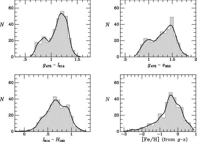
Figure 11.— Histograms of $g_{475}{-}I_{814}$, $g_{475}{-}z_{850}$, and $I_{814}{-}H_{160}$ colors, along with $[\hbox{Fe/H}]$ values inferred from ACSFCS $g_{475}{-}z_{850}$ data (see text), are plotted for GC candidates identified in the ACS Fornax Cluster Survey.

Figure 11 shows the color and estimated metallicity histograms for our sample of ACS+WFC3 data after merging with the ACSFCS dataset. Again we use the $21.5<I_{814}<23.5$ magnitude range for the histograms to select the regime of optical color bimodality. After the merging with ACSFCS, there was one object at $g_{475}{-}I_{814}=0.45$ mag, whereas all the others were in the 0.64–1.52 range; we removed this single outlier in $g_{475}{-}I_{814}$ color. In contrast to the approach in Figure 8, the exact same 322 high-probability GCs are represented in all of the color histograms in Figure 11. For uniformity, we have used the same binsize of 0.07 mag for all the colors. The change in binning is mainly responsible for the different appearance of the $I_{814}{-}H_{160}$ histograms in Figures 8 and 11, but the kernel density curves reflect the same features.

As described above, the metallicity histogram in the lower right of Figure 11 is based on the polynomial fit by Blakeslee et al. (2010a) to the Peng et al. (2006) data. We use this polynomial transformation only for objects with $g_{475}{-}z_{850}<1.6$ mag, since it is not constrained beyond this; objects with redder $g_{475}{-}z_{850}$ colors (7.5% of our merged sample) are likely affected by observational scatter. Thus, there are fewer objects in the $[\hbox{Fe/H}]$ histogram, and the truncation at $[\hbox{Fe/H}]=0.76$ dex is artificial. However, the peak at $[\hbox{Fe/H}]\approx-0.3$ dex, and the long tail to lower metallicities, accurately reflect the $g_{475}{-}z_{850}$ distribution combined with the empirical metallicity calibration.

Table 4 summarizes the GMM results for this merged sample. For the $g_{475}{-}I_{814}$ distribution, we again find a significant preference for a double Gaussian model, with peaks at $0.84\pm 0.02$ and $1.20\pm 0.01$ mag and $73\pm 5\%$ of the objects in the red component. The result is similar for $g_{475}{-}z_{850}$, with peaks at $0.98\pm 0.04$ and $1.41\pm 0.01$ mag and $72\pm 7\%$ in the red component. When the analysis is run on the full $I_{814}{-}H_{160}$ sample, we find $\hbox{\it kurt}>0$, $D<2$, and $p\gtrsim 0.05$; thus, no significant evidence for a bimodal model. However, no outliers have been trimmed from the $I_{814}{-}H_{160}$ distribution; if we remove the two objects with $I_{814}{-}H_{160}<0$, then the fourth row of Table 4 shows $\hbox{\it kurt}<0$, as required for significant Gaussian bimodality, but the $p$ value increases to 0.055, and $D$ is unchanged, except in the uncertainty. If we trim the outliers more aggressively, restricting the range to $0.2<I_{814}{-}H_{160}<1.2$, then kurt decreases further, and the separation between the best-fit peaks is now a marginally significant $D=2.0\pm 0.3$, but $p$ increases to 0.062 (significance less than 2$\sigma$). Moreover, the preferred breakdown has $24\pm 28\%$ of the objects in the red component (before the trimming, the red percentage was even lower). This red fraction is consistent with zero; however, if it were interpreted as real, then this would indicate a “different bimodality” than that found for the optical colors, where $\sim\,$73% of the objects are in the red peak. Thus, the preferred optical and optical-IR bimodalities could not both reflect a common, more fundamental bimodality in metallicity.

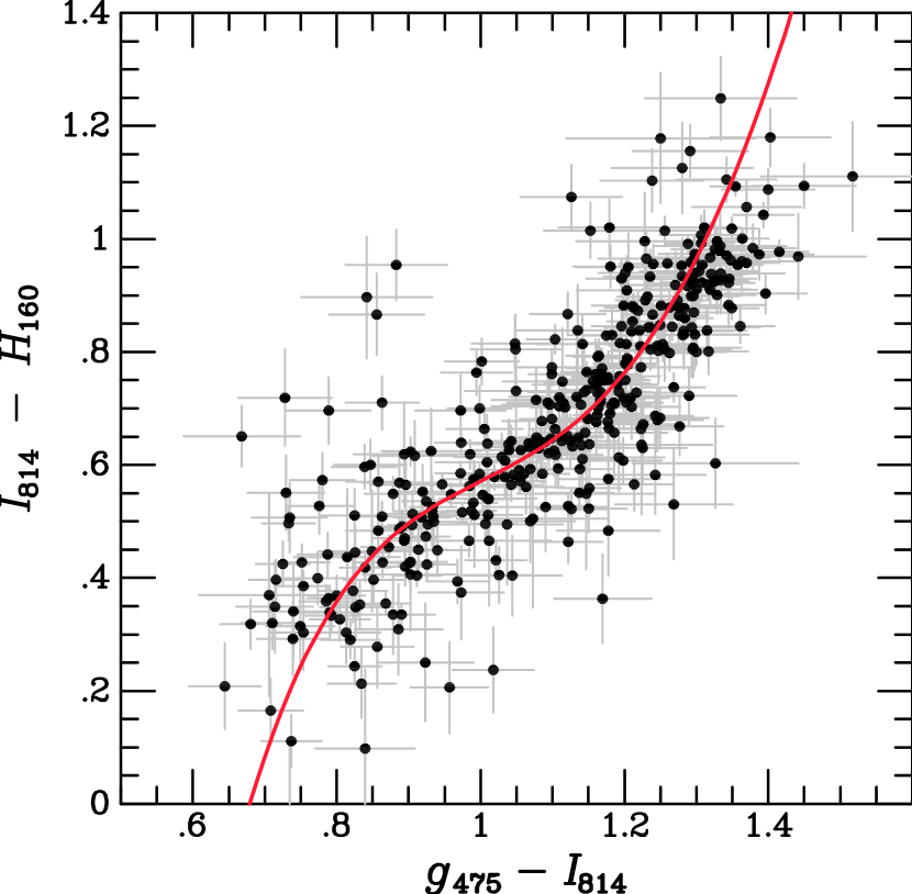
Figure 12.— Similar to the left panel of Figure 9, but here shown for the merged sample of high-probability GC candidates identified in the ACSFCS. The $g_{475}{-}z_{850}$ measurements are from the ACSFCS.

We also experimented with the GMM analysis for the $[\hbox{Fe/H}]$ distribution derived from the $g_{475}{-}z_{850}$ colors. For the full sample, the kurtosis is significantly above zero, and the code wants to fit a primary peak with 80% of the objects, then use another broad Gaussian for the blue tail. This reflects the obvious lack of Gaussianity. If we aggressively trim the blue tail, removing objects with $[\hbox{Fe/H}]<-1.9$, then we find $\hbox{\it kurt}<0$, $p=0.002$, and $D>2$. However, the fraction of objects in the main peak is then $0.917\pm 0.084$, consistent with 100%. More to the point, this procedure of removing members of a continuous extended distribution (rather than outliers), is not statistically valid; we have done so only for illustration. The metallicities for NGC 1399 GCs derived from the (bimodal) $g_{475}{-}z_{850}$ colors and empirical calibration define a continuous distribution with a peak at $\sim\,-$0.3 dex and an extended blue tail. The form of the high-metallicity end is unknown, but it is unlikely to extend much beyond the limit imposed here by the calibration.

Figure 12 plots $I_{814}{-}H_{160}$ versus $g_{475}{-}I_{814}$ and $g_{475}{-}z_{850}$ for the merged sample. This includes 385 objects with $19.5<I_{814}<23.5$; thus, the merging with ACSFCS removed only 16 objects, or 4% of the sample. The resulting plot for $g_{475}{-}I_{814}$ is essentially identical to that in Figure 9. The robust orthogonal regression insured that the rejected objects (possible contaminants) did not strongly affect the fit. To illustrate the consistency between the two relations in Figure 12, we have not independently fitted the relation for the ACSFCS $g_{475}{-}z_{850}$ colors, but simply transformed the fit for $g_{475}{-}I_{814}$ aperture colors according to the linear relation we find for the data:

$$(g_{475}{-}I_{814})_{\rm r{=}3p}\;=\;0.13\,+\,0.75(g_{475}{-}z_{850})_{\rm ACSFCS}\,.$$ (2)

It is not surprising that the relations between $I_{814}{-}H_{160}$ and these two optical colors would be very similar, since they have the same blue bandpass, and there is substantial wavelength overlap of the red bandpasses. We note however that the $g_{475}$ measurements are from independent data sets, one taken at the same time and orientation as the $z_{850}$ data in HST Cycle 13, and the other taken with the $I_{814}$ data in Cycle 15.

The merged sample analyzed here is nearly 5 times larger than previous optical-IR color studies of GCs with HST, and has significantly better precision than previous ground-based studies. Clearly, even larger, high-quality optical-IR samples are needed to explore higher-order features of the color-color relations presented here. Deep spectroscopy of representative portions of the photometric samples is also essential for more detailed constraints on the underlying metallicity distributions. We are currently analyzing the full sample of 16 galaxies from our WFC3/IR program, all of which have existing ACS $g_{475}{-}z_{850}$ data. The results from that larger sample will allow us to test the conclusions from the present study.

7. Discussion and Conclusions

In this study, we have combined ACS and WFC3/IR photometry to examine optical and optical-IR color distributions and color-color relations for $\sim\,$400 GCs in NGC 1399, the central giant elliptical in Fornax. Consistent with previous wide-field studies (e.g., Dirsch et al. 2003), we find that the brightest GCs (about 2-3 mag brighter than the GCLF turnover) in NGC 1399 have a broad red distribution in optical colors. Fainter than this, the optical colors become strongly bimodal, with $\sim 70\%$ of the GCs in the red component. Any bimodality in the optical-IR colors is much less clear; for $I_{814}{-}H_{160}$, the preferred relative proportion of red and blue GCs also differs from in the optical.

In addition, the relation between pure optical and optical-IR color is significantly nonlinear. The slope of the dependence of $I_{814}{-}H_{160}$ on $g_{475}{-}I_{814}$ has a local minimum near $g_{475}{-}I_{814}\approx 1$ (the polynomial fit has a true inflection point here), corresponding approximately to the dip in the $g_{475}{-}I_{814}$ distribution; the result is similar for $g_{475}{-}z_{850}$. Since GC color is mainly determined by metallicity, at least one of the color-metallicity relations must also be significantly nonlinear. Such nonlinearities can produce bimodal color distributions even when the metallicity distribution lacks any clear bimodality (Richtler 2006; Yoon et al. 2006; Cantiello & Blakeslee 2007). The main requirement is that the slope in metallicity as a function of color must have a local minimum near the mid-range of the color distribution (for additional discussion, see Blakeslee et al. 2010a). Such “wavy” nonlinearity for optical colors is predicted by some stellar population models (Lee et al. 2002; Yoon et al. 2006, 2011a,b; Cantiello & Blakeslee 2007), largely as a result of the behavior of the horizontal branch (still imperfectly modeled).

Further evidence for nonlinearity comes from the observed relation of $g_{475}{-}z_{850}$ colors of GCs with respect to spectroscopically estimated metallicities (Peng et al. 2006). We have used a smooth fit to this relation, along with $g_{475}{-}z_{850}$ colors from the ACSFCS, to estimate metallicities for the GCs in our sample. Matching with the ACSFCS, which used an independent, probabilistic method for selecting GCs, also confirms that the level of contamination in our sample is quite small. The metallicities derived from the $g_{475}{-}z_{850}$ colors follow a continuous distribution that peaks at $\sim-0.3$ dex and extends in a low-metallicity tail to $[\hbox{Fe/H}]\approx-3$. Because of the limited range of the calibration, the form of the high-metallicity end remains uncertain, but it cannot have the same long extent in logarithmic space as the low-metallicity tail. This skewed distribution, based on the empirical calibration, closely resembles the GC metallicity distributions derived by Yoon et al. (2011b) using their model color-metallicity relations. As these authors have pointed out, the resulting distributions are in much better agreement with those of the halo stars in the same early-type galaxies.

The relative importance of the form of the color-metallicity relation on the one hand, and structure in the underlying metallicity distribution on the other hand, remains an unresolved question, at least in the minds of many. One argument against the importance of nonlinear color-metallicity relations in extragalactic GC populations comes from the bimodal GC metallicity distribution in the Milky Way Galaxy (e.g., Zinn 1985). However, it is unclear if the GC system of the Milky Way would be recognized as bimodal to an outside observer, given the necessity of avoiding disk contamination when selecting GCs in spirals. For instance, Zepf & Ashman (1993) show that the metallicity distribution of the Milky Way halo GCs, the subpopulation that they considered relevant for comparison with elliptical galaxies, is unimodal. Furthermore, the generalization of the Milky Way’s properties to galaxies such as NGC 1399, which has $\sim\,$40 times as many GCs and must have had a much more chaotic interaction history than a spiral galaxy in a low-density group, is uncertain. It is clear that the metallicity peaks in the Milky Way do not correspond with those derived for giant ellipticals based on linear transformations of optical colors (e.g., Zepf & Ashman 1993; Gebhardt & Kissler-Patig 1999; Peng et al. 2006).

Several other large, nearby galaxies possess extensive GC systems that are probably better analogues to those of giant ellipticals. The nearest of these is M31, with roughly 500 confirmed GCs (Huxor et al. 2011). Based on high-quality spectroscopic metallicities for 322 M31 GCs (twice as many as in the whole of the Milky Way), Caldwell et al. (2011) find that the metallicity distribution does not evince clear bimodality, “in strong distinction with the bimodal Galactic globular distribution.” Instead, M31 shows a broad peak at $[\hbox{Fe/H}]\approx-1$, with possibly several minor peaks superposed like ripples on the broader distribution. NGC 5128 (Centaurus A) is another galaxy with an extensive GC system having a broad, complex spectroscopic GC metallicity distribution with perhaps three closely spaced peaks (Beasley et al. 2008; Woodley et al. 2010; see discussion in Yoon et al. 2011b). The evidence suggests that both of these large nearby galaxies have had more active formation histories than has the Milky Way, although given their locations in small groups, it is unlikely that their histories were as turbulent as those of cluster ellipticals.

The recent innovative studies by Foster et al. (2010, 2011) find that metallicity distributions of GCs inferred from the calcium triplet (CaT) index differ from those found by simple linear transformation of the optical colors. Foster et al. (2011) report that the peak in metallicity from their CaT measurements in the elliptical galaxy NGC 4494 actually corresponds to the trough in the $g{-}i$ distribution, and they note the similarity of this result to their CaT study of the elliptical NGC 1407 (Foster et al. 2010), as well as the results on M31 from Lick indices by Caldwell et al. (2011). The authors conclude that the lack of bimodality in the CaT distributions, and the similarity in the CaT-derived metallicities for bright GCs on opposite sides of the color trough, “casts serious doubt on the reliability of the CaT as a metallicity indicator” (Foster et al. 2011). However, they also acknowledge that the very different color and metallicity distributions in these elliptical galaxies can be reconciled if the optical color bimodality is mainly the result of nonlinearity in the color-metallicity relation. In this case, the trough in the color distribution would correspond to a minimum in the slope of metallicity as a function of color; thus, GCs straddling the color divide would have nearly the same metallicities, as observed.

Further evidence on both sides of the bimodality debate from spectroscopic and optical/near-IR observations of extragalactic GC systems has been discussed by Blakeslee et al. (2010a; see Sec. 4 of that work) and in even greater detail by Yoon et al. (2011b; see their Sec. 2). We refer the reader to those works for more information. The main conclusions were that while evidence exists for breaks in the metallicity distributions of some galaxies, clear bimodality like that seen in the Milky Way is rare. In particular, the distribution in metallicity usually appears less bimodal than that of the optical colors, which suggests that at least some of the observed color bimodality is likely the result of the color-metallicity relation. Pipino et al. (2007) arrived at a similar conclusion, based mainly on the spectroscopic results of Puzia et al. (2005). More recently, Alves-Brito et al. (2011) have found spectroscopic evidence for bimodality in the metallicities of GCs in the Sombrero galaxy (NGC 4594), a nearly edge-on Sa galaxy with a prominent bulge. Thus, in contrast to M31 and Cen A, this may be an example of another galaxy, in addition to the Milky Way, with a truly bimodal GC metallicity distribution.

We now summarize the conclusions from this optical-IR study of GCs in NGC 1399:

• The optical $g{-}z$, $g{-}I$, $V{-}I$ color distributions are bimodal; the evidence is much weaker for $I{-}H$. If one is determined to enforce bimodality via double Gaussian modeling, the resulting bimodal split (dominated by the blue component) is different from that found for the optical colors (dominated by the red). Thus, these color bimodalities cannot both be linear reflections of an underlying metallicity bimodality.

• These “differing bimodalities” imply that there must be a nonlinear relation between the purely optical and mixed optical-IR colors; indeed, we find empirically that the dependence of optical-IR $I{-}H$ color on optical $g{-}I$ and $g{-}z$ is nonlinear. The significance of the curvature indicates that it is not simply a case of photometric errors obscuring bimodality in $I{-}H$.

• At least some of the colors studied here must vary nonlinearly with metallicity, with the slope of the metallicity dependence having a local extremum somewhere within the observed range of these data. Observations and modeling both indicate that, for the case of GC populations, broad baseline optical colors are more likely to exhibit this type of nonlinearity.

• Thus, the “universal” bimodality in the optical GC color distributions of elliptical galaxies is at least partly the result of the inflected form of the nonlinear color-metallicity relations.

Determining the full importance of the nonlinear behavior of GC colors, and the precise form of the underlying metallicity distributions, will require further effort in amassing large samples of high-quality optical/near-IR photometry and spectroscopy, as well as in improved theoretical modeling. As we have done here, it is essential to compare the proportions in any proposed bimodal decompositions to check for consistency among techniques, or across wavebands, rather than simply quoting the significance at which single-Gaussian models can be rejected. We are currently analyzing the optical-IR GC color distributions for the full sample of 16 galaxies from our HST WFC3/IR project (H. Cho et al., in preparation); this and other ongoing projects will continue to push back the obscuring veil over extragalactic GC metallicity distributions and permit more useful constraints on the formation histories of massive early-type galaxies.

Table 1Summary of Observing Programs for NGC 1399

Instr. &	Prog	Dataset	Bandpass	Exp. time	$m_{1}$	mag
Channel	(GO)			(sec)	(AB)
WFC3/IR	11712	IB1H08020 (catalog ADS/Sa.HST#IB1H08020)	F160W	1197	25.960	$H_{160}$
ACS/WFC	10911	J9P305010 (catalog ADS/Sa.HST#J9P305010)	F814W	1224	25.937	$I_{814}$
ACS/WFC	10911	J9P305020 (catalog ADS/Sa.HST#J9P305020)	F475W	1680	26.068	$g_{475}$
ACS/WFC	10129	J8ZQ0$[$1–4$]$010 (catalog ADS/Sa.HST#J8ZQ01010,ADS/Sa.HST#J8ZQ02010,ADS/Sa.HST#J8ZQ03010,ADS/Sa.HST#J8ZQ04010)	F606W	2108	26.486	$V_{606}$
ACS/WFC	10217	J90X02010 (catalog ADS/Sa.HST#J90X02010)	F850LP	1220	24.862	$z_{850}$
ACS/WFC	10217	J90X02020 (catalog ADS/Sa.HST#J90X02020)	F475W	1760	26.068	$g_{475}$

Table 2GMM Results for Matched Samples

Quant	$N$	+min$\,:\,$max	kurt	¡$p$-val	$p_{1}$	$p_{2}$	$D$	frac(2)	bi?
(1)	(2)	(3)	(4)	(5)	(6)	(7)	(8)	(9)	(10)
$g-I$	584	$0.36:1.60$	$-$0.58	${<\,}0.001$	0.83 $\pm$ 0.02	1.19 $\pm$ 0.01	3.4 $\pm$ 0.3	0.68 $\pm$ 0.04	Y?
$g-I$	579	$0.64:1.47$	$-$0.93	${<\,}0.001$	0.82 $\pm$ 0.01	1.18 $\pm$ 0.01	3.8 $\pm$ 0.2	0.71 $\pm$ 0.03	Y?
$V-I$	578	$0.25:0.76$	$-$0.86	${<\,}0.001$	0.34 $\pm$ 0.01	0.54 $\pm$ 0.01	3.3 $\pm$ 0.2	0.74 $\pm$ 0.03	Y?
$I-H$	345	$-0.22:1.36$	0.28	0.266	$-$0.22 $\pm$ 0.36	0.69 $\pm$ 0.10	5.5 $\pm$ 1.8	1.00 $\pm$ 0.37	N?
$I-H$	342	$0.10:1.25$	$-$0.43	0.110	0.67 $\pm$ 0.13	0.94 $\pm$ 0.09	1.7 $\pm$ 0.4	0.08 $\pm$ 0.30	N?
$V-H$	341	$0.09:1.86$	$-$0.25	0.010	1.01 $\pm$ 0.13	1.39 $\pm$ 0.10	1.6 $\pm$ 0.4	0.39 $\pm$ 0.22	N?
$V-H$	339	$0.27:1.86$	$-$0.54	0.012	0.88 $\pm$ 0.18	1.34 $\pm$ 0.12	2.1 $\pm$ 0.5	0.62 $\pm$ 0.29	Y?

Note. — Columns list: (1) quantity analyzed; (2) number of objects in the analyzed sample; (3) minimum and maximum values of the given quantity for the GCs in the sample; (4) kurtosis of the distribution; (5) GMM “$p$ value,” indicating the significance of the preference for a double Gaussian over a single Gaussian model (lower $p$ values are more significant); (6) mean and uncertainty of the first peak in the double Gaussian model; (7) mean and uncertainty of the second peak in the double Gaussian model; (8) separation $D$ of the peaks in units of the Gaussian $\sigma$; (9) fraction of GC candidates assigned to the second Gaussian component (or to the “red peak”); (10) assessment of the evidence for bimodality.

Table 3Matched WFC3/IR and ACS Photometry for GC Candidates

ID	R.A.	Dec.	$I_{814}$	$(g_{475}{-}I_{814})_{r=3}$	$(I_{814}{-}H_{160})_{r=3}$	$(g_{475}{-}I_{814})_{\rm cor}$	$(I_{814}{-}H_{160})_{\rm cor}$
	(J2000)	(J2000)	(mag)	(mag)	(mag)	(mag)	(mag)
(1)	(2)	(3)	(4)	(5)	(6)	(7)	(8)
14	54.603067	$-$35.467057	22.892 $\pm$ 0.023	1.125 $\pm$ 0.067	0.642 $\pm$ 0.047	1.145	0.622
26	54.603686	$-$35.467382	23.390 $\pm$ 0.029	1.283 $\pm$ 0.077	0.831 $\pm$ 0.062	1.303	0.811
40	54.603018	$-$35.464966	21.741 $\pm$ 0.012	1.212 $\pm$ 0.037	0.881 $\pm$ 0.020	1.232	0.861
198	54.605421	$-$35.464718	20.974 $\pm$ 0.013	1.277 $\pm$ 0.040	0.878 $\pm$ 0.018	1.297	0.858
269	54.605974	$-$35.464424	21.457 $\pm$ 0.012	0.924 $\pm$ 0.033	0.473 $\pm$ 0.021	0.944	0.453
300	54.608004	$-$35.467911	23.063 $\pm$ 0.021	1.198 $\pm$ 0.054	0.607 $\pm$ 0.041	1.218	0.587
346	54.606921	$-$35.464733	22.779 $\pm$ 0.019	1.209 $\pm$ 0.050	0.719 $\pm$ 0.034	1.229	0.699
355	54.608060	$-$35.466963	22.781 $\pm$ 0.018	1.220 $\pm$ 0.049	0.838 $\pm$ 0.031	1.240	0.818
368	54.605945	$-$35.461861	22.172 $\pm$ 0.016	0.891 $\pm$ 0.039	0.491 $\pm$ 0.030	0.911	0.471
…	…	…	…	…	…	…	…

Note. — Columns list: (1) ID number; (2) right ascension; (3) declination; (4) SExtractor mag_auto value from F814W image; (5) $g_{475}{-}I_{814}$ color for $r{\,=\,}3$ pix measurement aperture; (6) $I_{814}{-}H_{160}$ color for $r{\,=\,}3$ pix measurement aperture; (7) $g_{475}{-}I_{814}$ color, with estimated correction for differential aperture effects; (8) $I_{814}{-}H_{160}$ color, with estimated correction for differential aperture effects. All magnitudes and colors are corrected for Galactic extinction. Note that the analysis and fits presented in this paper are based on the aperture colors given in columns (5) and (6).

(This table is available in its entirety in a machine-readable form in the online journal. A portion is shown here for guidance regarding its form and content.)

Table 4GMM Results for Merged GC Sample

Quant	$N$	+min$\,:\,$max	kurt	¡$p$-val	$p_{1}$	$p_{2}$	$D$	frac(2)	bi?
(1)	(2)	(3)	(4)	(5)	(6)	(7)	(8)	(9)	(10)
$g-I$	322	$0.64:1.52$	$-$0.71	${<\,}0.001$	0.84 $\pm$ 0.02	1.20 $\pm$ 0.01	3.6 $\pm$ 0.3	0.73 $\pm$ 0.05	Y?
$g-z$	322	$0.76:1.79$	$-$0.90	${<\,}0.001$	0.98 $\pm$ 0.04	1.41 $\pm$ 0.03	3.2 $\pm$ 0.2	0.72 $\pm$ 0.07	Y?
$I-H$	322	$-0.22:1.25$	0.24	0.052	0.66 $\pm$ 0.30	0.93 $\pm$ 0.11	1.7 $\pm$ 1.4	0.10 $\pm$ 0.36	N?
$I-H$	320	$0.10:1.25$	$-$0.45	0.055	0.66 $\pm$ 0.12	0.93 $\pm$ 0.08	1.7 $\pm$ 0.4	0.10 $\pm$ 0.29	N?
$I-H$	316	$0.21:1.18$	$-$0.65	0.062	0.62 $\pm$ 0.11	0.92 $\pm$ 0.08	2.0 $\pm$ 0.3	0.24 $\pm$ 0.28	N?
$[$Fe/H$]$	298	$-2.87:0.76$	0.78	${<\,}0.001$	$-$1.33 $\pm$ 0.25	$-$0.23 $\pm$ 0.06	2.0 $\pm$ 0.6	0.78 $\pm$ 0.08	N?
$[$Fe/H$]$	285	$-1.83:0.76$	$-$0.22	0.002	$-$1.49 $\pm$ 0.18	$-$0.29 $\pm$ 0.07	3.3 $\pm$ 0.5	0.92 $\pm$ 0.08	N?

Note. — Columns are the same as in Table 2.

References

- Alves-Brito et al. (2011) Alves-Brito, A., Hau, G. K. T., Forbes, D. A., et al. 2011, MNRAS, 417, 1823
- Ashman et al. (1994) Ashman, K. M., Bird, C. M., & Zepf, S. E. 1994, AJ, 108, 2348
- Ashman & Zepf (1992) Ashman, K. M., & Zepf, S. E. 1992, ApJ, 384, 50
- DeGraaff et al. (2007) Barber DeGraaff, R., Blakeslee, J. P., Meurer, G. R., & Putman, M. E. 2007, ApJ, 671, 1624
- Bailin & Harris (2009) Bailin, J., & Harris, W. E. 2009, ApJ, 695, 1082
- Bassino et al. (2006) Bassino, L. P., Faifer, F. R., Forte, J. C., et al. 2006, A&A, 451, 789
- Beasley et al. (2002) Beasley, M. A., Baugh, C. M., Forbes, D. A., Sharples, R. M., & Frenk, C. S. 2002, MNRAS, 333, 383
- Beasley et al. (2008) Beasley, M. A., Bridges, T., Peng, E., et al. 2008, MNRAS, 386, 1443
- Bergbusch & VandenBerg (2001) Bergbusch, P. A., & VandenBerg, D. A. 2001, ApJ, 556, 322
- Bertin & Arnouts (1996) Bertin, E. & Arnouts, S. 1996, A&AS, 117, 393
- Blakeslee et al. (2003) Blakeslee, J. P., Anderson, K. R., Meurer, G. R., Benítez, N., & Magee, D. 2003, Astronomical Data Analysis Software and Systems XII, 295, 257
- Blakeslee et al. (2009) Blakeslee, J. P., et al. 2009, ApJ, 694, 556
- Blakeslee et al. (2010a) Blakeslee, J. P., Cantiello, M., & Peng, E. W. 2010a, ApJ, 710, 51
- Blakeslee et al. (2010b) Blakeslee, J. P., et al. 2010b, ApJ, 724, 657
- Caldwell et al. (2011) Caldwell, N., Schiavon, R., Morrison, H., Rose, J. A., & Harding, P. 2011, AJ, 141, 61
- Cantiello & Blakeslee (2007) Cantiello, M., & Blakeslee, J. P. 2007, ApJ, 669, 982
- Chies-Santos et al. (2011a) Chies-Santos, A. L., Larsen, S. S., Kuntschner, H., et al. 2011a, A&A, 525, A20
- Chies-Santos et al. (2011b) Chies-Santos, A. L., Larsen, S. S., Wehner, E. M., et al. 2011b, A&A, 525, A19
- Cote et al. (1998) Côté, P., Marzke, R. O., & West, M. J. 1998, ApJ, 501, 554
- Côté et al. (2004) Côté, P., et al. 2004, ApJS, 153, 223
- Dirsch et al. (2003) Dirsch, B., Richtler, T., Geisler, D., Forte, J. C., Bassino, L. P., & Gieren, W. P. 2003, AJ, 125, 1908
- Dotter et al. (2007) Dotter, A., et al. 2007, AJ, 134, 376
- Dotter et al. (2010) Dotter, A., et al. 2010, ApJ, 708, 698
- Dressel et al. (2010) Dressel, L. et al. 2010. Wide Field Camera 3 Instrument Handbook, Version 3.0 (Baltimore: STScI), http://www.stsci.edu/hst/wfc3
- Drinkwater et al. (2001) Drinkwater, M. J., Gregg, M. D., & Colless, M. 2001, ApJ, 548, L139
- Forbes et al. (1997) Forbes, D. A., Brodie, J. P., & Grillmair, C. J. 1997, AJ, 113, 1652
- Forte et al. (2007) Forte, J. C., Faifer, F., & Geisler, D. 2007, MNRAS, 382, 1947
- Foster et al. (2010) Foster, C., Forbes, D. A., Proctor, R. N., Strader, J., Brodie, J. P., & Spitler, L. R. 2010, AJ, 139, 1566
- Foster et al. (2011) Foster, C., et al. 2011, MNRAS, 415, 3393
- Fruchter & Hook (2002) Fruchter, A. S. & Hook, R. N. 2002, PASP, 114, 144
- Gebhardt & Kissler-Patig (1999) Gebhardt, K., & Kissler-Patig, M. 1999, AJ, 118, 1526
- Hanes & Harris (1986) Hanes, D. A., & Harris, W. E. 1986, ApJ, 309, 564
- Harris (1991) Harris, W. E. 1991, ARA&A, 29, 543
- Harris (2009) Harris, W. E. 2009, ApJ, 703, 939
- Harris et al. (2006) Harris, W. E., Whitmore, B. C., Karakla, D., Okoń, W., Baum, W. A., Hanes, D. A., & Kavelaars, J. J. 2006, ApJ, 636, 90
- Hartigan & Hartain (1985) Hartigan, J. A., & Hartigan, P. M. 1985, Ann. Stat., 13, 70
- Huxor et al. (2011) Huxor, A. P., Ferguson, A. M. N., Tanvir, N. R., et al. 2011, MNRAS, 414, 770
- Jefferys et al. (1988) Jefferys, W. H., Fitzpatrick, M. J., & McArthur, B. E. 1988, Celestial Mechanics, 41, 39
- Jordán et al. (2004) Jordán, A., et al. 2004, ApJS, 154, 509
- Jordán et al. (2005) Jordán, A., et al. 2005, ApJ, 634, 1002
- Jordán et al. (2007) Jordán, A., et al. 2007, ApJS, 169, 213
- Jordán et al. (2009) Jordán, A., et al. 2009, ApJS, 180, 54
- Kalirai et al. (2009) Kalirai, J. S., MacKenty, J., Bohlin, R., Brown, T., Deustua, S., Kimble, R. A., & Riess, A. 2009, Instrument Science Report WFC3 2009-30
- King (1966) King, I. R. 1966, AJ, 71, 64
- Kissler-Patig et al. (2002) Kissler-Patig, M., Brodie, J. P., & Minniti, D. 2002, A&A, 391, 441
- Kissler-Patig et al. (1998a) Kissler-Patig, M., et al. 1998a, AJ, 115, 105
- Kissler-Patig et al. (1998b) Kissler-Patig, M., Forbes, D. A., & Minniti, D. 1998b, MNRAS, 298, 1123
- Koekemoer et al. (2002) Koekemoer, A.M., Fruchter, A.S., Hook, R.N., & Hack, W. 2002, in The 2002 HST Calibration Workshop: Hubble after the Installation of the ACS and the NICMOS Cooling System, 337
- Kotulla et al. (2008) Kotulla, R., Fritze, U., & Anders, P. 2008, MNRAS, 387, 1149
- Kravtsov & Gnedin (2005) Kravtsov, A. V., & Gnedin, O. Y. 2005, ApJ, 623, 650
- Kundu & Zepf (2007) Kundu, A., & Zepf, S. E. 2007, ApJ, 660, L109
- Lee et al. (2002) Lee, H.-c., Lee, Y.-W., & Gibson, B. K. 2002, AJ, 124, 2664
- Lee et al. (1994) Lee, Y.-W., Demarque, P., & Zinn, R. 1994, ApJ, 423, 248
- Liu et al. (2011) Liu, C., Peng, E. W., Jordán, A., Ferrarese, L., Blakeslee, J. P., Côté, P., & Mei, S. 2011, ApJ, 728, 116
- Masters et al. (2010) Masters, K. L., et al. 2010, ApJ, 715, 1419
- Mei et al. (2005) Mei, S., et al. 2005, ApJ, 625, 121
- Mieske et al. (2006) Mieske, S., et al. 2006, ApJ, 653, 193
- Mieske et al. (2010) Mieske, S., et al. 2010, ApJ, 710, 1672
- Muratov & Gnedin (2010) Muratov, A. L., & Gnedin, O. Y. 2010, ApJ, 718, 1266
- Ostrov et al. (1998) Ostrov, P. G., Forte, J. C., & Geisler, D. 1998, AJ, 116, 2854
- Ostrov et al. (1993) Ostrov, P., Geisler, D., & Forte, J. C. 1993, AJ, 105, 1762
- Peng et al. (2006) Peng, E. W., et al. 2006, ApJ, 639, 95
- Peng et al. (2009) Peng, E. W., et al. 2009, ApJ, 703, 42
- Pipino, Puzia, & Matteucci (2007) Pipino, A., Puzia, T. H., & Matteucci, F., 2007, ApJ, 665, 295
- Pirzkal et al. (2011) Pirzkal, N., Mack, J., Dahlen, T., & Sabbi, E. 2011, STScI Instrument Science Report ISR WFC3-2011-11
- Puzia et al. (2002) Puzia, T. H., Zepf, S. E., Kissler-Patig, M., et al. 2002, A&A, 391, 453
- Puzia et al. (2005) Puzia, T. H., Kissler-Patig, M., Thomas, D., Maraston, C., Saglia, R. P., Bender, R., Goudfrooij, P., & Hempel, M. 2005, A&A, 439, 997
- Richtler (2006) Richtler, T. 2006, Bulletin of the Astronomical Society of India, 34, 83
- Sarajedini et al. (1997) Sarajedini, A., Chaboyer, B., & Demarque, P. 1997, PASP, 109, 1321
- Schlegel et al. (1998) Schlegel, D.J., Finkbeiner, D.P., & Davis, M. 1998, ApJ, 500, 525
- Schuberth et al. (2010) Schuberth, Y., Richtler, T., Hilker, M., et al. 2010, A&A, 513, A52
- Sirianni et al. (2005) Sirianni, M., et al. 2005, PASP, 117, 1049
- Strader et al. (2006) Strader, J., Brodie, J. P., Spitler, L., & Beasley, M. A. 2006, AJ, 132, 2333
- Tonry et al. (1997) Tonry, J. L., Blakeslee, J. P., Ajhar, E. A., & Dressler, A., 1997, ApJ, 475, 399
- Villegas et al. (2010) Villegas, D., et al. 2010, ApJ, 717, 603
- Woodley et al. (2010) Woodley, K. A., Harris, W. E., Puzia, T. H., et al. 2010, ApJ, 708, 1335
- Yi et al. (2001) Yi, S., Demarque, P., Kim, Y.-C., et al. 2001, ApJS, 136, 417
- Yoon et al. (2006) Yoon, S.-J., Yi, S. K., & Lee, Y.-W. 2006, Science, 311, 1129
- Yoon et al. (2011a) Yoon, S.-J., et al. 2011a, ApJ, 743, 149 (arXiv:1109.5174)
- Yoon et al. (2011b) Yoon, S.-J., et al. 2011b, ApJ, 743, 150 (arXiv:1109.5178)
- Zepf & Ashman (1993) Zepf, S. E., & Ashman, K. M. 1993, MNRAS, 264, 611
- Zinn (1985) Zinn, R. 1985, ApJ, 293, 424