The WiggleZ Dark Energy Survey: galaxy evolution at $0.25\leq z\leq 0.75$ using the Second Red-Sequence Cluster Survey (RCS-2)

Abstract

We study the evolution of galaxy populations around the spectroscopic WiggleZ sample of star-forming galaxies at $0.25\leq z\leq 0.75$ using the photometric catalog from the Second Red-Sequence Cluster Survey (RCS2). We probe the optical photometric properties of the net excess neighbor galaxies. The key concept is that the marker galaxies and their neighbors are located at the same redshift, providing a sample of galaxies representing a complete census of galaxies in the neighborhood of star-forming galaxies. The results are compared with those using the RCS WiggleZ Spare-Fibre (RCS-WSF) sample as markers, representing galaxies in cluster environments at $0.25\leq z\leq 0.45$. By analyzing the stacked color-color properties of the WiggleZ neighbor galaxies, we find that their optical colors are not a strong function of indicators of star-forming activities such as EW([OII]) or GALEX $NUV$ luminoisty of the markers. The galaxies around the WiggleZ markers exhibit a bimodal distribution on the color-magnitude diagram, with most of them located in the blue cloud. The optical galaxy luminosity functions (GLF) of the blue neighbor galaxies have a faint-end slope $\alpha$ of $\sim-1.3$, similar to that for galaxies in cluster environments drawn from the RCS-WSF sample. The faint-end slope of the GLF for the red neighbors, however, is $\sim-0.4$, significantly shallower than the $\sim-0.7$ found for those in cluster environments. This suggests that the build-up of the faint-end of the red sequence in cluster environments is in a significantly more advanced stage than that in the star-forming and lower galaxy density WiggleZ neighborhoods. We find that the red galaxy fraction ($f_{red}$) around the star-forming WiggleZ galaxies has similar values from $z\sim 0.3$ to $z\sim 0.6$ with $f_{red}\sim 0.28$, but drops to $f_{red}\sim 0.20$ at $z\lower 0.43057pt\hbox{\hbox to0.0pt{\raise 2.58334pt\hbox{\hskip 1.29167pt{{$\scriptscriptstyle>$}}}\hss} \kern-1.72218pt{{$\scriptscriptstyle\sim$}}}0.7$. This change of $f_{red}$ with redshift suggests that there is either a higher rate of star-forming galaxies entering the luminosity-limited sample at $z\lower 0.43057pt\hbox{\hbox to0.0pt{\raise 2.58334pt\hbox{\hskip 1.29167pt{{$\scriptscriptstyle>$}}}\hss} \kern-1.72218pt{{$\scriptscriptstyle\sim$}}}0.7$, or a decrease in the quenching rate of star formation at that redshift. Comparing to that in dense cluster environment, the $f_{red}$ of the WiggleZ neighbors is both considerably smaller and has a more moderate change with redshift, pointing to the stronger and more prevalent environmental influences on galaxy evolution in high-density regions.

1. Introduction

The subject of galaxy evolution has been widely studied using both photometric and spectroscopic data over wide redshift ranges. In the Northern sky, the SDSS survey has mapped out a vast region of the nearby Universe, and numerous studies have investigated galaxy properties and environmental influences using its data. Other surveys, such as COMBO-17 (Wolf et al., 2003) and COSMOS (Scoville et al., 2007; Lilly et al., 2007), have spent much effort to explore galaxy properties and evolution in the more distant universe, out to redshift $\sim$1 and beyond. It has become clear that galaxy colors exhibit a bimodal distribution at all redshifts to at least $z\sim 1$, with a relatively narrow red sequence dominated by non-star-forming galaxies and a blue cloud of star-forming galaxies (e.g., Strateva et al., 2001; Blanton et al., 2003; Bell et al., 2004; Willmer et al., 2006). The fraction of red-sequence galaxies (or blue cloud galaxies) changes in different environments and at different redshifts. It has been found that red passive galaxies tend to populate dense environments and blue star-forming galaxies are more common in less dense regions (e.g., Dressler et al., 1980; Cooper et al., 2007; Li et al., 2009). In clusters from $z<0.1$ to $z\sim$0.5, the fraction of blue galaxies increases from a few per cent to $\sim$30%, and reaches $\sim$70% at $z\sim$1 (e.g., Butcher & Oemler, 1984; Loh et al., 2008; Mahajan & Raychaudhury, 2009; Haines et al., 2009).

It is believed that the red sequence in galaxy clusters is assembled from the top down, being already largely in place at the bright end by $z\sim 1$, with the faint-end filled in at a later time (e.g., Bell et al., 2004; Tanaka et al., 2005; Willmer et al., 2006; Stott et al., 2007; Gilbank et al., 2008; De Lucia et al., 2009). Since there are relatively fewer stars formed in red-sequence galaxies, the build-up of the red sequence has been argued to be driven by the global suppression of star formation through environmental-related processes, such as galaxy merging, galaxy harassment, gas stripping, or gas consumption by star-forming disks (e.g., Dressler & Gunn, 1983; Barnes & Hernquist, 1991; Moore et al., 1996). The build-up of the red sequences in galaxy clusters can be considered as the gradual loss of late-type progenitors over a Hubble time (e.g., van Dokkum & Franx, 2001; Kaviraj et al., 2005).

In field environments, galaxies also exhibit a bimodality in their color distributions, and form a red sequence. However, the fraction of field galaxies on the red sequence is greatly lower than that in clusters. Nevertheless, there is also a deficit of faint red-sequence field galaxies, both at higher redshift (e.g.,at $z\sim$0.8, Tanaka et al., 2005, 2009; Weiner et al., 2005) and at the present day (e.g., Wyder et al., 2007; Blanton, 2006), indicating that the assembly of the red sequence is still incomplete in low-density environments. As the majority of star formation at all redshifts is contributed by blue late-type galaxies, it is interesting to probe galaxy evolution from the perspective of blue star-forming galaxies. Especially the average star-formation density is evolving rapidly with redshift in the field at least a factor of $\sim$10 since $z\sim$1 (e.g., Madau et al., 1998; Hopkins & Beacom, 2006; Gilbank et al., 2010).

Many studies of galaxy evolution beyond the local Universe focus on red galaxies or the cluster environment (e.g., Balogh et al., 1997; Gladders et al., 1998; Kodama et al., 1998; Lemaux et al., 2010). While the evidence is clearer on the question of cluster environmental influences, the star formation of galaxies in field regions is still ambiguous. Because star formation is still active in blue galaxies, they provide a more direct observation on the actual dependence of star formation rate on environment and also its evolution.

In this paper we will use a combination of the Second Red-Sequence Cluster Survey (RCS2; (Yee et al., 2007; Gilbank et al., 2011)) and the WiggleZ spectroscopic survey (Drinkwater et al., 2010) to study galaxy evolution up to $z\sim 0.7$. This combination produces one of the largest photometric and spectroscopic databases at intermediate redshifts, covering a total of $\sim$300 square degrees with $g^{\prime}r^{\prime}z^{\prime}$ photometry and optical spectra (4700Å–9500Å) for $\sim$120,000 blue star-forming galaxies at $0.2\lower 0.43057pt\hbox{\hbox to0.0pt{\raise 2.58334pt\hbox{\hskip 1.29167pt{{$\scriptscriptstyle<$}}}\hss} \kern-1.72218pt{{$\scriptscriptstyle\sim$}}}z\lower 0.43057pt\hbox{\hbox to0.0pt{\raise 2.58334pt\hbox{\hskip 1.29167pt{{$\scriptscriptstyle<$}}}\hss} \kern-1.72218pt{{$\scriptscriptstyle\sim$}}}1$. Such a combined data set provides a great opportunity to explore properties of the galaxy population and its evolution at the intermediate redshift. The WiggleZ spectroscopic survey targets primarily blue star-forming galaxies, using UV fluxes as its main selection criteria, along with a set of complex optical selection rules (see §2). While the WiggleZ spectroscopic catalog provides a large sample of star-forming galaxies covering a significant redshift range, its complex optical selection criteria make its direct application for investigating the evolution of star-forming galaxies complicated, if not impossible. However, they provide a valuable database as a catalog of markers of regions where star formation is prevalent, which are likely low galaxy density regions of the universe. Inspired by the work of Yee & Green (1987), who used low-redshift quasars as markers to derive statistically the luminosity function of galaxies associated with quasars, we approach the task by exploring photometric properties of the galaxies around WiggleZ galaxies, which provide an unbiased census of galaxies in regions of strong star formation. The RCS2 survey provides complete and relatively deep optical photometric catalogs for half of the fields used by the WiggleZ survey, and they are used for the analyses of the WiggleZ galaxy neighbors. Our work shows that probing the properties of the neighbor galaxies of markers statistically can offer a powerful method in studying galaxy evolution.

The structure of the paper is as follows. We describe briefly the WiggleZ spectroscopic project and the photometric RCS2 survey in §2. Our method of constructing color-color-magnitude cubes of the galaxies associated with the WiggleZ galaxies is detailed in §3. The results are presented in §4, where we probe the color-color plots, color-magnitude diagrams, luminosity function, and red-galaxy fractions of the neighbor galaxies. We discuss the results in §5 and summarize our work in §6. We adopt a cosmology of $\Omega_{m}$=0.3, $\Omega_{\Lambda}$=0.7, and $H_{0}$=70km/s/Mpc.

2. The Surveys and Data

The basic assumption used in this work is that, because galaxies cluster, excess galaxies counted around a marker of known redshift are in the same redshift space as the marker, allowing us to measure their intrinsic photometric properties such as luminosity and rest-frame colors. To this end, we require a sample of galaxies with spectroscopic redshifts and photometric data of the complete field of the spectroscopic sample. In this section, we first describe briefly the WiggleZ and RCS2 surveys, which provide the spectroscopic and photometric data, respectively; we then present the actual sample of the WiggleZ markers used. We also present a comparison sample of markers, obtained as part of the WiggleZ observing runs, based on positions of RCS2 clusters.

2.1. The WiggleZ Spectroscopic Survey

2.1.1 Target Selection

The WiggleZ Dark Energy Survey is a spectroscopic survey of 240,000 UV-selected emission-line galaxies, designed to map a cosmic volume of $\sim$1Gpc³. Its primary goal is to precisely measure the scale of baryon acoustic oscillation (BAO) imprinted on the spatial distribution of these galaxies at $0.2\leq z\leq 1$ (e.g., Blake et al., 2011). The details of the survey are presented in Drinkwater et al. (2010); here, we present a brief summary.

The survey selects targets from areas totaling $\sim$1,000 deg² from 7 equatorial regions. Target galaxies are selected using the $FUV$ and $NUV$ data from the GALEX Medium Imaging Survey (MIS; Martin et al., 2005) using the criteria of $FUV-NUV\geq 1$ or no $FUV$ detection. The targets must also satisfy $NUV\leq 22.8$ and the $NUV$ signal-to-noise ratio $S/N\geq 3$. Further selection criteria based on optical photometry are also applied to attempt to maximize the probability that the targets are blue star-forming galaxies at $z\geq 0.5$, the primary sample for the WiggleZ project science. The optical data are obtained from SDSS DR4 (Adelman-McCarthy et al., 2006) and RCS2 (see §2.2). In order to select blue star-forming galaxies and exclude spurious matches between GALEX and optical data, all WiggleZ targets must also have $-0.5\leq NUV-r^{\prime}\leq 2$. To avoid low-z galaxies, a $20\leq r^{\prime}\leq 22.5$ criterion together with two different sets of optical color-color selections are applied. All these selection criteria give a target density of $\sim$350 galaxies/deg², or, $\sim$2.6$\pm$0.2% of optically detected galaxies. There is no further morphology selection to remove any ‘stellar’ objects, since galactic stars ought to fail the survey selection criteria.

The SDSS data have a depth of [22.0, 22.2, 22.2, 21.3, 20.5] in the $u^{\prime}g^{\prime}r^{\prime}i^{\prime}z^{\prime}$ passbands, while the RCS2 data have a much deeper depth, with average 5$\sigma$ point source limits of [24.4, 24.3, 22.8] in the $g^{\prime}r^{\prime}z^{\prime}$ passbands. Since we want to study the galaxy population properties and their evolution to as high a redshift as possible, in this paper we use only the RCS2 regions of the WiggleZ survey.

2.1.2 Observation and Data

The WiggleZ observations were conducted using the AAOmega spectrograph (the former $2dF$ upgraded; Sharp, 2006) on the 3.9m Anglo-Australian Telescope (AAT) from Aug 2006 to Jan 2011. AAOmega is a fiber spectrograph containing 400 fibers including 8 guide fibers. Each fiber has a diameter of 2″. The field of view is 2 degrees in diameter. The typical exposure time is 60 min per AAOmega configuration. This exposure time is too short for allowing a significant detection of galaxy continuum for the fainter galaxies, but sufficient to detect emission lines for redshift measurement. Using the 580V and 385R gratings for the blue and red arms with the 670nm dichroic, the spectra have a wavelength range from 4700Å to 9500 Å, with a dispersion of $\sim$1.1Å/pix in the blue arm and $\sim$1.6Å/pix in the red arm, providing spectral resolutions of $\sim 3.5$Å and $\sim 5.3$Å, respectively. The observing conditions varied significantly, with the seeing typically ranging from 1-2.5″.

Detailed descriptions of the data reduction technique and reliability are given in Drinkwater et al. (2010) and summarized here. The data were reduced during each observing run using the automated $2dFdr$ software developed at the Australian Astronomical Observatory, including bias subtraction, flat field, and wavelength calibration. The redshift of each spectrum was measured using an evolved version of $runz$, which was the software used for 2dFGRS (Colless et al., 2001) and 2SLAQ (Cannon et al., 2006). The software has been modified to optimize the use of emission lines to derive redshifts. The commonly detected emission lines in WiggleZ spectra are [OII]$\lambda$3727, $H_{\beta}$, [OIII]$\lambda$4959/5007, $H_{\alpha}$, and [NII]$\lambda$6583. Even though $runz$ automatically generates an integer quality flag ($Q_{zspec}$) in the range of 1-5 based on how well the template fits a given spectrum, all WiggleZ spectra were extensively checked visually, and each spectrum was manually assigned a new quality flag. The redshift confidence increases with larger $Q_{zspec}$. The redshift reliability has been cross-checked internally using repeated galaxies. A subset of redshifts were also compared to DEEP2 galaxies. While there may be some debates in distinguishing $Q_{zspec}$=4 and $Q_{zspec}$=5 objects, as they are close to being 100% reliable, the critical separation occurs between $Q_{zspec}$=2 and $Q_{zspec}=3$. For objects with $Q_{zspec}$=3, the redshift reliability is $\sim$79%.

As of Oct 2009, the survey yielded $\sim$260,000 spectra in total from all 7 equatorial regions, and $\sim$160,000 of them are useful with $Q_{zspec}$=3,4,5. Part of the WiggleZ spectral database has been released to the public at http://wigglez.swin.edu.au/ds. More details about the project and data can be found in Drinkwater et al. (2010).

2.2. RCS2 Photometric and Random Catalogs

The RCS2 is a $\sim 1000$-square-degree imaging survey in $z^{\prime}$, $r^{\prime}$, and $g^{\prime}$ with the goal of identifying a large sample ($>10^{4}$) of galaxy clusters up to $z\sim 1$ for the purpose of constraining cosmological parameters using the galaxy cluster mass function and studying galaxy evolution. The survey was carried out using the one-square-degree camera MegaCam at CFHT. The survey targets 12 regions of sky with areas varying between 36 to 100 square degrees. About half of the WiggleZ fields use RCS2 positions and photometry for target selection. The three-color photometric catalogs of galaxies in these targeted fields are used for our analysis of companions associated with WiggleZ galaxies. The details for the survey and photometric catalog production are described in Gilbank et al. (2011); here, we provide a very brief summary.

The RCS2 photometric catalogs are created using an automated pipeline, with algorithms for object finding, photometry, and star-galaxy classification based on those from the program Picture Processing Program (PPP) of Yee (1991). The high-precision photometric catalogs in $g^{\prime}r^{\prime}z^{\prime}$ are calibrated using the colors of the stellar locus combined with overlapping Two-Micron-All-Sky Survey (2MASS) photometry. This technique yields an absolute accuracy of better than $\sim 0.03$ mag in colors, and $\sim 0.05$ mag in the $r^{\prime}$-band, verified via regions that overlap with the SDSS. The survey reaches average 5$\sigma$ point source limiting magnitudes for $z^{\prime},r^{\prime},g^{\prime}$ of 22.8, 24.3, and 24.4, respectively, approximately 2 magnitudes deeper than the SDSS. Absolute astrometric calibration is accurate to better than $0.3$″.

A key feature in using the RCS2 catalogs is the availability of random catalogs. These are random points generated to populate the survey area of each region with a uniform density of one per 10 square arcsecond. These random points allow one to map out the areas where there are no data, including chip gaps, bad columns, bright star halos, saturated pixels, meteor trails, and other cosmetic defects. These catalogs are crucial in estimating the area sampled by the data, as in generating proper background count estimates in the analysis performed in this paper.

2.3. The Sample of the Markers

Since the RCS2 imaging is much deeper than the SDSS data, the marker galaxies are chosen from the four WiggleZ-RCS2 regions. They are RCS2 0047+00, 0310–14, 2143–00, and 2338–09; namely, the $01$hr, $03$hr, $22$hr, $00$hr fields in the WiggleZ survey layout. The use of the RCS2 regions allows us to measure photometric properties to a much higher redshift.

We use the WiggleZ data taken prior to Oct 2009. There are 62785 spectra in total with redshift quality flag $Q_{zspec}\geq 3$ from these four WiggleZ-RCS2 regions. The redshift distribution is presented in Fig. 1. The median redshift is $z\sim$0.59.

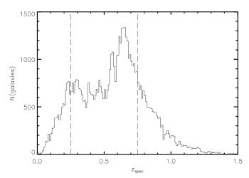
Figure 1.— $z_{spec}$ distribution of 62785 WiggleZ galaxies with redshift quality flag $Q_{zspec}$=3,4,5 at $z<1.5$ from four RCS2 patches. The redshift binsize is $\Delta z$=0.01. The WiggleZ selection function is designed to optimize observations of high-redshift galaxies thus a significant number of galaxies with $z\sim$0.3–0.6 are removed from the sample. In this paper we focus on the redshift range between $z$=0.25 and $z$=0.75, which are marked by the vertical dashed lines.

We focus on the redshift range between 0.25 and 0.75, giving a total of 41041 spectra. The lower $z=0.25$ boundary is chosen so that our bluest passband $g^{\prime}$ is still blueward of the 4000Å break at the lowest redshift bin, while the upper redshift limit is set based on having sufficient depth in the imaging data for the analysis of the companion galaxies.

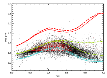
Figure 2.— The observed $g^{\prime}$-$r^{\prime}$ colors as a function of redshift for WiggleZ galaxies. Only 1/5 of the sample is plotted for clarity. The red, green, and blue solid curves are the colors from GISSEL evolving spetra described in §2.3, while the corresponding (dot-) dashed curves are the colors for the non-evolving spectra used for k-correction. A ‘hollow’ feature with a deficit of galaxies is observed at $z$=$\sim$0.3–0.6 and $g^{\prime}$-$r^{\prime}\sim$0.7 due to the ‘low-z rejection’ in the survey selection criteria. The red dots are galaxies that satisfy the ‘low-z rejection’ criteria but were still observed during early stages of the WiggleZ survey (before these criteria were fully implemented).

The observed $g^{\prime}$-$r^{\prime}$ colors of the WiggleZ galaxies as a function of redshift are presented in Figure 2. We also overplot three dust-free models generated from GISSEL (Bruzual & Charlot, 2003). The red dashed curve is the Single Stellar Population (SSP) model using the Padova (Bertelli et al., 1994) evolutionary tracks with solar metallicity $Z$=0.02 and the Chabrier (2003) IMF with a zero-redshift age of 13 Gyrs, representing evolved early-type red galaxies. The green dot-dashed curve is a $\tau$ model with an exponentially decreasing star-formation rate with $\tau=1$ Gyr, generated with a metallicity of $Z$=0.0001 and a zero-redshift age of 11 Gyr, representing mildly star-forming spiral galaxies. The cyan short-dashed line is a model made with a constant star formation rate, representing star-forming late-type/irregular galaxies.

We observe two features from Figure 2. First, red elliptical galaxies are absent from the WiggleZ sample. Most of the galaxies populate the region between the $\tau$- and constant star-formation models. This is expected, because the WiggleZ galaxies are selected by the UV flux to be star-forming galaxies.

Second, there is a ‘hollow’ region with a deficit of galaxies at $g^{\prime}$-$r^{\prime}$$\sim$0.7 between $z\sim 0.3-0.6$. This is also manifested as a dip in the redshift distribution of the WiggleZ markers at $0.3<z<0.6$ in Fig. 1. This ‘hollow’ feature arises artificially due to the ‘low-redshift rejection’ (LRR) criteria based on $g^{\prime}-r^{\prime}>0.6$ and $r^{\prime}-z^{\prime}<0.7(g^{\prime}-r^{\prime})$ in the WiggleZ’s selection criteria used in the RCS2 regions, in the attempt to maximize $z\geq 0.5$ galaxies. Thus, the LRR criteria actually remove galaxies at redshift up to $z\sim 0.6$, producing the significant broad dip in the redshift distribution of the WiggleZ galaxies. Nevertheless, the ‘hollow’ region has more galaxies in it than expected with the LRR criteria. There are 8597 galaxies in the sample that actually meet the LRR criteria but are still included in the WiggleZ sample. This is because the LRR criteria were developed after the early observing runs and thus some galaxies which were initially observed would have been rejected later on by the refined selection criteria. We find that these galaxies, overplotted in Fig. 2 as red dots, are primarily distributed over $0.25\leq z\leq 0.65$. Thus, while the WiggleZ survey intends to target blue star-forming galaxies, an examination of Figure 2 indicates that the sample is composed of a range of star-forming galaxies, with colors consistent with starburst to constant and mildly star-forming galaxies.

Finally, we note that any direct comparison of the properties in this spectroscopic sample as a function of redshift is not straightforward, due to the $20\leq r^{\prime}\leq 22.5$ selection criterion. This criterion produces galaxy samples of different absolute magnitude ranges at different redshifts.

2.4. The RCS2 Cluster WiggleZ Spare-Fibre (RCS-WSF) Sample

During the WiggleZ observing runs, a small number of AAOmega fibres were used for targets from different projects, using identical observation parameters and data reduction techniques. In addition to the sample of the UV-selected WiggleZ galaxies, there are $\sim$3000 spectra targeting RCS2 cluster galaxies as part of the WiggleZ-RCS2 collaboration. These galaxies are selected from a preliminary sample of RCS2 clusters at $z\leq 0.5$, chosen as possible high ranking, bright, red-sequence galaxies in the clusters. Most of these galaxies are at $z<0.45$ and have a mean redshift of $z\sim$0.28. The details and scientific results using this WiggleZ-RCS2 cluster subsample will be presented in a future paper. For the purpose of this work, they serve as an excellent comparison sample of markers to the WiggleZ galaxies, as they are red galaxies in dense environments. Since these galaxies do not cover the same redshift range as the WiggleZ galaxies, the comparison is only available at lower redshifts. We will refer to this sample as the RCS2 WiggleZ Spare-Fibre, or RCS-WSF, sample for the remainder of the paper.

3. Method

With the assumption that the WiggleZ marker galaxies and their neighbors reside in the same spatial regions, we can construct a net color-color-magnitude (CCM) cube of the neighbor galaxies, so the colors and magnitude information of the neighbor galaxies can be preserved. The $xyz$ axes of the cube represent $r^{\prime}-z^{\prime}$, $g^{\prime}-r^{\prime}$, and $r^{\prime}$, respectively. Thus, the net counts as a function of luminosity in the $r^{\prime}$ passband, for instance, can be computed by summing the values in the $x$ and $y$ axes along the $z$ axis. Essentially, we adopt the method used in Gilbank et al. (2008) and Loh et al. (2008) for creating color-magnitude diagrams, but extend the concept to a 3D cube. To produce the net CCM cube, we subtract a background CCM cube from the total-count CCM cube. The cubes are made in both observed and rest frames. We detail the methods below.

3.1. Observed Color-Color-Magnitude Cubes

To construct a CCM cube, we first identify all galaxies in the RCS2 photometric catalogs with $r^{\prime}\leq 24.0$ within a projected comoving radius of $r_{p}$ Mpc to a WiggleZ galaxy. The WiggleZ galaxy itself is excluded in this process. These galaxies are namely the ‘neighbors’ to the WiggleZ galaxy, and their observed $r^{\prime}-z^{\prime}$, $g^{\prime}-r^{\prime}$, and $r^{\prime}$ are gridded into a cube with a binsize of 0.05, 0.05, and 0.1 along the $xyz$ (color-color-magnitude) axes. The CCM cube of the control field (i.e., the background) is constructed using all galaxies with $r^{\prime}\leq 24$ in the same RCS2 patch. A single RCS2 patch is sufficiently large (typically 81 square degrees) to provide excellent background statistics, and by using the same patch, it also ensures a minimal systematic effect. The control cube has the same binsize as the cube of the marker neighbors. The count of each element in this control cube is then scaled by $N_{ran,in}/N_{ran,tot}$, which is the ratio of the number of the random points within the aperture ($N_{ran,in}$) to the total count ($N_{ran,tot}$) in the patch (see §2.2). The typical $N_{ran,in}/N_{ran,tot}$ is $\sim$ $2\times 10^{-6}$. A net CCM cube is obtained by subtracting the scaled control cube from the cube of the neighbor galaxies, i.e.,

$$\rm cube_{net}=cube_{neighbor}-cube_{background}\times~{}N_{ran,in}/N_{ran,tot}.$$

These net CCM cubes from individual markers can then be stacked to form the total CCM cube.

3.2. Rest-Frame Color-Color-Magnitude Cubes

One approach to obtain a rest-frame CCM cube is to convert it from an observed one which has been described above. However, it requires a large amount of computing time to k-correct each element of an observed CCM cube. An alternative is to compute the rest-frame magnitude and colors of each galaxy first, then construct the rest-frame CCM cube using the same procedure as building the observed cube. Since there is no actual redshift information for the neighbors, it is assumed that all surrounding galaxies are at the same redshift as the marker. A control field cube is computed for each marker, for which we also convert all galaxies into “rest-frame photometry” using the redshift of the WiggleZ galaxy.

The k-correction is derived using tables generated for each of the GISSEL (Bruzual & Charlot, 2003) models described in §2.3. Each table contains galaxy colors of the model and the k-correction values for each passband as a function of redshift. For a galaxy at a fixed redshift, we derive the k-correction using the model grid by interpolating (or extrapolating in some instances) the model colors to match the observed galaxy colors. The model colors here are the observer-frame colors of GISSEL galaxies with non-evolving spectra, which are overplotted as curves in Figure 2. We use the $g^{\prime}-r^{\prime}$ color to derive k-corrections for the $g^{\prime}$ and $r^{\prime}$ passbands, and $r^{\prime}-z^{\prime}$ for the $z^{\prime}$ magnitude. We have compared our k-correction results to the SDSS galaxies in one region, where their k-corrections are available from the official SDSS database. Our method in deriving the k-correction yields a good correlation with the SDSS values. We use $z=0.5$ as our reference redshift, and all the rest-frame photometry is computed relative to this redshift as ${}^{0.5}M=m-DM-(k-k_{z=0.50})$, where $DM$ is the distance modulus. For reference, Figure 3 plots the k-correction as a function of redshift for each filter for the three spectral types.

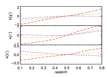
Figure 3.— k-correction as a function of redshift for $g^{\prime}r^{\prime}z^{\prime}$ filters. The dashed red, dot-dashed green, and short-dashed purple curves are generated using the same model in Fig. 2, which represent evolved early-type red, mildly star-forming spiral, and star-forming late-type/irregular galaxies respectively.

4. Results

In this section we derive the various photometric properties of the galaxy population associated with the WiggleZ marker galaxies. Our sample is limited to $0.25\leq z<0.75$, and is divided into five redshift bins with $\Delta z$=0.10. We refer to these redshift bins as $z=$ 0.3, 0.4, 0.5, 0.6 and 0.7. We group the WiggleZ galaxies into the redshift bins, and stack all the net CCM cubes within each redshift bin. The numbers of the markers and their neighbors in each redshift bin are listed in Table 1. A total of 45,198 net galaxy counts around 41,041 markers are used in our analysis. All the CCM cubes are made using galaxies within a projected comoving radius $r_{p}$=0.25Mpc from the markers. The choice of this $r_{p}$ will be justified in §4.2. The CCM cubes of the RCS-WSF sample presented in §4.5 are made with an angular-diameter radius of $r_{p}$=0.25Mpc instead of a comoving one, since cluster galaxies are considered gravitationally bound, although the results are similar when using either a comoving or angular-diameter radius due to their redshift range. The galaxy counts in the RCS-WSF sample are tabulated in Table 2. The average number of net companions to the markers in this sample are about an order of magnitude larger than that for the WiggleZ sample.

Table 1Galaxy Counts

redshift	$N_{WiggleZ}$	$N_{net}$	$N_{background}$
0.25–0.35	6885	10332.0	118828.0
0.35–0.45	6090	7811.85	61085.1
0.45–0.55	6857	8021.05	46571.0
0.55–0.65	10869	9948.05	54039.0
0.65–0.75	10340	9084.79	40491.2

Table 2Galaxy Counts for the RCS-WSF Sample

redshift	$N_{RCS-WSF}$	$N_{net}$	$N_{background}$
0.25–0.35	416	8968.30	12270.7
0.35–0.45	294	4760.45	5754.54

4.1. Random Marker Fields

To test the reliability of background subtraction in our method, we construct CCM cubes based on the positions of 4000 randomly drawn points from the random catalogs in each of the four RCS2 patch. These random points are then assigned a redshift between $z$=0.25 and $z$=0.75. This gives us $\sim$3200 random points in total for each redshift bin. All the CCM cubes are built in the same way as described in §3 but with the marker position and redshift replaced. Because these markers are randomly chosen and not based on actual positions of any galaxy, we expect the average net excess in the neighbor counts to be zero when these net CCM cubes are stacked, if the background subtraction is properly handled.

We compute a net neighbor count, $N_{net}$, for each random point by summing the intensity in all elements of an observed-frame net CCM cube built with $r_{p}$=0.25Mpc. The $N_{net}$ distribution together with its dependence on galaxy magnitudes and colors are plotted in Fig. 4.

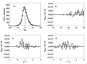
Figure 4.— The $N_{net}$ of the random catalogs computed using $r_{p}$=0.25Mpc. a): distributions of the $N_{net}$ for the 4000 random markers in each RCS2 patch. b), c), d): The mean $N_{net}$ per bin ($\Delta r^{\prime}=0.1$, $\Delta(g^{\prime}-r^{\prime})=0.05$, or $\Delta(r^{\prime}-z^{\prime})=0.05$) along each axis of the stacked cube over $0.25\leq z<0.75$. No systematic offset is observed.

Panel a) shows the $N_{net}$ distributions of the 4000 random markers in each RCS2 patch. These distributions are statistically identical for the different patches. Summing these distributions gives a median $N_{net}=-0.344$ and a mean $N_{net}=0.032\pm 0.027$ galaxies, where the uncertainty is the rms of the mean. Thus, the mean of the net counts around random points is consistent with being zero. The relatively large negative value of the median of the net counts is the result of galaxies being clustered even on the projected sky, which results in a skewed histogram of the net count distribution. Because there is no observed offset in $<N_{net}>$ among different redshift bins, we stack all the cubes over $0.25\leq z<0.75$, and project the stacked cube along an axis of $r^{\prime}$, $g^{\prime}-r^{\prime}$, or $r^{\prime}-z^{\prime}$. The total $N_{net}$ of the stacked cube along each axis is presented in the b), c), and d) panels in the Figure. The $<N_{net}>$ counts are also not a function of magnitude and colors, and have means of essentially 0, indicating that the background contamination is correctly subtracted, statistically speaking. Given these results, we are confident of our method in background correction and constructing the CCM cubes.

4.2. Net Excess Galaxy Surface Density

The WiggleZ survey targets blue star-forming galaxies with a set of complex selection functions. Blue star-forming galaxies are believed to populate less dense environment compared to red passive galaxies (e.g., Dressler et al., 1980; Weinmann et al., 2006; Cooper et al., 2007). To investigate the characteristics of the neighborhood of WiggleZ galaxies, we probe the total net neighbor counts, $N_{net}$, as a function of radius centered at each WiggleZ galaxy. The observed CCM cubes in a series of annuli are computed, and $N_{net}$ in an annulus is the sum of the intensity of all elements in the cube. Even though all the observed CCM cubes are constructed using galaxies to a fixed apparent magnitude of $r^{\prime}$=24.0, we note that the comparison among different annuli at a fixed redshift bin is still meaningful. Direct comparisons among different redshift bins, however, cannot be made because the cubes are not limited to the same absolute magnitude depth for the different redshift bins.

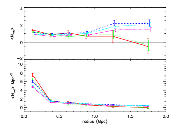
Figure 5.— The differential mean $N_{net}$ in each annulus without (top) and with (bottom) area normalization. In each panel, the solid red, dotted green, dashed blue, dot-dashed cyan, and dot-dot-dashed pink curves represent our redshift bins in an increasing order. There are $\sim$1.5 net excess galaxies within $r_{p}$=0.25Mpc, giving a surface density of $\sim$6 gal/Mpc². The surface density drops quickly to $\sim$0 gal/Mpc² at $r_{p}\geq 1.5$Mpc.

The mean $N_{net}$ in each annulus for the different redshift bins are plotted in Fig. 5 as a function of $r_{p}$. The number of net excess galaxies within an annulus is not large, the maximum being only $\sim$1.5 within $r_{p}$=0.25 Mpc. Normalizing the $N_{net}$ by the aperture size, the mean surface density is a strong function of radius, being $\sim$6 gal/Mpc² within $r_{p}$= 0.25Mpc and then decreasing rapidly with increasing radius and reaching $\sim$0 at $r_{p}\geq 1.5$ Mpc. Because most $N_{net}$ excess is observed within 0.25 Mpc, we therefore use $r_{p}$=0.25 Mpc to construct the observed- and rest-frame CCM cubes for our further analysis.

4.3. The WiggleZ Galaxies and their Neighbors

4.3.1 Observed Color-Color Diagrams

Observationally speaking, galaxies appear to be primarily divided into two classes. One is red passive galaxies and the other, blue star-forming galaxies. These two classes of galaxies form the so-called ‘red sequence’ and ‘blue cloud’ in color-magnitude space. In fact, red galaxies may be a mix of truly old passive galaxies and dusty star-forming galaxies, and they cannot be distinguished well using a single optical color. However, Wolf et al. (2005) showed that dusty star-forming galaxies can be well separated from old passive ones in a color-color space, as long as one color brackets the 4000Å break and the other is at a longer wavelength. They found that dusty red galaxies actually form a continuous tail extending from the blue cloud, while old red galaxies form a separate structure of their own (the red sequence). This makes the color-color diagram a powerful diagnostic tool.

Figure 6 presents the observed color-color diagrams for neighbors in 5 redshift bins, where the colors of the three models from Figure 2 are overlaid as crosses for reference. For better visual presentation, the pixels ($\Delta(g^{\prime}-r^{\prime})\times\Delta(r^{\prime}-z^{\prime})$) in the color-color intensity plot are subdivided by a factor of 4 into smaller pixels in units of 0.0125 mag, and then smoothed by a kernel of 10$\times$10 pixels. The intensity scale is in units of counts per small pixels after normalizing the net counts to $1\times 10^{4}$ in each redshift bin. We also overplot the WiggleZ galaxies as the non-filled contours with a $\Delta$($r^{\prime}$-$z^{\prime}$)=1 offset for clarity.

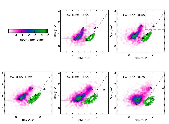
Figure 6.— Observed color-color diagrams at five redshift bins. The total net count is normalized to 1$\times 10^{4}$ in each panel. The intensity plot is in counts per pixel of 0.0125$\times$0.0125 mag. The WiggleZ galaxies are plotted as the non-filled contours with a level of 10 galaxies, but shifted by $\Delta$($r^{\prime}$-$z^{\prime}$)=1 for clarity. The WiggleZ LRR criteria are shown as the black dotted lines, with the $r^{\prime}-z^{\prime}$ shifted as well. The crosses are the colors of three model galaxies with evolving spectra shown in Fig. 2, and their colors shifted by $\Delta$($r^{\prime}$-$z^{\prime}$)=1 are plotted as the triangles. Both the WiggleZ galaxies and the neighbors form a continuous sequence at each redshift, with the majority of them populated in a blue region. The contamination of dusty star-forming galaxies, indicated by the dashed box, is insignificant for both the markers and the neighbors.

We observe that, for all redshift bins, both the WiggleZ galaxies and most of their neighbors populate a similar color-color plot, with the exception that the WiggleZ galaxies do not show a clump of red-passive galaxies. They both exhibit a continuous sequence in all redshift divisions. The sequence runs from the blue star-forming regions toward the red passive area, marked by the model colors; but no WiggleZ markers have colors as red as the red passive galaxies, indicating that they contain little dust. We note that this is likely a reflection of the survey design, as the WiggleZ galaxies are selected primarily by UV fluxes.

Although most of the neighbor galaxies reside in the star-forming sequence, some neighbors populate the region of passive red galaxies. These red neighbors are red-sequence galaxies, and we will discuss their properties later in the paper. Some neighbors in the lower-redshift bins, however, exhibit redder ($z^{\prime}-r^{\prime}$) colors than that expected from passive red galaxies at their fixed redshift, and form roughly a continuous sequence from the blue star-forming galaxies. These neighbors are possible dusty galaxies. We note that such estimation is approximate, since the regions in the color-color diagram for dusty reddened star-forming galaxies may change at different redshifts due to the shifting of the 4000Å break in observed frame. At $z\sim 0.6$ and beyond, the use of the current color-color diagram to distinguish between dusty star-forming and red passive galaxies is not optimal, because the 4000Å break is shifted beyond the center of the $r^{\prime}$ passband, and having only one passband ($z^{\prime}$) at longer wavelengths is not sufficient to distinguish between passive and dusty SEDs. Using a rough color cutoffs to define dusty galaxies as $(r^{\prime}-z^{\prime})-C_{E}>0.3$ and $g^{\prime}-r^{\prime}\geq\Delta C$ where $C_{E}$ is the color of the red elliptical model in Figure 2 and $\Delta C$ is the color halfway between the red and green models in the same Figure, we estimate about 5.2$\pm$1.0%, 2.4$\pm$0.8%, and 0.2$\pm$0.5% of the galaxies in the three lower-redshift bins in increasing redshift order may be dusty star-forming galaxies. From these fractions, we conclude that dust reddened star-forming galaxies are not likely a significant component in the WiggleZ neighbors, at least for $z\lower 0.43057pt\hbox{\hbox to0.0pt{\raise 2.58334pt\hbox{\hskip 1.29167pt{{$\scriptscriptstyle<$}}}\hss} \kern-1.72218pt{{$\scriptscriptstyle\sim$}}}0.6$. Note that the decrease in the dusty galaxy fraction is likely due to the shifting of the $r^{\prime}$ towards the 4000Å break and possibly the different luminosity depths in the redshift bins, and does not necessarily reflect a real change.

4.3.2 Control for the Star-Formation Rate of the Markers

Since the star-formation properties of the WiggleZ galaxies themselves are not uniform across redshift due to the complex selection criteria, we want to examine whether the properties of the neighbors vary with the star-formation activity of the WiggleZ markers. We use the [OII]$\lambda$3727Å emission line equivalent width (EW) of the WiggleZ markers as the proxy for the specific star-formation rate of the markers and probe where neighbors around markers with different EW([OII]$\lambda$3727Å) populate the observed color-color diagrams.

First, we measure the [OII]$\lambda$3727Å equivalent width of the markers. The observed spectra have weak continuum due to the short exposure time ($\sim$1hr), hence the measured EW is noisy for the fainter galaxies. To measure the EW([OII]$\lambda$3727Å), we define a window of 10Å centered at 3727.8Å as the region for the [OII]$\lambda$3727Åline. The continuum level is determined using a window of 30Å on each side of the [OII] line (on the rest frame), starting at 3677.8Å and 3757.8Å. Either a linear or second-order polynomial function, whichever returns the smallest $\chi^{2}$, is chosen to describe the fitted continuum within the windows. The spectrum is then subtracted by this fitted continuum. A bi-Gaussian function is then applied based on the data points within all three windows. The flux of the [OII]$\lambda$3727Å line is accordingly the total net flux under this fitted bi-Gaussian curve. We divide the WiggleZ galaxies into three bins based on the 33.3% percentiles of the EW([OII]$\lambda$3727Å) at each redshift bin. Galaxies without any [OII]$\lambda$3727Å detection are excluded. The median and the 1$\sigma$ uncertainty of the computed EW([OII]$\lambda$3727Å) are about 112.5$\pm$32.6Å and 17.7$\pm$8.0Å for the highest and lowest EW([OII]$\lambda$3727Å) bins at $z$=0.25-0.35, respectively.

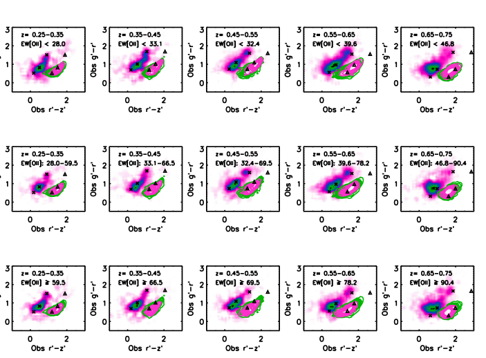
Figure 7.— Observed color-color diagrams for the WiggleZ and their neighbors where the markers are controlled for their EW([OII]$\lambda$3727Å). The total intensity for the neighbors in each panel is normalized to a total count of 1$\times 10^{4}$, and on the same scale as Fig. 6. The WiggleZ galaxies are plotted as the open pink contours with a level of 10 galaxies. The green contours are those in Fig. 6 for all the WiggleZ markers at a fixed redshift bin as reference. Within the same redshift bin, both the $g^{\prime}-r^{\prime}$ and $r^{\prime}-i^{\prime}$ color distributions of the WiggleZ galaxies and their neighbors remain similar for samples with different EW([OII]$\lambda$3727Å), indicating that the specific star-formation rate of the parent markers does not affect the properties of the neighbors.

We re-stack the observed CCM cubes of the neighbors by dividing the sample into bins of EW([OII]$\lambda$3727Å) within each redshift bin and present them in Figure 7, where the WiggleZ markers themselves are again offset by $\Delta(r^{\prime}-z^{\prime})=1$ for clarity. From Figure 7, it is clear that the color-color distributions for neighbors of WiggleZ galaxies of different EW([OII]) are very similar within the same redshift bin. Kolmogorov-Smirnov tests of pairs of both $g^{\prime}-r^{\prime}$ and $r^{\prime}-z^{\prime}$ distributions find no significant difference between the different EW([OII]$\lambda$3727Å) bins within the same redshift bin. The smallest significant level in all the pair-wise comparisons is 0.22. This implies that the properties of the neighbors do not strongly depend on the properties of the WiggleZ galaxies. Furthermore, we find that the $N_{net}$ distributions of the neighbors within 0.25 Mpc, although not shown here, are identical among all WiggleZ galaxies with different EW([OII]$\lambda$3727Å) at a fixed redshift bin. This adds to the growing evidence that environment has little influence in the properties of star-forming galaxies (e.g., Balogh et al., 2004; Yee et al., 2005; Carter et al., 2001; Rines et al., 2005; Cassata et al., 2007; Balogh et al., 2009). Therefore, we conclude that the insignificant dependence between the properties of the neighbors and the markers allows us to explore galaxy evolution using the neighbors, even though the WiggleZ galaxies may cover different ranges of properties at different redshifts due to the survey selection criteria; for example, the $r^{\prime}$=20-22.5 criterion naturally select more massive galaxies at higher redshifts.

Since one of the primary WiggleZ target selection criteria is based on UV flux, we also check whether the $NUV$ luminosity of the markers affects the color properties of the neighbors. This is essentially testing whether the total star-formation rate of the markers affects the color-color distributions of the neighboring galaxies. To do so, we divide the markers into three groups in each redshift bin based on their rest-frame $NUV$ luminosity. Because the sample of the markers is not complete to the same rest-frame $NUV$ depth, direct comparisons between different redshift bins cannot be done. However, within the same redshift bin, we can compare the color-color distributions of the markers and their neighbors over its range of rest-frame $NUV$ luminosity. The result is presented in Fig. 8. As in the case for EW([OII]$\lambda$3727Å), we observe, and confirm with Kolmogorov-Smirnov tests, that within a fixed redshift bin the color distributions of the neighbors around markers with different $NUV$ luminosities are statistically identical. This supports our conclusion of Fig. 7 that the properties of the neighbors are not significantly affected by, or strongly correlated with, the characteristics of the markers. We also find that the optical color distributions of the markers themselves do not strongly depend on the absolute $NUV$ luminosity.

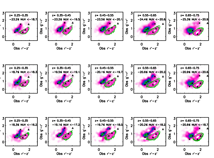
Figure 8.— Similar to Fig. 7 but controlling for the markers’ NUV luminosity. At a fixed redshift bin, both the colors of the neighbors and the markers themselves remain similar regardless of the NUV luminosity.

4.3.3 Control for AGN Candidates in the Markers

Since AGN activities in galaxies are sometime responsible for emission lines, we are also interested in whether the neighbors of the AGN hosts have similar properties as those of normal star-forming galaxies, i.e., the rest of the WiggleZ galaxies. The most common way to distinguish AGNs and star-forming galaxies is based on the ratios of [OIII]/$H_{\beta}$ and [NII]/$H_{\alpha}$ emission lines, the so-called BPT plot (Baldwin et al., 1981). This method works only at $z<0.48$ for the WiggleZ survey where all these emission lines can be detected within the spectral wavelength coverage. Recently Bongiorno et al. (2010) use a method similar to the BPT plot to separate AGNs and star-forming galaxies at $0.50\leq z\leq 0.92$, i.e., [OIII]$\lambda 5007$Å$/H_{\beta}$ versus [OII]/$H_{\beta}$, in the zCOSMOS survey. The separation in this diagnostic diagram was derived empirically using the observed data by studying the positions in the diagram of AGN and star-forming galaxies which were classified based on the BPT plot (e.g., Rola et al., 1997; Lamareille et al., 2004). We present the [OII]/$H_{\beta}$ vs [OIII]/$H_{\beta}$ plot for all our WiggleZ galaxies at $0.25\leq z\leq 0.75$ in Fig. 9,

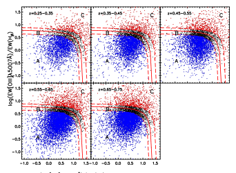
Figure 9.— Selection of AGN candidates. The WiggleZ galaxies are classified into three groups by the empirical separation used in Bongiorno et al. (2010). The galaxies in group A are primarily star-forming galaxies, while those in group C are possibly AGN hosts. Group B contains all the rest of the galaxies between group A and C, within the regions enclosed by two dashed red lines in the plot .

where we overplot the analytical expression of Eq. 3 of Bongiorno et al. (2010) for the demarcation curves between star-forming galaxies and AGNs. We divide the WiggleZ markers into three groups based on their locations on the [OII]/$H_{\beta}$ plot. Group A is those located below the analytical expression in the star-forming region. Group B contains a mix of star-forming and AGN galaxies, located in a narrow strip region centered at the analytical expression. Group C is the AGN candidates lying above the analytical expression. These groups contribute about 67%, 20%, and 13% of the galaxies, respectively.

We find that the neighbors of each group have similar $N_{net}$ distribution (Fig. 10), and occupy essentially identical regions on the color-color diagram. The $N_{net}$ here is computed using a limit of $M_{r^{\prime}}^{*}+1$ , with $M_{r^{\prime}}^{*}$ derived in §4.5. This echoes our conclusion that the properties of the neighbors are not strongly affected by the properties of the markers themselves. Our results suggest that WiggleZ galaxies hosting AGN are in environments similar to other WiggleZ galaxies. This conclusion is consistent with other more detailed studies of Seyfert galaxies that the average environment of their hosts is not significantly different from other galaxies of similar properties (e.g., De Robertis et al., 1998; Schmitt, 2001).

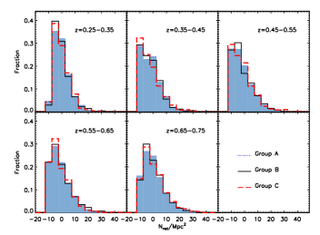
Figure 10.— The $N_{net}/Mpc^{2}$ distributions of each group in Fig. 9, presented as filled blue, thin black, and thick red histograms, respectively. The $N_{net}$ is computed using the $M_{r^{\prime}}^{*}+1$ limit. Each histogram has a binsize of 5. All these these groups have similar $N_{net}/Mpc^{2}$ distributions at each redshift.

4.4. Rest-Frame Color-Magnitude Diagrams

Figure 11 presents the rest-frame color-magnitude diagrams for the WiggleZ neighbors in redshift bins of $z\sim$0.3 to $z\sim$0.7. These are made by summing the elements of the color-color-magnitude cubes along the $x$-axis (i.e., $r^{\prime}$-$z^{\prime}$ axis).

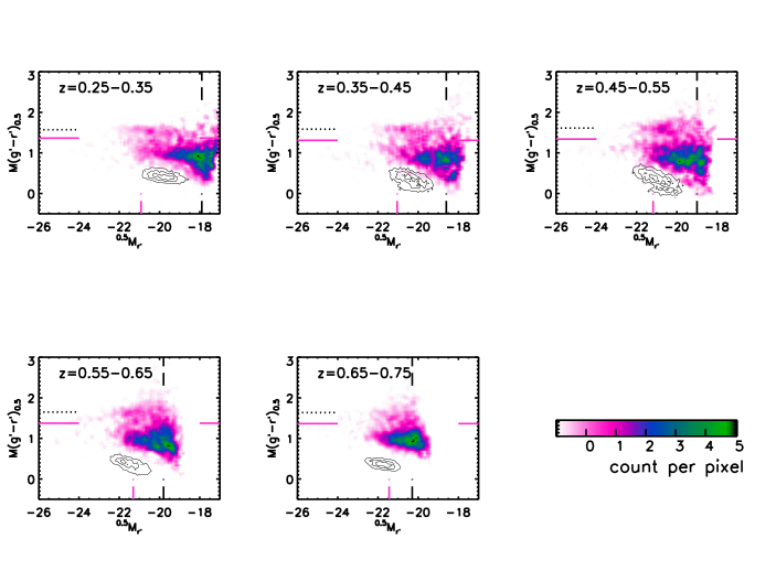
Figure 11.— The rest-frame color-magnitude of the WiggleZ neighbors at each redshift. The intensity of each panel is normalized to a total count of 1$\times 10^{4}$, and is in units of counts per pixel with a size of 0.0125$\times$0.025 (color$\times$magnitude) mag. The vertical pink dashed lines mark the derived ${}^{0.5}M_{r^{\prime}}^{*}$ for the ‘All’ subsample in §4.5. The horizontal solid line in each panel marks the separation between blue and red galaxies. The color of the red sequence is indicated by the horizontal dotted line. The black vertical dashed lines mark the ${}^{0.5}M_{r^{\prime}}$ limit. The red sequence of the neighbor galaxies is observable at each redshift. For reference, the WiggleZ galaxies themselves are overplotted as the green contours shifted by –0.5 magnitudes in $M(g^{\prime}-r^{\prime})_{0.5}$.

Based on the conclusion in the previous two subsections (§4.3.2 and §4.3.3) that the properties of the neighbors are not strongly dependent on the properties of the WiggleZ galaxies themselves, the comparisons of the color-magnitude diagrams at difference redshifts can provide us useful insights into galaxy evolution.

The first observation we can glean from the Figure is that the WiggleZ neighbors populate regions of both the red sequence and the blue cloud at each redshift bin. The majority of them are in the blue cloud. A gap between the red sequence and blue cloud is seen. In general, the red sequence at each redshift can be approximated by a horizontal line of the color of early-type galaxies. The flatness of the red-sequence is more likely a result of the relatively low signal of the red-sequence galaxies in our data, making them insufficient for deriving an accurate fit, rather than due to the nature of the red sequence. The dispersion in the red sequence appears to be larger at higher redshift; however, this can be mostly attributed to the larger photometric uncertainties for galaxies in these subsamples. We also plot on Figure 11 the color-magnitude distribution of the WiggleZ galaxies in each redshift bin as contours, shifted by –0.5 mag in $g^{\prime}-r^{\prime}$ color. We note that the WiggleZ galaxies are primarily distributed along the bright blue edge of blue-cloud galaxies, reflecting that they are strong star-forming galaxies.

4.5. Galaxy Luminosity Function

The galaxy luminosity function (GLF) offers a convenient tool in exploring the different components of the galaxy population in a sample. The most widely used form for the GLF is the Schechter function (Schechter, 1976), which can be characterized by three parameters: the normalization density $\phi^{*}$, the characteristic magnitude $M^{*}$, and the faint-end slope $\alpha$. It has been found that $\alpha$ depends strongly on the galaxy SED type. The redshift evolution of the GLF, however, is also strongly dependent on SED types (e.g., Wolf et al., 2003; Liu et al., 2008; Salimbeni et al., 2008). The GLF for early-type galaxies are described better with a shallower (sometime, down-turning) $\alpha$, and they are more abundant towards low redshift. In contrast, late-type galaxies have a GLF with a steep $\alpha$, and their number density is largely unchanged toward low redshift. In this subsection, we explore the GLF for the WiggleZ neighbors, and investigate the galaxy population components by examining the shape of their GLF and their evolution.

4.5.1 Constructing the GLF

The GLF of the neighbors is constructed by projecting the CCM cube along the $z$-axis (i.e., the $r^{\prime}$ magnitude) to produce counts as a function of $r^{\prime}$ magnitude. We have conducted and cross-checked the analyses using both the observed and rest-frame CCM cubes. Here, we present only the results using the rest-frame CCM cubes, for which $g^{\prime}$, $r^{\prime}$, and $z^{\prime}$ have been k-corrected to $z$=0.50. We note that the observed $r^{\prime}$-band at $z=0.5$ is approximately equivalent to the rest $B$ band.

We also separate the neighbors into red and blue populations. The division between the red and blue populations is chosen to be the $g^{\prime}-r^{\prime}$ color half way between the non-evolving early-type and the star-forming $\tau$ model of Figure 2 at each redshift, equivalent to 0.27 mag bluer than the red-sequence color. To adjust for minor systematic effects in the photometry, the $g^{\prime}-r^{\prime}$ color (at rest $z=0.5$) of the red-sequence in each redshift bin in Fig. 11 is determined empirically as the reference. This is done by examining the $g^{\prime}-r^{\prime}$ color distribution of galaxies in each redshift bin which are brighter than ${}^{0.5}M_{r^{\prime}}^{*}+1$ and have colors redder than $(g^{\prime}-r^{\prime})_{rs}-0.27$, where $(g^{\prime}-r^{\prime})_{rs}$ is the non-evolving rest-frame model early-type galaxy color of Figure 2. The distribution is fitted with a Gaussian, and the peak is used as the red-sequence color. The red-sequence colors and the boundaries between the red and blue populations are indicated in Fig. 11 by the dotted and solid horizontal lines, respectively. We note that the computed $g^{\prime}-r^{\prime}$ red-sequence colors are essentially identical to those of the models, with the exception of the $z=0.3$ bin, where the $g^{\prime}-r^{\prime}$ separation for red and blue galaxies appears to be $\sim$0.06 bluer than the computed color of $(g^{\prime}-r^{\prime})_{rs}-0.27$.

The GLF results are presented in Figure 12. We denote the three subsamples of galaxies and their GLF as ‘All’, ‘Blue’, and ‘Red’. The errors in the y-axis in each $r^{\prime}$ bin is computed using Poisson statistics. We also compute the GLF using the same method for the RCS-WSF sample for comparison with the WiggleZ neighbor galaxies at the two lower redshift bins, allowing us to examine the effects of environment on galaxy evolution. The CMD and the resultant GLFs for the cluster sample are plotted in Fig. 13.

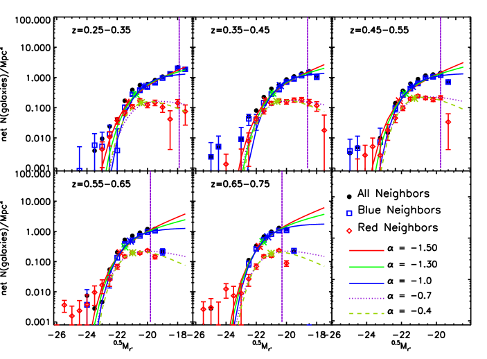
Figure 12.— The $r^{\prime}$-band luminosity function for all the neighbors of the WiggleZ galaxies. The red, green, and blue curves are the fitted Schechter LF with $\alpha$=-1.50, 1.30, and -1.0, respectively. The Schechter LF for the red neighbors are described by $\alpha$= -0.70 and -0.40 shown as the dotted purple and dashed green curves. The vertical purple line marks the sample complete limit. The GLF for the ‘All’ and ‘Blue’ neighbors are better described by a steeper $\alpha$ than that to the ‘Red’ subsample.

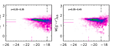
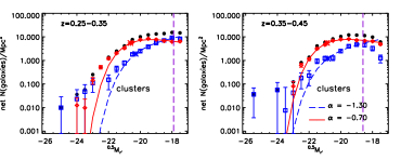
Figure 13.— The color-magnitude diagrams (Top) and luminosity functions (Bottom) for the RCS-WSF sample for the lowest two redshift bins. The red-sequence galaxies are dominant in both the plots. The symbols are of the same meaning as Fig. 12.

4.5.2 The Schechter Function Fit

We fit the GLF discussed above using the Schechter function. We determine the completeness limit in ${}^{0.5}M_{r^{\prime}}$ for each redshift bin by examining the total net counts in 0.1 magnitude bins as a function of ${}^{0.5}M_{r^{\prime}}$, smoothed by a three-bin kernel. We use the bin 0.1 mag brighter than the peak as the limit for fitting the Schechter function, giving ${}^{0.5}M_{lim}=$ [–17.9, –18.6, –19.0, –19.8, –20.3] for the five redshift bins. These limits are marked as vertical purple (dashed) lines in Fig. 12.

To investigate the shape of the GLF, we first allow $\alpha$ to vary in fitting the Schechter function. The results of the Schechter function fits are tabulated in Table 3. As evident from the CMD (Fig. 11), the GLFs in Fig. 12 of the WiggleZ neighbor galaxy populations are dominated by blue galaxies. It is not surprising that the GLFs of the ‘All’ and the ‘Blue’ subsamples are similar, because $\sim 80$% of the neighbors are blue galaxies.

For the ‘Blue’ and ’All’ samples, we find that the fitted $\alpha$ appear to become less steep at higher redshift. However, this could in part be the result of the different sampling magnitudes in the subsamples; the shallower absolute magnitude limits in the higher redshift bins make $\alpha$ less well-determined. This is especially true at the highest redshift bin, where the completeness limit is only about 1 to 1.5 mag past $M^{*}$. Discarding the $z=0.7$ bin, the derived $\alpha$ for the ‘All’ and ‘Blue’ subsamples range between $\sim-1.0$ and $\sim-1.5$, comparable to those in the literature for star-forming or late-type galaxies (e.g., Wolf et al., 2003; Christlein et al., 2009; Liu et al., 2008). The possibility that the apparent changes in $\alpha$ at different redshifts are due to the change in the sampling limit can be demonstrated by fitting the three low-redshift bins for the ‘Blue’ subsample to a common limit of ${}^{0.5}M_{r^{\prime}}=-19.0$, which is complete for the three bins. We obtain the results: $\alpha=$ [$-1.15\pm 0.17$, $-1.38\pm 0.16$, $-1.03\pm 0.12$] for $z=$ [0.3, 0.4, 0.5], which are consistent with being identical at $\sim 1.75\sigma$.

We overplot the Schechter LF in Fig. 12 with fixed $\alpha$=[-1.50, -1.30, -1.00] fitted for the ‘Blue’ subsamples to show the ability of the data to distinguish between the faint-end slopes within this range. By combining the three lower-redshift bins ($0.25<z<0.55$) where the data are of sufficient depth to obtain a robust measurement of $\alpha$, we find for the ‘Blue’ galaxies a best-fit $\alpha$ of $-1.18\pm 0.08$. For consistency of comparison of ${}^{0.5}M_{r^{\prime}}$ among redshift bins, we adopt an $\alpha$ of $-1.3$ for all redshift bins, and tabulate the fitted ${}^{0.5}M_{r^{\prime}}^{*}$ in Table 3.

The best fitting results for ${}^{0.5}M_{r^{\prime}}^{*}$ and $\alpha$ for the WiggleZ ‘Red’ neighbor galaxy samples at different redshift bins are also presented in Table 3. For the lower redshift bins, where the data are of sufficient depth, the GLF is considerably less steep at the faint-end compared to that of the ‘Blue’ subsample. At higher redshifts, the red GLFs can be described by a steeper $\alpha$, but this is again likely because the faint-end of the GLF is not observable at these redshifts. We use the three lower redshift bins to establish a more robust estimate of the faint-end slope of the red galaxy GLF. We obtain $\alpha=-0.45\pm 0.13$ by summing the data (to ${}^{0.5}M_{r^{\prime}}=-19.0$) in these bins.

For the purpose of comparison, we perform the same analysis for the RCS-WSF sample of markers in RCS2 clusters. Here, the CMD shows a very strong red sequence and the total GLF is dominated by red galaxies, as shown in Figure 13). The faint-ends of the ‘Blue’ galaxy GLF in the two redshift bins have a similar $\alpha$ as those for the corresponding subsamples of the WiggleZ neighbors. For the purpose of comparing $M^{*}$, we also fit the RCS-WSF ‘Blue’ samples using $\alpha$ = [-1.50, -1.30, -1.00] with the results listed in Table 4.

Opposite to the WiggleZ neighbor samples, the GLF of the RCS-WSF sample of cluster galaxy targets is dominated by the ‘Red’ galaxy sample. The faint-end slope for these red galaxies appears to be significantly steeper than that of the WiggleZ counterpart, with $\alpha$ steeper than –0.65. The combined ‘Red’ GLF for the two redshift bins of the RCS-WSF data produces a best fitting $\alpha=-0.74\pm 0.06$. A similar combination for the WiggleZ neighbor sample produces $\alpha=-0.18\pm 0.17$. In order to provide a consistent comparison for the ${}^{0.5}M_{r^{\prime}}^{*}$ values for the ‘Red’ WiggleZ neighbor sample and the ‘Red’ RCS2 cluster neighbor sample, we also refit all the red galaxy subsamples using $\alpha=-0.4$ and –0.7, and the results are tabulated in Table 3.

4.5.3 The Evolution of ${}^{0.5}M_{r^{\prime}}^{*}$

We examine the evolution of the $M^{*}_{r^{\prime}}$ parameter of the Schechter LF by assuming a simple linear dependence between $M^{*}_{r^{\prime}}$ and redshift, as used by Lin et al. (1999) and others. We can write: ${}^{0.5}M_{r^{\prime}}^{*}(z)$=$m_{r^{\prime}}^{*}-DM-(k-k_{z=0.50})+Q(z-0.5)$, where $DM$ is the distance modulus and $k$ is the k-correction. The evolution term $Q$ is derived from a linear fit to ${}^{0.5}M_{r^{\prime}}^{*}$ as a function of redshift in the form of ${}^{0.5}M_{r^{\prime}}^{*}(z)$ = ${}^{0.5}M_{r^{\prime}}^{*}(z=0.5)+Q(z-0.5)$. The derived $Q$ depends on the value of $\alpha$; a steeper $\alpha$ results in a smaller $Q$. Because the fitted $\alpha$ and $M_{r^{\prime}}^{*}$ correlate with each other and $\alpha$ are marginally different in our redshift divisions, we use the $M_{r^{\prime}}^{*}$ derived with $\alpha=-1.30$ for the ‘All’ and ‘Blue’ subsamples and $\alpha$= –0.40 for the ‘Red’ neighbors, obtaining $Q$=[$-1.31\pm 0.24$,$-2.10\pm 0.26$,$-1.59\pm 0.30$] for the ‘All’, ‘Blue’, and ‘Red’ subsamples, respectively. The results are shown in Fig. 14 and tabulated in Table 3. We also derive $Q$ using $\alpha=-1.0$ and –1.5 for the ‘All’ and ‘Blue’ neighbors, and $\alpha=-0.7$ and –0.4 for the ‘Red’ subsample. These fits are shown in Fig. 14 as dotted line for each redshift bins.

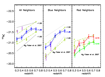
Figure 14.— ${}^{0.5}M_{r^{\prime}}^{*}$ as a function of redshift derived from Fig. 12 using three fixed $\alpha$. The dashed curve with triangles is the $M_{B}^{*}$ from Faber et al. (2007), and the one with crosses symbols is the ${}^{0.5}M_{r^{\prime}}$ by applying a simple color transfer from $B$ to $r^{\prime}$. The linear fits for the WiggleZ neighbor galaxies are overplotted as the dotted lines. The RCS-WSF sample is overplotted as purple open circle. The derived evolutionary term, i.e., the slope of the fit, is –1.31 for all the neighbors (the left panel), –2.10 with $\alpha$= –1.30 for the blue neighbors (the middle panel), and –1.59 for the red neighbors with $\alpha$=–0.40.

Table 3Parameters for Luminosity Functions of the WiggleZ Neighbors

All Neighbors
redshift	${}^{0.5}M_{r^{\prime}}^{*}$	$\alpha$
fitting $\alpha$
0.25–0.35	-21.46$\pm$0.18	-1.42$\pm$0.05
0.35–0.45	-21.33$\pm$0.21	-1.35$\pm$0.08
0.45–0.55	-20.89$\pm$0.14	-0.89$\pm$0.10
0.55–0.65	-21.23$\pm$0.15	-0.97$\pm$0.12
0.65–0.75	-21.10$\pm$0.16	-0.76$\pm$0.18
redshift	${}^{0.5}M_{r^{\prime}}^{*}$	${}^{0.5}M_{r^{\prime}}^{*}$	${}^{0.5}M_{r^{\prime}}^{*}$
	$\alpha$= -1.50	$\alpha$= -1.30	$\alpha$= -1.00
0.25–0.35	-21.68$\pm$0.11	-21.16$\pm$0.08	-20.60$\pm$0.06
0.35–0.45	-21.70$\pm$0.12	-21.22$\pm$0.09	-20.69$\pm$0.06
0.45–0.55	-21.92$\pm$0.10	-21.51$\pm$0.08	-21.02$\pm$0.05
0.55–0.65	-21.98$\pm$0.09	-21.65$\pm$0.07	-21.26$\pm$0.05
0.65–0.75	-21.89$\pm$0.08	-21.63$\pm$0.06	-21.30$\pm$0.05
Q	-0.64$\pm$0.32	-1.31$\pm$0.24	-1.95$\pm$0.19
${}^{0.5}M_{r^{\prime}}^{*}(z=0.5)$	-21.84$\pm$0.05	-21.44$\pm$0.04	-20.98$\pm$0.03
Blue Neighbors
redshift	${}^{0.5}M_{r^{\prime}}^{*}$	$\alpha$
fitting $\alpha$
0.25–0.35	-21.41$\pm$0.25	-1.56$\pm$0.06
0.35–0.45	-21.34$\pm$0.29	-1.49$\pm$0.10
0.45–0.55	-20.90$\pm$0.17	-1.02$\pm$0.11
0.55–0.65	-21.19$\pm$0.19	-1.05$\pm$0.15
0.65–0.75	-21.02$\pm$0.18	-0.74$\pm$0.21
redshift	${}^{0.5}M_{r^{\prime}}^{*}$	${}^{0.5}M_{r^{\prime}}^{*}$	${}^{0.5}M_{r^{\prime}}^{*}$
	$\alpha$= -1.50	$\alpha$= -1.30	$\alpha$= -1.00
0.25–0.35	-21.23$\pm$0.11	-20.76$\pm$0.08	-20.23$\pm$0.06
0.35–0.45	-21.34$\pm$0.13	-20.90$\pm$0.10	-20.40$\pm$0.07
0.45–0.55	-21.72$\pm$0.11	-21.32$\pm$0.09	-20.87$\pm$0.06
0.55–0.65	-21.80$\pm$0.10	-21.49$\pm$0.08	-21.13$\pm$0.06
0.65–0.75	-21.79$\pm$0.09	-21.55$\pm$0.07	-21.24$\pm$0.06
Q	-1.49$\pm$0.34	-2.10$\pm$0.26	-2.71$\pm$0.20
${}^{0.5}M_{r^{\prime}}^{*}(z=0.5)$	-21.58$\pm$0.05	-21.21$\pm$0.04	-20.78$\pm$0.03
Red Neighbors
redshift	${}^{0.5}M_{r^{\prime}}^{*}$	$\alpha$
fitting $\alpha$
0.25–0.35	-20.23$\pm$0.20	0.099$\pm$0.27
0.35–0.45	-20.74$\pm$0.22	-0.50$\pm$0.19
0.45–0.55	-20.60$\pm$0.20	-0.26$\pm$0.21
0.55–0.65	-21.21$\pm$0.24	-0.64$\pm$0.22
0.65–0.75	-21.33$\pm$0.38	-0.77$\pm$0.37
redshift	${}^{0.5}M_{r^{\prime}}^{*}$
	$\alpha$= -0.70	$\alpha$= -0.40
0.25–0.35	-20.51$\pm$0.12	-20.40$\pm$0.09
0.35–0.45	-20.96$\pm$0.10	-20.63$\pm$0.09
0.45–0.55	-20.99$\pm$0.09	-20.73$\pm$0.08
0.55–0.65	-21.28$\pm$0.09	-20.98$\pm$0.07
0.65–0.75	-21.26$\pm$0.11	-21.01$\pm$0.09
Q	-1.79$\pm$0.37	-1.59$\pm$0.30
${}^{0.5}M_{r^{\prime}}^{*}(z=0.5)$	-21.02$\pm$0.05	-20.76$\pm$0.04

Table 4Parameters for Luminosity Functions of the RCS-WSF Sample

All Neighbors
redshift	${}^{0.5}M_{r^{\prime}}^{*}$	$\alpha$
fitting $\alpha$
0.25–0.35	-21.04$\pm$0.08	-1.10$\pm$0.03
0.35–0.45	-21.05$\pm$0.10	-0.94$\pm$0.06
redshift	${}^{0.5}M_{r^{\prime}}^{*}$	${}^{0.5}M_{r^{\prime}}^{*}$	${}^{0.5}M_{r^{\prime}}^{*}$
	$\alpha$= -1.50	$\alpha$= -1.30	$\alpha$= -1.00
0.25–0.35	-22.14$\pm$0.07	-21.53$\pm$0.05	-20.81$\pm$0.03
0.35–0.45	-22.14$\pm$0.09	-21.67$\pm$0.06	-21.13$\pm$0.05
Blue Neighbors
redshift	${}^{0.5}M_{r^{\prime}}^{*}$	$\alpha$
fitting $\alpha$
0.25–0.35	-20.94$\pm$0.41	-1.52$\pm$0.03
0.35–0.45	-21.59$\pm$0.73	-1.55$\pm$0.06
redshift	${}^{0.5}M_{r^{\prime}}^{*}$	${}^{0.5}M_{r^{\prime}}^{*}$	${}^{0.5}M_{r^{\prime}}^{*}$
	$\alpha$= -1.50	$\alpha$= -1.30	$\alpha$= -1.00
0.25–0.35	-20.87$\pm$0.18	-20.30$\pm$0.13	-20.00$\pm$-0.0
0.35–0.45	-21.39$\pm$0.29	-20.82$\pm$0.21	-20.20$\pm$0.15
Red Neighbors
redshift	${}^{0.5}M_{r^{\prime}}^{*}$	$\alpha$
fitting $\alpha$
0.25–0.35	-20.52$\pm$0.09	-0.64$\pm$0.06
0.35–0.45	-20.81$\pm$0.09	-0.66$\pm$0.06
redshift	${}^{0.5}M_{r^{\prime}}^{*}$
	$\alpha$= -0.70	$\alpha$= -0.40
0.25–0.35	-20.62$\pm$0.04	-20.14$\pm$0.04
0.35–0.45	-20.86$\pm$0.04	-20.45$\pm$0.03

We adopt the parametrization of ${}^{0.5}M_{r^{\prime}}^{*}(z)=-21.44-1.31(z-0.5)$ from the ‘All’ sample in the derivation of the red-galaxy fraction in the following subsection.

4.6. The Fraction of Red Neighbors

In Figure 6 we have observed that dusty star-forming galaxies are not common for both the WiggleZ galaxies and their neighbors. The red neighbors of the WiggleZ galaxies are more likely to be those which have completed their star formation. We investigate the fraction of these red passive neighbors ($f_{red}$) as a function of redshift. We define red neighbor galaxies the same way as described in §4.5.1. The boundaries separating the blue and the red galaxies are shown in Fig. 11, which is about 0.27 mag bluer than the red-sequence, k-corrected to $z=0.5$. This color separation is equivalent to the gap in the galaxy bimodal color distribution at a fixed redshift seen in our samples. The fraction of net red neighbors to the total net neighbor counts as a function of redshift is presented in Fig. 15. We compute $f_{red}$ to four different depths of ${}^{0.5}M_{r^{\prime}}^{*}+\Delta M$ with ${}^{0.5}M_{r}^{*}$ as described in §4.5.3 and $\Delta M$=[0.0, 0.5, 1.0, 1.4], with the largest $\Delta M$ determined by the depth of sampling of the data from the largest redshift bin. The error in $f_{red}$ is estimated using Poisson statistics.

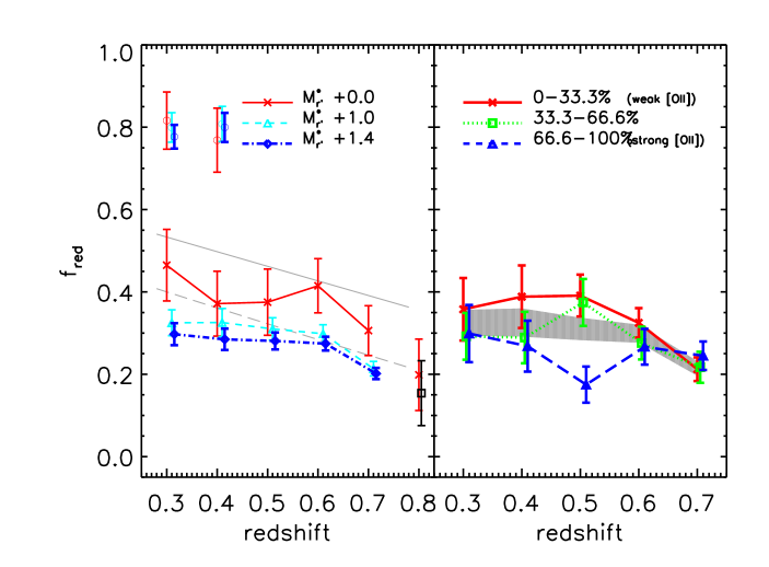
Figure 15.— Left: Fraction of red neighbors $f_{red}$ as a function of redshift to different $M_{r^{\prime}}$ depth. Different curves represent the $f_{red}$ computed using different magnitude depth as noted in the plot. The gray straight lines are from Iovino et al. (2010) for their Sample III ($<M^{*}+0.8$) ‘All’ (solid linestyle) and ‘Isolated’ (dashed linestyle) subsamples. The $f_{red}$ of the RCS-WSF sample at $z\sim$0.30 and 0.40 are overplotted as individual open symbols, which have a value of $\sim$0.8. The $f_{red}$ for the $z=0.75-0.85$, which is beyond the redshift range of our main sample, are plotted as individual points for magnitude limits of $M^{*}_{r^{\prime}}$ and $M^{*}_{r^{\prime}}+1.2$ (black square) to illustrate the continuous decrease of $f_{red}$ beyond $z\sim 0.7$. Right: $f_{red}$ computed using ${}^{0.5}M_{r^{\prime}}^{*}+1$ depth after controlling for the EW([OII]$\lambda$3727Å) of the WiggleZ markers. The gray shaded region is the $f_{red}$ using all markers with the same magnitude limit. The $f_{red}$ is similar regardless of the properties of the markers.

We observe that $f_{red}$ is not a strong function of redshift. Within the uncertainties of the measurements, $f_{red}$ can be described as flat between $z=0.25$ and 0.65, with an average of $\sim$0.28$\pm$0.01 for the magnitude limit of ${}^{0.5}M_{r^{\prime}}^{*}+1.4$ . At $z\sim 0.7$, there appears to be a drop in $f_{red}$ at $\sim 3.5\sigma$ level. We also see a relatively small change in $f_{red}$ within the relatively magnitude range we probed – changing by the order 0.1 over the 1.4 magnitude range, often within the uncertainties of the measurements in the same redshift bin. However, we note that differentially, as indicated by the GLFs of the red and blue galaxies, the fraction of blue galaxies increases significantly at the faint-end. Using data combining the two lowest redshift bins where we can sample down to ${}^{0.5}M_{r^{\prime}}^{*}+2.5$, we find $f_{red}$$\sim 0.22\pm 0.01$, a difference of $\sim 5\sigma$ from the $f_{red}$$\sim 0.45\pm 0.04$ measured at ${}^{0.5}M_{r^{\prime}}^{*}$.

For comparison, the $f_{red}$ for galaxies around the RCS-WSF sample of cluster galaxy markers are also plotted in Fig. 15, which have an average $f_{red}\sim 0.8$ for the $z\sim$0.3 and 0.4 bins. As expected, the $f_{red}$ for the RCS-WSF sample is much larger than that for the WiggleZ neighbors.

We also compute the $f_{red}$ values for subsamples of WiggleZ markers in different EW([OII]$\lambda$3727Å) bins. We divide the markers into three groups based on the 33.3 and 66.7 percentiles in the distribution of EW([OII]$\lambda$3727Å). The $f_{red}$ values, computed using the limit of ${}^{0.5}M_{r^{\prime}}^{*}+1$, as a function of redshift are presented in the right panel of Figure. 15. The gray shaded area is the $f_{red}$ calculated with the same magnitude limit using all the neighbors (i.e., the dashed blue curve in the left panel), overlaid for comparison. Although the WiggleZ markers with stronger EW([OII]$\lambda$3727Å) appear to have somewhat lower $f_{red}$, the $f_{red}$ for the different bins are well within the individual measurement uncertainties, with the exception of the $z=0.5$ bin. Averaging over all redshift bins, we find the mean $f_{red}$ for the three EW([OII]$\lambda$3727Å) bins, from low to high, to be $0.305\pm 0.019$, $0.278\pm 0.021$, and $0.246\pm 0.021$, or, a difference of about 2$\sigma$ between the weakest and strongest [OII]$\lambda$3727Å samples. Thus, there is some evidence that the neighbors of markers with the largest EW([OII]$\lambda$3727Å may have a lower average $f_{red}$, indicating regions around galaxies with large specific star-formation rates may have a larger fraction of star-formation galaxies. However, the relatively low significance difference (which comes mostly from the $z=0.5$ bin) is consistent with our conclusion of Figures 7 and 8 that the properties of the neighbors are not strongly dependent on the characteristics of the WiggleZ galaxies themselves.

5. Discussion

5.1. Robustness of Our Results

We have demonstrated that our novel approach – probing photometric properties of galaxies using color-color-magnitude cubes of neighbors around galaxies of known redshift – has yielded robust and interesting results. The advantages of our method are: (1) being straightforward, as it is equivalent to counting galaxies within an aperture and applying statistical background corrections; (2) not sensitive to whether the sample of the markers is complete; (3) allowing us to derive the photometric properties of galaxies to a limit considerably deeper than the corresponding limits for the spectroscopic sample; and (4) providing a complete census of the neighboring galaxies independent of the spectral/color properties of the galaxies. The key point in the method is the assumption that the marker galaxies and the excess galaxy counts around them are at the same redshift. The net neighbor counts around an individual galaxy are not statistically meaningful, but stacking color-color-magnitude cubes of a large number of markers provide statistically significant quantities. However, much care is required in carrying out the procedure.

First, proper background correction is essential in our method, especially when the signal of the net excess is only a fraction of the total galaxy counts. Any systematic discrepancy in the background subtraction would have a profound effect on the result. If the background is under-subtracted, the intrinsic properties of the net excess galaxies will be overwhelmed by the background counts; for instance, it may result in a power-law galaxy luminosity function without an apparent bend/knee. On the other hand, over-subtracting the background may result in small, or even negative, net counts, and hence no analyses can be done. The very large angular size of the RCS2 patches allows us to use photometric data from the same patch as the markers to estimate the background correction, minimizing any possible systematic issues. The use of uniform random catalogs to map out the imaging survey area, CCD chip gaps, bad CCD columns, bright star halos and other artifacts, ensure the proper treatment of the sampling aperture size. Our exercise of measuring excess counts centered on a large number of random positions in §2.2 demonstrates that we have handled the background correction properly, as the net excess around the randomly drawn points has a mean value of essentially zero and is not a function of galaxy magnitudes or colors.

Another way of verifying the robustness of our background subtraction technique is to use the WiggleZ redshift sample. While it poorly samples the whole photometric galaxy catalog, the very large sample of WiggleZ redshifts allows us to test the principle of background subtraction in general, and our technique in particular. We perform this test by comparing the ratio of the net excess galaxy counts to the total counts within the $r_{p}=0.25$Mpc aperture in both the photometric and WiggleZ redshift samples. We note that this method may not produce an exact comparison, as the WiggleZ sample has a number of selection criteria which may produce different selection effects for galaxies at different redshifts that are not possible to mimic using a purely magnitude-limited photometric sample. The most significant selection effect that produces a significant difference in the redshift distribution between a $r^{\prime}$-band selected sample and the WiggleZ sample is the low-redshift-rejection (LRR) applied to the selection of WiggleZ targets (see §2.3). Thus, we limit our comparison to using data from WiggleZ markers in the three high-redshift bins of our sample ($0.45<z<0.75$). For the photometric sample of counts of neigbors to the WiggleZ markers, we count only galaxies with $20<r^{\prime}<22.5$ (which is the WiggleZ optical-band selection criterion). For the WiggleZ galaxies, we count all WiggleZ glaxies within the aperture of each marker, and deem galaxies with a redshift within $0.002(1+z)$ of a marker galaxy as associated. We find the ratio of net excess counts to total counts in the aperture to be $0.193\pm 0.010$ for the photometric sample, where the uncertainty is based on Poisson statistics. For the equivalent ratio from the WiggleZ redshift sample, we obtain $0.196\pm 0.014$ (with 235 out of 1202 galaxies satisfying the redshift criterion). Thus, our statistical background subtraction technique produces net counts that are entirely consistent with results using a sample of galaxies with known redshifts, further adding confidence to the robustness of method.

Second, incorrect redshift measurements of the markers will dilute the results. The redshift plays the key role in computing the distance modulus, k-correction, and the aperture size for a fixed physical diameter. The first two impact directly on the rest-frame color and magnitude distributions of the neighbors. The latter affects the surface density of the excess counts. Since the redshift confidence for the markers with redshift quality flag $Q_{zspec}$=3 is $\sim$78.7%, we test the effect of incorrect redshift measurement by repeating our analyses using objects with $Q_{zspec}$=4 and 5 only, at the cost of having a weaker signal due to stacking fewer color-color-magnitude cubes. We find that the results are very similar to what we have presented here.

Finally, an interesting question is how often we have another WiggleZ galaxy within the aperture ($r_{p}$ = 0.25 Mpc) centered at a WiggleZ marker. We find that $\sim$5-10% of the markers have at least one other WiggleZ galaxy within a radius of 0.25 Mpc, but the percentage drops to $\sim$1% if these other WiggleZ galaxies have to be at a similar redshift ($\Delta z\leq 0.002(1+z)$) as the marker. The range in the percentage is patch dependent, as the number density of WiggleZ galaxies varies in different patches. We also find that the number of the enclosed WiggleZ galaxies is not a strong function of redshift. Therefore, we conclude that the properties of the WiggleZ neighbors should not be significantly contaminated by the WiggleZ galaxies themselves.

5.2. The WiggleZ Neighbor Galaxy Luminosity Function

5.2.1 The Schechter Function Fit

Our WiggleZ galaxy neighbor sample represents a complete census of galaxies in the neighborhood of star-forming galaxies over the redshift range of 0.25 to 0.75. On the color-magnitude plane, we separate the galaxy sample into red and blue galaxy subsamples. The GLFs for both the ‘Blue’ and ‘Red’ galaxy samples can be fitted very well with single Schechter functions. Based on the low-redshift bins, where there is sufficient depth to measure the faint-end slope unambiguously, they have different shapes such that the red galaxies have a dipping faint-end (best fitted with $\alpha\lower 0.43057pt\hbox{\hbox to0.0pt{\raise 2.58334pt\hbox{\hskip 1.29167pt{{$\scriptscriptstyle>$}}}\hss} \kern-1.72218pt{{$\scriptscriptstyle\sim$}}}-0.6$), whereas the blue galaxies have a steep rising faint-end which is best fitted with $\alpha\sim-1.3$. This is similar in general to what is seen in clusters, where red-sequence galaxies typically have a turn over in the GLF, while the blue galaxies increase in number steeply at the faint end (e.g., Barkhouse et al., 2007; Wolf et al., 2009).

We can make a direct comparison between the WiggleZ neighbor sample, representing galaxies associated with star-forming galaxies, and the neighbors of the RCS-WSF sample, representing galaxies in dense cluster environments, by combining the $z\sim 0.3$ and 0.4 subsamples. We find the ‘Blue’ galaxy samples to have essentially identical GLF parameters: $\alpha=-1.42\pm 0.08$ and $-1.57\pm 0.13$, and ${}^{0.5}M_{r}^{*}=-21.15\pm 0.19$ and $-21.37\pm 0.47$. The red galaxy GLFs for the two samples appear to have different faint-end slopes at the $4.3\sigma$ level, with $\alpha=-0.18\pm 0.17$, and $-0.74\pm 0.06$ for the WiggleZ neighbors and the RCS-WSF neighbors. The RCS-WSF red galaxy neighbors also have a marginally brighter ${}^{0.5}M_{r}^{*}$ of $-20.78\pm 0.09$, compared to $-20.42\pm 0.15$ for the WiggleZ neighbor sample, at the $2\sigma$ level. However, this difference is most likely a reflection of the different $\alpha$ used in the best fits; fitting both ‘Red’ GLFs using a common $\alpha=-0.5$ for $z=0.25$ to 0.45, we obtained ${}^{0.5}M_{r^{\prime}}^{*}$=$-20.42\pm 0.09$ and $-20.53\pm 0.07$ for the RCS-WSF and the WiggleZ neighbor sample, respectively. We will further discuss the difference in the GLF shape in §5.4.

5.2.2 The Evolution of the Galaxy Luminosity Function

We use the parameter $Q$ (see $\S$4.5) to measure the evolution of $M^{*}$, with the asssumption of $\alpha$ being constant with redshift for the faint-end of the GLF. The results for different samples and $\alpha$’s are shown in Fig. 14. There is a general brightening of $M^{*}$ with larger redshift. An intereting trend is that that red-sequence galaxies may have a lower $Q$ value than that of blue-cloud galaxies, $\sim-1.6$ versus $\sim-2.1$, but only at the 1.3$\sigma$.

Using a sample drawn from the DEEP2 and COMBO-17 data and with SDSS data as the local universe epoch, Faber et al. (2007) studied the evolution of the GLF in the redshift range of $0.1\leq z<1$ in the $M_{B}$ band, which is similar in rest wavelength to our ${}^{0.5}M_{r^{\prime}}$ band. They obtained $Q$ values of $-1.23\pm 0.36$, $-1.34\pm 0.22$, $-1.20\pm 0.21$, over the range of $z\sim 0$ to $1$, for their ‘All’, ‘Blue’, and ‘Red’ samples. These values appear to be lower from those derived in our samples (see Table 3) at moderately significant levels, especially for the ‘Blue’ sample. However, the comparison is much more similar if we limit their data to the same redshift range as ours. In Figure 14, we plot their $M_{B}^{*}$ data points. For a more direct comparison, we also convert their $B$ band to our ${}^{0.5}M_{r^{\prime}}$ by applying color corrections based on $B-r^{\prime}$ colors from GISSEL (Bruzual & Charlot, 2003) to convert $M_{B}$ to $M_{r^{\prime}}$ at zero redshift, and then k-correct $M_{r^{\prime}}$ to ${}^{0.5}M_{r^{\prime}}$. These data are also plotted in Figure 14.

We refit the $Q$ factor from Faber et al. (2007) using their data within the redshift range covered by our the WiggleZ neighbor sample. We find $Q=$ [$-1.45\pm 0.25,-2.02\pm 0.32,-0.67\pm 0.38$] (in their $B$ band) for their ‘All’, ‘Blue’, and ‘Red’ samples, respectively, compared to our values of $-1.31\pm 0.24$, $-2.10\pm 0.26$ ($\alpha$=-1.3) and $-1.59\pm 0.30$ ($\alpha=-0.4$) in Table 3. Thus, the derived $Q$ values from the two studies over the same redshift range are similar, especially for the ‘All’ and ‘Blue’ samples. For the ‘Red’ samples, the WiggleZ neighbors have a steeper evolution, at the $\sim 2\sigma$ level. We note that over this redshift range the Faber et al. results also produce a relatively significant lower $Q$ value for their ‘Red’ sample compared to that for their ‘Blue’ sample, at the 2.7$\sigma$ level, reinforcing a possible similar trend in the WiggleZ samples. The marginally steeper evolution of the ‘Red’ samples in the two data sets could be a reflection of the difference in the selection for the red galaxy samples. This possible discrepancy could be an indication that there is a difference in the evolution of early-type galaxies based on the environment. The red galaxies in the WiggleZ neighbor sample are primarily in low density regions, conducive to star-formation; while those in the Faber et al. sample include red galaxies in all environments, with an expected bias towards high density regions. Thus, it is perhaps not surprising that the two samples have different $Q$ values, with the red GLF in low-density regions evolving more rapidly. However, we note that the differences discussed in this subsection are at the $\sim 2\sigma$ levels. Considerably more detailed studies are need to firmly establish the differences in the evolution of the GLF of different galaxy populations in different environments.

5.3. The Red-Galaxy Fraction

When the star forming activity in a galaxy ceases, the galaxy ought to become redder in colors. In Fig. 15 we explore the redshift dependence of the red galaxy fraction, $f_{red}$. Since the dependence of $f_{red}$ on $z$ is similar for samples of different depths, for the remainder of the analysis, we use the ${}^{0.5}M_{r^{\prime}}$$<$${}^{0.5}M_{r^{\prime}}^{*}+1.4$ sample. which has $f_{red}$ measurements with the smallest error bars and is complete for all the redshift bins, unless noted otherwise.

5.3.1 The Redshift Dependence of $f_{red}$

We observe that $f_{red}$ is remarkably similar at $0.25\leq z<0.65$, with a value of $\sim 0.28$. A linear fit to the 4 points gives a slope of $-0.070\pm 0.098$. The $f_{red}$ drops to about 0.20 for the $z=0.7$ bin. This drop, between the $z=0.6$ and 0.7 bins, is statistically significant at the $\sim 3.5\sigma$ level. If we assume the best linear fit for $f_{red}$ from the four data points with $z<0.65$, the $f_{red}$ at $z=0.7$ is 4.8$\sigma$ below the extrapolation from the fit. An alternative simpler description of the trend is a linear decrease; however, this linear fit, to all 5 points, has a reduced $\chi^{2}$ of 3.1, indicating that it is not a good description of the data.

To investigate whether there is a change in the dependence of $f_{red}$ on $z$ at $z\sim 0.7$, we extend the measurement of $f_{red}$ to $z\sim 0.8$. The WiggleZ sample has a large number of galaxies at $0.75<z<0.85$, which we have not included in our analysis because the RCS2 photometry is only complete to a relatively shallow absolute magnitude limit of –20.6. Nevertheless, this bin is complete to ${}^{0.5}M_{r^{\prime}}$+1.2, and hence, we perform the same analysis using the 5819 WiggleZ galaxies in this redshift bin as markers. The $f_{red}$ computed using this sample is plotted on Figure 15. It shows a continuous drop from the $z=0.7$ data point. A linear fit applied to all 6 data points from $z=0.3$ to $z=0.8$ with a limiting magnitude of $M^{*}+1.2$, produces a reduced $\chi^{2}$ of 6.3, indicating a poor fit. Thus, the addition of the higher redshift data adds confidence to the conclusion there is an on-set of a significant drop in the red-galaxy fraction at $z>0.65$.

We compare our results to Iovino et al. (2010), who derived the blue galaxy fraction $F_{blue}$ for galaxy samples in different environments from the zCOSMOS survey. Of particular interest is their ‘All’ and ‘Isolated’ subsamples of Sample III, with a depth of $M=M^{*}+1.5$, covering the redshift range of $\sim 0.2$ to 0.6. Iovino et al. (2010) parametrize the evolution of $F_{blue}$ by a power law of the form equivalent to: $f_{red}$$(z)=1-F_{blue}(0)(1+z)^{\beta}$, with $F_{blue}(0)=0.58\pm 0.10$ and $\beta=0.69\pm 0.44$ for the Isolated sample, using 3 data points. We plot their $F_{blue}(z)$ as $f_{red}$ on Figure 15 using their parametrization. Our $f_{red}$ has values more similar to their Isolated sample, and well below their ‘All’ sample. This is consistent with our expectation that the WiggleZ neighborhoods have by-and-large a low galaxy density environment, dominated by star-forming galaxies.

For a more direct comparison, we fit our $f_{red}$ with the power law over a longer redshift range ($z=0.20-0.70$) than Iovino et al. (2010), and obtain (for $M^{*}+1.4$): $F_{blue}(0)=0.59\pm 0.04$, and $\beta=0.52\pm 0.13$ with a reduced $\chi^{2}\sim 3.1$. Thus, our data show a similar, rate of decrease of $f_{red}$ with increasing redshift as that found by Iovino et al. (2010). However, we note that both of the fitting models to our data–the linear fit and the power-law fit–have reduced $\chi^{2}$s considerably larger than 1: $\sim 3-4$ for both using data up to $z=0.7$ and $z=0.8$. This indicates that a simple continuous decrease of $f_{red}$ with redshift is likely not a good description of its evolution.

Thus, an interesting result is that our data, covering a longer redshift baseline than the Iovino et al. (2010) study, show a more or less constant $f_{red}$ up to $z\sim 0.6$ before seeing a drop. Such a description of the change in $f_{red}$ for galaxies in poor environments with redshift is in fact also consistent with the data of the ‘Isolated’ sample of Iovino et al. (2010), with their three $F_{blue}$ data points covering the redshift between 0.2 and 0.6 being consistent with having similar values within their uncertainties. We note that the more or less constant $f_{red}$$\sim 0.3$ for $z\lower 0.43057pt\hbox{\hbox to0.0pt{\raise 2.58334pt\hbox{\hskip 1.29167pt{{$\scriptscriptstyle<$}}}\hss} \kern-1.72218pt{{$\scriptscriptstyle\sim$}}}0.6$ for the WiggleZ neighbor samples is similar to that obtained for galaxies in low-density regions at the local universe at $z\sim 0$; e.g., Balogh et al. (2004) derived $f_{red}\sim 0.35$ from the SDSS sample for their low local-galaxy density samples of galaxies of $M_{V}\lower 0.43057pt\hbox{\hbox to0.0pt{\raise 2.58334pt\hbox{\hskip 1.29167pt{{$\scriptscriptstyle<$}}}\hss} \kern-1.72218pt{{$\scriptscriptstyle\sim$}}}-20$. The $f_{red}$ for the WiggleZ galaxy neighbors extrapolate to $\sim 0.32$ at $z=0$. Thus, there appears to be a relatively small amount of evolution in $f_{red}$ in low galaxy density regions from $z\sim 0.6$ all the way to $z\sim 0$.

Because the WiggleZ sample is selected in part by observed UV and optical fluxes of the objects, this abrupt increase in the change in $f_{red}$ between the 0.6 and 0.7 redshift bins could conceivably be contributed by some unknown correlation or thresholding effect between the star-formation rate or luminosity of the markers and the properties of their neighbors. To test the effect of the UV flux selection criterion, we select two subsamples of markers within an identical UV absolute luminosity range which is complete in the both $z\sim 0.6$ and $z\sim 0.7$ bins ($M_{NUV}\leq-20.7$), and compute their $f_{red}$. We obtain $f_{red}$=0.293$\pm$0.022, and 0.207$\pm$0.017 for the neighbors in the two redshift bins, indicating a similar and significant (at $\sim 3\sigma$) drop to that when the whole sample without control on $M_{NUV}$ is used. Similarly, we compare the $f_{red}$ of neighbors of subsamples of markers with the same $r^{\prime}$ absolute magnitude (${}^{0.5}M_{r^{\prime}}$ between –21.5 and –22.5) in the last two redshift bins, and obtain $f_{red}$=0.255$\pm$0.045 and 0.176$\pm$0.033; again, showing a drop similar to that obtained using the whole redshift bins. Thus, we can conclude that the drop in $f_{red}$ between $z\sim 0.6$ and 0.7 is likely not a result of the different star-formation properties of the central markers.

5.3.2 The Evolution of the Red-Galaxy Fraction

Our data allow us to look at the redshift evolution of the red-galaxy fraction $f_{red}$ up to $z\sim 0.7$ using samples complete to an absolute luminosity about 1.5 mag beyond $M^{*}$. Under the simplest assumption of a sample of galaxies in a closed volume, $f_{red}$ allows us to follow the end result of the process of galaxies having their star formation quenched and eventually turning red, becoming a member of the red sequence (e.g., Kodama & Bower, 2001). However, the use of a luminosity limit produces ambiguities in how to interpret the average change in the galaxy population between the different epochs, since galaxies of a given mass may enter and leave the sample depending on their star-formation state. To assist in the interpretation of the observed change in $f_{red}$ with redshift, we illustrate in Figure 16 the possible flows of galaxies into and out of luminosity-limited blue and red galaxy samples.

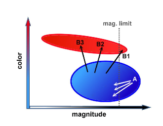
Figure 16.— Schematic color-magnitude diagram showing the flows of galaxies into and out of the blue cloud. The narrow red ellipse represents the location of the red sequence; the blue ellipse marks the blue cloud. The vertical dotted line indicates the magnitude limit of the sample for computing $f_{red}$. The white arrows (A) show the replenishment of galaxies in the blue cloud due to an increase in the star-formation rate of blue galaxies fainter than the magnitude limit. The black three arrows illustrate the possible flows of galaxies from the blue cloud into the red-sequence after star formation quenched. Arrow B3 represents star-formation being quenched by an approximately equal-mass merger. Arrow B2 stands for the quenching of star formation, while arrow B1 represents the case when the galaxy moves back beyond the magnitude limit again due to its quenched star formation.

In a simple picture, the number of galaxies in the blue cloud can be augmented by new star formation in galaxies fainter than the luminosity limit, boosting them into the sample, adding to the blue galaxy counts. This replenishment is represented by the white arrows (A) in Figure 16. In a field situation, where infall in general is not a major process, one can consider this replenishment generally being controlled by the canonical down-sizing scenario of star formation – lower mass galaxies may start forming stars, and in some instances, boosting the luminosity of the galaxy into the blue cloud sample.

On the other hand, one would expect a continuous flow of galaxies from the blue cloud into the red sequence as galaxies evolve. This would primarily be created by the quenching of star formation in galaxies in the blue cloud by various processes. There are several paths that this transformation into the red sequence may take, and the are illustrated by the black three arrows (B1, B2, and B3) schematically. The luminosity of a galaxy will generally fade as its star formation is quenched and turns red (B1 and B2), and some of them will become fainter than the sample magnitude limit and leave the sample. There is also a possibility that the galaxy becomes brighter if the cessation of star formation follows a major merger (arrow B3). However, in poor environments, it is unlikely that this is a dominant event; e.g., Hsieh et al. (2008) found approximately 6% of galaxies may have undergone a major merger since $z\sim 0.8$.

In the WiggleZ sample of neighbors of strong star-forming galaxies we find that $f_{red}$ is essentially flat from $z\sim 0.6$ to the present, with evidence of a decrease at $z\lower 0.43057pt\hbox{\hbox to0.0pt{\raise 2.58334pt\hbox{\hskip 1.29167pt{{$\scriptscriptstyle>$}}}\hss} \kern-1.72218pt{{$\scriptscriptstyle\sim$}}}0.6$. In the simplest picture, the change in $f_{red}$ over redshift can be interpreted as a change in the relative flow rates of galaxies into the red sequence and into the blue cloud. Thus, at $z\lower 0.43057pt\hbox{\hbox to0.0pt{\raise 2.58334pt\hbox{\hskip 1.29167pt{{$\scriptscriptstyle<$}}}\hss} \kern-1.72218pt{{$\scriptscriptstyle\sim$}}}0.6$ we can effectively conclude that the rate of transformation of blue galaxies into red galaxies, which builds up the red-sequence, is approximately equal to the replenishment rate of blue galaxies brighter than the sampling limit; while at $z\lower 0.43057pt\hbox{\hbox to0.0pt{\raise 2.58334pt\hbox{\hskip 1.29167pt{{$\scriptscriptstyle>$}}}\hss} \kern-1.72218pt{{$\scriptscriptstyle\sim$}}}0.6$ the rate of transformation of blue galaxies into red galaxies is lower than the replenishment rate of blue galaxies, so that there is a net decrease of red galaxies relative to the blue galaxies.

However, the change in $f_{red}$ with redshift does not give us unambiguous information on the actual changes in these rates. If we assume that the rate of the build-up of the red sequence is constant over the redshift range of $\sim 0.8$ to 0.2, we would then conclude that the rate of replenishment of blue galaxies (into the luminosity limited sample) is decreasing from $z\sim 0.8$ to 0.6, and then becomes stable, or decreasing at a much lower rate, at $z\lower 0.43057pt\hbox{\hbox to0.0pt{\raise 2.58334pt\hbox{\hskip 1.29167pt{{$\scriptscriptstyle<$}}}\hss} \kern-1.72218pt{{$\scriptscriptstyle\sim$}}}0.6$. Alternatively, if we assume that the replenishment of blue galaxies is constant, then the rate of transformation of blue cloud galaxies into the red sequence is increasing from $z\sim 0.8$ to 0.6, and become stable at $z\lower 0.43057pt\hbox{\hbox to0.0pt{\raise 2.58334pt\hbox{\hskip 1.29167pt{{$\scriptscriptstyle<$}}}\hss} \kern-1.72218pt{{$\scriptscriptstyle\sim$}}}0.6$. The detailed picture is certain to be more complex. In a more general picture, the environment will be a major factor that affects these rates of flows. An important effect to consider is the infall of galaxies into a high density region such as the parent halo of a galaxy cluster or group. We will discuss this effect in §5.4, in conjunction with the evolution of $f_{red}$ in clusters.

5.3.3 The $f_{red}$ of the Cluster Neighborhood Sample

We have also derived $f_{red}$ for the RCS-WSF cluster neighborhood sample for the $z\sim 0.3$ and $z\sim 0.4$ bins, which are plotted as open circles in Fig. 15. They show a clear difference due to the environments of the galaxies; the cluster neighborhood samples have $f_{red}$ of $\sim 0.8$, indicative of high galaxy density regions. While we do not have the redshift range to examine the evolution of $f_{red}$ in clusters, studies using similar techniques of large samples of clusters show a continuous decrease of $f_{red}$ with redshift, i.e., the Butcher-Oemler effect (Butcher & Oemler, 1984). For instances, Loh et al. (2008), using a sample of approximately 1000 clusters from RCS1 at $0.4\leq z\leq 0.9$, show a steady decrease in $f_{red}$ of about 0.4; while the spectroscopic sample of Ellingson et al. (2001) indicates a steady drop of $f_{red}$ from 0.9 to 0.7 at $z$=0.2-0.5.

Comparing these results with the WiggleZ neighbor sample, there appears to be a rather different behavior in the change in $f_{red}$ as a function of redshift for galaxies in regions around star-forming galaxies from those in high galaxy density regions around massive halos. Instead of a steady decline in $f_{red}$ with increasing redshift, the $f_{red}$ for the WiggleZ neighbors have a basically flat dependence on $z$, and show a significant drop only at $z\lower 0.43057pt\hbox{\hbox to0.0pt{\raise 2.58334pt\hbox{\hskip 1.29167pt{{$\scriptscriptstyle>$}}}\hss} \kern-1.72218pt{{$\scriptscriptstyle\sim$}}}0.65$. Similarly, Iovino et al. (2010) show that galaxies classified as being in a group environment have a much steeper dependence of their blue-galaxy fraction on redshift than those considered to be in isolated environments. This difference in the evolution of $f_{red}$ can be considered as a clear demonstration of the effect of environment on the evolution timescale of galaxy populations.

5.4. Galaxy Evolution and Environment

The topic of galaxy evolution has been studied in galaxy clusters over many decades. With modern large surveys, the focus has extended to field galaxies. Here, we would like to use the term ‘field’ to refer to all galaxies in a general blind field survey, such as SDSS or 2dF, where galaxy density ranges from that of isolated galaxies to clusters. Studies using such ‘field’ samples have revealed a strong correlation between many properties of galaxies and environment (usually parametrized by local galaxy density). One example is that the fraction of star-forming (or passively evolving galaxies) changes strongly with local galaxy density (e.g., Baldry et al., 2006; Li et al., 2009; Iovino et al., 2010). Other works focus on star-forming galaxies. These star-forming galaxies naturally reside in regions beyond galaxy clusters. Their star-formation rates and colors are found not to have a strong dependence on environment (e.g., Carter et al., 2001; Rines et al., 2005; Balogh et al., 2009; Cassata et al., 2007). Such conclusions appear to be different from the results from using all ‘field’ galaxies, and this is likely a reflection of the sample properties.

Our WiggleZ galaxies are members of these star-forming galaxies, selected by their detectable UV flux. We use the term ‘WiggleZ neighborhood’ to refer to local regions around the WiggleZ galaxies to distinguish it from the general ‘field’ environment. The WiggleZ neighborhood is likely low-density environment regions in the large-scale structure. The galaxy sample generated by counting excess galaxies in the WiggleZ galaxy neighborhood represents a census of galaxies in regions around star-forming galaxies covering a significant redshift range.

We also examine $f_{red}$ in dense environments using the neighbors of the RCS-WSF sample of cluster galaxies. The much higher $f_{red}$ value ($\sim 0.8$ vs $\sim 0.3$) measured is an indication of the more rapid build-up of the red sequence in dense environments. Furthermore, it appears that the evolution of $f_{red}$ for these two samples is also very different, with the WiggleZ neighbors having very moderate or no increase in $f_{red}$ since $z\sim 0.6$.

In the context of the discussion of Figure 16 in §5.3.2, the flow paths and rates of blue and red galaxies on the CMD in cluster environments would be very different from those in the WiggleZ neighborhoods. Here, the major source of replenishment of blue galaxies in massive dense halos is likely to be the infall of galaxies along the large-scale structure. These galaxies are then transformed into red galaxies within some time scale due to processes such as tidal striping, ram pressure, galaxy harassment and interactions, which are generally associated with the quenching of star formation in galaxy groups and clusters. The continuous increase in $f_{red}$ can also be in part attributed to the cosmological decrease in infall rate with time in a low $\Omega_{m}$ universe (e.g., Ellingson et al., 2001).

There is an additional difference between these two samples in the shape of the GLF of the red galaxy population. The Schechter function fit indicates that the red galaxies in dense environments have a GLF with a steeper faint-end. This can also be a result of the red sequence in cluster environments being in a more advanced build-up stage, or, the build-up of the faint-end of the red sequence in dense environment is more rapid than that in regions around star-forming galaxies. The build-up of the faint-end of the red sequence in clusters has been traced by a number of studies (e.g., Bell et al., 2004; Tanaka et al., 2005; Willmer et al., 2006; Stott et al., 2007; De Lucia et al., 2009). Gilbank et al. (2008) show some preliminary evidence that this build-up is faster in rich clusters than in poor clusters, which is consistent with the comparison here between clusters and low galaxy density regions. Another apparent difference in the GLF of the red galaxies in the two sample is that the red galaxies in the cluster sample show a significant excess to the Schechter function fit at bright magnitudes, suggesting that there are relatively more massive red galaxies in dense environments, either due to initial galaxy formation history or an increased rate of mergers in the evolution of these galaxies.

The possible difference in the evolution of $M^{*}$ of the red galaxy GLFs described in §5.2.2, while not of high statistical significance, also fits in with the scenario of the dependence of the evolution of the red galaxy population with environment. The lower value of $Q$ (i.e., slower evolution of $M^{*}$) for the Faber et al. (2007) ‘Red’ galaxy sample, which are in an environment denser than those from the WiggleZ sample, suggests that red galaxies in denser environments are likely older. This would be expected if galaxies in dense environments such as clusters and group turn red and dead earlier in the history of the universe than those in low-density region.

In summary, in the general scenario of galaxy evolution and its connection to the environment the WiggleZ neighborhoods can be considered as regions where there are minimal major environmental events affecting the evolution of galaxies. These regions are likely the low galaxy density parts of the large cosmic structure where star formation is still occurring well into the current epoch. Here, galaxies are unlikely to be affected by environmental influences that are associated with infall into a massive halo such as a substantial galaxy group or cluster. The galaxies in these neighborhoods can be considered as primarily following a secular galaxy evolution path, controlled by their own nature at birth, with environmental effects playing a role over a much longer time scale. In these environments, only a small fraction ($\sim$20-30%) of the galaxies have turned red over the redshift range of 0.7 to 0.3. In a cluster region, where there is a continuous infall of galaxies from the lower-density environments replenishing the blue cloud, the effects of the large dark matter parent halo on galaxies would produce a very different mix of galaxy populations. In these regions, environment plays a dominant role, accelerating the quenching of star formation, and transforming the infallen galaxies into the red sequence over a relatively short time scale, producing a red sequence in a more advanced evolutionary stage.

6. Summary

We have probed galaxy evolution at $0.25\leq z\leq 0.75$ using optical data from the RCS2 around $\sim$41,000 star-forming spectroscopic galaxies from the WiggleZ project. Because of the complicated selection criteria in the WiggleZ survey, galaxies in the spectroscopic sample have discrete characteristics as a function of redshift. We therefore examine optical properties of galaxies within 0.25 Mpc to WiggleZ galaxies using stacked color-color-magnitude cubes. The idea is to use the WiggleZ galaxies as markers, and assume that they and the surrounding neighbors are at the same redshift. By applying background subtraction and stacking the net excess counts over a large number of markers, we are able to study the properties of the neighbors around the WiggleZ galaxies.

We also examine how the optical colors of the neighbors correlate with the WiggleZ [OII]$\lambda$3727Å equivalent width, $NUV$ flux, and AGN activity indicators at different redshifts (Figures 7, 8, and 10). We find in general that the neighbor galaxies populate the same color-color spaces without significant dependence on these properties of the markers, suggesting that the properties of the neighbor galaxies are not strongly affected by, or correlate with, the characteristics of the WiggleZ galaxies themselves, Thus, they can be used to study the evolution of the photometric properties of galaxies in low-density, star-forming regions over the redshift range of 0.25 to 0.75.

Our major findings are:
(1) The majority of WiggleZ neighbors are blue galaxies which have a steeper faint-end slope and a faster evolution term in ${}^{0.5}M^{*}_{r^{\prime}}$ than the red galaxies.

The CMD of the WiggleZ neighbors shows the characteristic bimodal distribution of a red sequence and a blue cloud, with the latter dominating the galaxy population, containing 65 to 85% of the galaxies (depending on the depth of sampling and redshift). The GLFs of the two populations can be fitted with single Schechter functions, with the blue galaxies having a much steeper ($\alpha\sim-1.3$) faint-end than the red galaxies ($\alpha\sim-0.4$). Based on the three low-redshift bins ($0.25<z<0.55$), where the data are complete to ${}^{0.5}M_{r^{\prime}}$=–19.0, we find no significant changes in the faint-end slope of the GLFs with redshift. There is significant evolution in $M^{*}$ for both the ‘Blue’ and ‘Red’ subsamples. We find that blue galaxies have a marginally more rapid evolution in $M^{*}$ over this redshift range with $Q\sim-2.10$, compared to $Q\sim-1.59$ for the red galaxies. While the $Q$ values for both the red and blue galaxy samples appear to be steeper than the typical values in the literature, these evolution factors are similar to those from Faber et al. (2007) when compared over the same redshift range.

(2) The red galaxy fraction $f_{red}$ in the WiggleZ neighborhood is approximately constant since $z\sim 0.6$, but drops at $z\lower 0.43057pt\hbox{\hbox to0.0pt{\raise 2.58334pt\hbox{\hskip 1.29167pt{{$\scriptscriptstyle>$}}}\hss} \kern-1.72218pt{{$\scriptscriptstyle\sim$}}}0.7$.

The WiggleZ neighbor galaxies have a red-galaxy fraction ($f_{red}$) considerably smaller than that of the neighbors of the RCS-WSF sample of markers, at $0.25<z<0.45$, obtained the same way as the WiggleZ sample. The evolution of the WiggleZ neighbor $f_{red}$ with redshift is modest; $f_{red}$ can be described as basically flat as a function of redshift with only a very moderate decrease up to $z\sim 0.6$. The average $f_{red}$ value over the redshift range of $0.25<z<0.65$ is $\sim 0.30$, similar to field galaxies at $z\sim 0$. A large drop to $f_{red}$$\sim 0.20$ is seen for the $z\sim 0.7$ sample. This drop is confirmed by extending the measurement of $f_{red}$ to $z\sim 0.8$ using a sample with a slightly brighter absolute magnitude limit. Furthermore, this drop does not seem to be associated with the larger average luminosity of the markers at the higher $z$ bin. The change in $f_{red}$ with redshift in the WiggleZ neighborhood can be seen as either a higher rate of relatively bright ($M\lower 0.43057pt\hbox{\hbox to0.0pt{\raise 2.58334pt\hbox{\hskip 1.29167pt{{$\scriptscriptstyle<$}}}\hss} \kern-1.72218pt{{$\scriptscriptstyle\sim$}}}M^{*}+1$) star-forming galaxies entering the luminosity limited sample at $z\sim$0.7, or a decrease in the quenching rate of star formation at this redshift.

(3) The comparison between the WiggleZ and RCS-WSF neighbor samples shows an environmental influence on galaxy properties and evolution, with the red sequence in cluster environment being in a more advanced build-up stage.

We examine the effects of environment on the galaxy population properties by comparing the WiggleZ neighborhood galaxies to that of the RCS-WSF neighbor sample. Besides the expected and obvious difference in $f_{red}$ values of the two samples (with $f_{red}$, at $\sim 0.8$, being much larger in the RCS-WSF sample), we also find significant difference in the GLFs of the red galaxies of the two samples. The faint-end slope $\alpha$ for the red GLF of the RCS-WSF sample is considerably steeper ($\sim-0.7$ vs $\sim-0.4$). This can be taken as the build-up of the faint-end of the red sequence being in a more advanced stage in rich environments (such galaxy clusters and groups) than that in lower galaxy density regions around star-forming galaxies. Furthermore, there is also evidence that there are excess luminous red galaxies in the RCS-WSF sample. These findings point to the importance of environment in affecting the history of star formation in galaxies. Galaxies in cluster/group environments likely have suffered significant environmental events that rapidly shut down their star formation, turning the galaxy red. Whereas in regions where star formation is still prevalent, environmental events likely occur much less frequently and their effects spread over a longer time scale, delaying the build-up of the red sequence.

References

- Adelman-McCarthy et al. (2006) Adelman-McCarthy et al., J. K. 2006, ApJS, 162, 38
- Baldry et al. (2006) Baldry, I. K., Balogh, M. L., Bower, R. G., Glazebrook, K., Nichol, R. C., Bamford, S. P., & Budavari, T. 2006, MNRAS, 373, 469
- Baldwin et al. (1981) Baldwin, J. A., Phillips, M. M., & Terlevich, R. 1981, PASP, 93, 5
- Balogh et al. (2004) Balogh, M. L., Baldry, I. K., Nichol, R., Miller, C., Bower, R., & Glazebrook, K. 2004, ApJ, 615, L101
- Balogh et al. (1997) Balogh, M. L., Morris, S. L., Yee, H. K. C., Carlberg, R. G., & Ellingson, E. 1997, ApJ, 488, L75+
- Balogh et al. (2009) Balogh et al., M. L. 2009, MNRAS, 398, 754
- Barkhouse et al. (2007) Barkhouse, W. A., Yee, H. K. C., & López-Cruz, O. 2007, ApJ, 671, 1471
- Barnes & Hernquist (1991) Barnes, J. E. & Hernquist, L. E. 1991, ApJ, 370, L65
- Bell et al. (2004) Bell et al., E. F. 2004, ApJ, 608, 752
- Bertelli et al. (1994) Bertelli, G., Bressan, A., Chiosi, C., Fagotto, F., & Nasi, E. 1994, A&AS, 106, 275
- Blake et al. (2011) Blake, C., 2011, MNRAS, 415, 2892
- Blanton (2006) Blanton, M. R. 2006, ApJ, 648, 268
- Blanton et al. (2003) Blanton et al., M. R. 2003, ApJ, 594, 186
- Bongiorno et al. (2010) Bongiorno et al., A. 2010, A&A, 510, A56+
- Bruzual & Charlot (2003) Bruzual, G. & Charlot, S. 2003, MNRAS, 344, 1000
- Butcher & Oemler (1984) Butcher, H. & Oemler, Jr., A. 1984, ApJ, 285, 426
- Cannon et al. (2006) Cannon et al., R. 2006, MNRAS, 372, 425
- Carter et al. (2001) Carter, B. J., Fabricant, D. G., Geller, M. J., Kurtz, M. J., & McLean, B. 2001, ApJ, 559, 606
- Cassata et al. (2007) Cassata et al., P. 2007, ApJS, 172, 270
- Chabrier (2003) Chabrier, G. 2003, PASP, 115, 763
- Christlein et al. (2009) Christlein, D., Gawiser, E., Marchesini, D., & Padilla, N. 2009, MNRAS, 400, 429
- Colless et al. (2001) Colless et al., M. 2001, MNRAS, 328, 1039
- Cooper et al. (2007) Cooper et al., M. C. 2007, MNRAS, 376, 1445
- De Lucia et al. (2009) De Lucia, G., Poggianti, B. M., Halliday, C., Milvang-Jensen, B., Noll, S., Smail, I., & Zaritsky, D. 2009, MNRAS, 400, 68
- De Robertis et al. (1998) De Robertis, M. M., Yee, H. K. C., & Hayhoe, K. 1998, ApJ, 496, 93
- Dressler & Gunn (1983) Dressler, A. & Gunn, J. E. 1983, ApJ, 270, 7
- Dressler et al. (1980) Dressler et al., A. 1980, ApJ, 236, 351
- Drinkwater et al. (2010) Drinkwater et al., M. J. 2010, MNRAS, 401, 1429
- Ellingson et al. (2001) Ellingson, E., Lin, H., Yee, H. K. C., & Carlberg, R. G. 2001, ApJ, 547, 609
- Faber et al. (2007) Faber et al., S. M. 2007, ApJ, 665, 265
- Gehrels (1986) Gehrels, N. 1986, ApJ, 303, 336
- Gilbank et al. (2011) Gilbank, D. G., Gladders, M. D., Yee, H. K. C., & Hsieh, B. C. 2011, AJ, 141, 94
- Gilbank et al. (2008) Gilbank, D. G., Yee, H. K. C., Ellingson, E., Gladders, M. D., Loh, Y., Barrientos, L. F., & Barkhouse, W. A. 2008, ApJ, 673, 742
- Gilbank et al. (2010) Gilbank et al., D. G. 2010, MNRAS, 704
- Gladders et al. (1998) Gladders, M. D., Lopez-Cruz, O., Yee, H. K. C., & Kodama, T. 1998, ApJ, 501, 571
- Haines et al. (2009) Haines et al., C. P. 2009, ApJ, 704, 126
- Hopkins & Beacom (2006) Hopkins, A. M. & Beacom, J. F. 2006, ApJ, 651, 142
- Hsieh et al. (2008) Hsieh, B. C., Yee, H. K. C., Lin, H., Gladders, M. D., & Gilbank, D. G. 2008, ApJ, 683, 33
- Iovino et al. (2010) Iovino et al., A. 2010, A&A, 509, A40+
- Kaviraj et al. (2005) Kaviraj, S., Devriendt, J. E. G., Ferreras, I., & Yi, S. K. 2005, MNRAS, 360, 60
- Kodama et al. (1998) Kodama, T., Arimoto, N., Barger, A. J., & Arag’on-Salamanca, A. 1998, A&A, 334, 99
- Kodama & Bower (2001) Kodama, T. & Bower, R. G. 2001, MNRAS, 321, 18
- Lamareille et al. (2004) Lamareille, F., Mouhcine, M., Contini, T., Lewis, I., & Maddox, S. 2004, MNRAS, 350, 396
- Lemaux et al. (2010) Lemaux, B. C., Lubin, L. M., Shapley, A., Kocevski, D., Gal, R. R., & Squires, G. K. 2010, ApJ, 716, 970
- Li et al. (2009) Li, I. H., Yee, H. K. C., & Ellingson, E. 2009, ApJ, 698, 83
- Lilly et al. (2007) Lilly et al., S. J. 2007, ApJS, 172, 70
- Lin et al. (1999) Lin, H., Yee, H. K. C., Carlberg, R. G., Morris, S. L., Sawicki, M., Patton, D. R., Wirth, G., & Shepherd, C. W. 1999, ApJ, 518, 533
- Liu et al. (2008) Liu, C. T., Capak, P., Mobasher, B., Paglione, T. A. D., Rich, R. M., Scoville, N. Z., Tribiano, S. M., & Tyson, N. D. 2008, ApJ, 672, 198
- Loh et al. (2008) Loh, Y., Ellingson, E., Yee, H. K. C., Gilbank, D. G., Gladders, M. D., & Barrientos, L. F. 2008, ApJ, 680, 214
- Madau et al. (1998) Madau, P., Pozzetti, L., & Dickinson, M. 1998, ApJ, 498, 106
- Mahajan & Raychaudhury (2009) Mahajan, S. & Raychaudhury, S. 2009, MNRAS, 400, 687
- Martin et al. (2005) Martin et al., D. C. 2005, ApJ, 619, L1
- Moore et al. (1996) Moore, B., Katz, N., Lake, G., Dressler, A., & Oemler, A. 1996, Nature, 379, 613
- Rines et al. (2005) Rines, K., Geller, M. J., Kurtz, M. J., & Diaferio, A. 2005, AJ, 130, 1482
- Rola et al. (1997) Rola, C. S., Terlevich, E., & Terlevich, R. J. 1997, MNRAS, 289, 419
- Salimbeni et al. (2008) Salimbeni, S., Giallongo, E., Menci, N., Castellano, M., Fontana, A., Grazian, A., Pentericci, L., Trevese, D., Cristiani, S., Nonino, M., & Vanzella, E. 2008, A&A, 477, 763
- Schechter (1976) Schechter, P. 1976, ApJ, 203, 297
- Schmitt (2001) Schmitt, H. R. 2001, AJ, 122, 2243
- Scoville et al. (2007) Scoville et al., N. 2007, ApJS, 172, 1
- Sharp (2006) Sharp, R. 2006, in Presented at the Society of Photo-Optical Instrumentation Engineers (SPIE) Conference, Vol. 6269, Society of Photo-Optical Instrumentation Engineers (SPIE) Conference Series
- Stott et al. (2007) Stott, J. P., Smail, I., Edge, A. C., Ebeling, H., Smith, G. P., Kneib, J., & Pimbblet, K. A. 2007, ApJ, 661, 95
- Strateva et al. (2001) Strateva et al., I. 2001, AJ, 122, 1861
- Tanaka et al. (2005) Tanaka, M., Kodama, T., Arimoto, N., Okamura, S., Umetsu, K., Shimasaku, K., Tanaka, I., & Yamada, T. 2005, MNRAS, 362, 268
- Tanaka et al. (2009) Tanaka, M., Lidman, C., Bower, R. G., Demarco, R., Finoguenov, A., Kodama, T., Nakata, F., & Rosati, P. 2009, A&A, 507, 671
- van Dokkum & Franx (2001) van Dokkum, P. G. & Franx, M. 2001, ApJ, 553, 90
- Weiner et al. (2005) Weiner et al., B. J. 2005, ApJ, 620, 595
- Weinmann et al. (2006) Weinmann, S. M., van den Bosch, F. C., Yang, X., & Mo, H. J. 2006, MNRAS, 366, 2
- Willmer et al. (2006) Willmer et al., C. N. A. 2006, ApJ, 647, 853
- Wolf et al. (2005) Wolf, C., Gray, M. E., & Meisenheimer, K. 2005, A&A, 443, 435
- Wolf et al. (2003) Wolf, C., Meisenheimer, K., Rix, H., Borch, A., Dye, S., & Kleinheinrich, M. 2003, A&A, 401, 73
- Wolf et al. (2009) Wolf et al., C. 2009, MNRAS, 393, 1302
- Wyder et al. (2007) Wyder et al., T. K. 2007, ApJS, 173, 293
- Yee (1991) Yee, H. K. C. 1991, PASP, 103, 396
- Yee et al. (2007) Yee, H. K. C., Gladders, M. D., Gilbank, D. G., Majumdar, S., Hoekstra, H., & Ellingson, E. 2007, in Astronomical Society of the Pacific Conference Series, Vol. 379, Cosmic Frontiers, ed. N. Metcalfe & T. Shanks, 103–+
- Yee & Green (1987) Yee, H. K. C. & Green, R. F. 1987, ApJ, 319, 28
- Yee et al. (2005) Yee, H. K. C., Hsieh, B. C., Lin, H., & Gladders, M. D. 2005, ApJ, 629, L77