Spectroscopy of Broad Line Blazars from 1LAC

Abstract

We report on optical spectroscopy of 165 Flat Spectrum Radio Quasars (FSRQs) in the Fermi 1LAC sample, which have helped allow a nearly complete study of this population. Fermi FSRQ show significant evidence for non-thermal emission even in the optical; the degree depends on the $\gamma$-ray hardness. They also have smaller virial estimates of hole mass than the optical quasar sample. This appears to be largely due to a preferred (axial) view of the $\gamma$-ray FSRQ and non-isotropic ($H/R\sim 0.4$) distribution of broad-line velocities. Even after correction for this bias, the Fermi FSRQ show higher mean Eddington ratios than the optical population. A comparison of optical spectral properties with Owens Valley Radio Observatory radio flare activity shows no strong correlation.

1. Introduction

The Fermi Gamma-Ray Space Telescope was launched on 2008 June 11. Its primary instrument is the Large Area Telescope (Atwood et al., 2009, LAT). Fermi generally operates in sky survey mode, observing the entire sky every $3$ hours, and providing approximately uniform sky coverage on time scales of days to years.

The Fermi LAT First Source Catalog (Abdo et al., 2010a, 1FGL) catalogs the 1451 most significant sources detected in Fermi’s first year of operation. Based on the 1FGL catalog, The First Catalog of AGN Detected by the Fermi LAT (Abdo et al., 2010c, 1LAC) is the largest radio-$\gamma$ selected sample of blazars to date, associating 671 $\gamma$-ray sources to $709$ AGN (some may be unresolved composites) in the high-latitude sample.

Our quest is to optically characterize these sources, seeking maximum completeness in spectroscopic identifications and using the spectra to constrain the properties of these AGN. Optically, the Fermi sources are evenly split between Flat Spectrum Radio Quasars (FSRQs) and BL Lacerate Objects (BL Lacs). In this paper, we focus on the FSRQs. A companion paper (Shaw et al, in prep.) addresses the BL Lac objects.

In §2, we discuss the observational program and the data reduction pipeline. In §3, we describe the measurements and derived data products. In §4, we measure the continuum emission and non-thermal pollution. In §5, we estimate the black hole masses and Eddington ratio of the Fermi FSRQ. In §6, we discuss the orientation and shape of the the broad line regions in this population, and in §7, we relate this data set to on-going radio monitoring of these AGN.

In this paper, we assume an approximate concordance cosmology— $\Omega_{m}=0.3$, $\Omega_{\Lambda}=0.7$, and $H_{0}=70\$km s^-1 Mpc^-1.

2. Observations and Data Reduction

2.1. The FSRQ Sample

This paper reports on a multi-year observing campaign to follow-up the Fermi blazars. A principal aim is to achieve high redshift completeness for the 1LAC sample (Abdo et al., 2010c).

In this paper, we discuss the spectra of FSRQs and other LAT blazar associations with strong emission lines. A major contribution is new spectroscopy of 165 of these blazars. To extend the analysis, we also measured archival spectra of 64 SDSS blazars in the sample, for a total of 229 spectra.

This work takes the 1LAC high latitude sample to 96% type completeness, with 316 FSRQs, 322 BL Lacs, 33 other AGNs, 4 LINERs, and 4 Galaxies. There are 30 remaining associated flat spectrum radio sources of unknown type – generally these represent objects that are optically extremely faint (R $>$ 23) or show faint continuum-dominated spectra, where current spectroscopy does not have sufficient S/N to unambiguously confirm a BL Lac-type ID.

The most important sub-set of this emission-line sample are the objects with traditional FSRQ properties – in addition to the flat spectrum radio core emission which allows the LAT counterpart association, we require emission lines with kinematic FWHM $>1000$ km s^-1 and bolometric luminosity $>10^{42}$ erg s^-1. We find that 188 FSRQ meet these criteria, including 10 low-latitude sources with 1LAC FSRQ associations. In addition, some 11 BL Lacs show well-detected broad lines. For this paper we adopt the traditional heuristic BL Lac definition: continuum-dominated objects with observed frame line equivalent width (EW) of $<5$ Å and, where measured, Balmer break strength of $<\$0.5 (Healey et al., 2008). We classify an object as a ‘BL Lac’ if it meets these spectroscopic criteria at any epoch. For 6 of the 11 BL Lac our spectra includes epochs in a ‘low’ state where decreased continuum reveals broad emission lines with $>5$ Å EW. The other 5 objects satisfy the BL Lac criteria in all of our spectra, but nevertheless show highly significant, albeit low EW, broad lines.

The emission line sample contains 29 other objects – spectroscopically these are 9 galaxies, 5 LINERs, and 15 other AGN. These show only strong narrow lines. While the line strengths rule out BL Lac IDs for these objects, they are manifestly different from our typical FSRQs. They may be misaligned radio galaxies, intrinsically weak AGN, narrow-line Seyferts and other less common types of $\gamma$-ray emitters (Abdo et al., 2010b).

Note that this sample of digital spectra does not include measurements for a number of bright, famous blazars, with historical spectroscopic classifications in the literature. Indeed, 137 of the 316 Fermi FSRQs fall into this category. Measured in $R$, the sources with archival spectra are brighter by 1.4 magnitudes than our sample, so their omission may introduce systematic effects, discussed briefly in Section 5.3.

2.2. Observations

We have used medium and large telescopes in both hemispheres in a many-faceted assault on this sample. Observations were obtained from the Marcario Low Resolution Spectrograph (LRS) on the Hobby-Eberley Telescope (HET), the Large Cass Spectrometer (LCS) on the 2.7m at McDonald Observatory, on the ESO Faint Object Spectrograph and Camera (Buzzoni et al., 1984, EFOSC2) and ESO Multi-Mode Instrument (Dekker et al., 1986, EMMI) at the New Technology Telescope at La Silla Observatory (NTT), on the Double Spectrograph (DBSP) on the 200” Hale Telescope at Mt. Palomar, on the FOcal Reducer and low dispersion Spectrograph (Appenzeller et al., 1998, FORS2) on the Very Large Telescope at Paranal Observatory (VLT), and on the Low Resolution Imaging Spectrograph (LRIS) at the W. M. Keck Observatory (WMKO). Observational configurations and objects observed are listed in Table 1.

The observing runs jointly targeted emission line objects discussed in this paper and BL Lacs, to be discussed in a companion paper (Shaw et al, in prep.). All objects discussed in this work have highly significant emission lines and confirmed spectroscopic redshifts.

All spectra are taken at the parallactic angle, except for LRIS spectra using the atmospheric dispersion corrector, where we observed in a north-south configuration. In a few cases, we rotated the slit angle to minimize contamination from a nearby star. At least two exposures are taken of every target for cosmic ray cleaning. Typical exposure times are $2$x$600$ s.

With the variety of telescope configurations and varying observing conditions, the quality of the spectra are not uniform: resolutions vary from $4$ to $15$ Å, exposure times from $360$ s to $2400$ s, and telescope diameters from $2.7$ m to $10$ m. During this campaign, we generally used the minimum exposure required for a reliable redshift, rather than exposure to a uniform S/N. This may introduce selection effects into the sample, discussed briefly in §4.

Table 1Observing Configurations

Telescope	Instrument	Resolution	Slit Width	Objects	Filter	$\lambda_{min}$	$\lambda_{max}$
		Å	Arcseconds			Å	Å
HET	LRS	15	2	77	GG385	4150	10500
HET	LRS	8	1	1	GG385	4150	10500
McD 2.7m	LCS	15	2	1	-	4200	8200
NTT	EFOSC2	16	1	14	-	3400	7400
NTT	EMMI	12	1	8	-	4000	9300
Palomar 200”	DBSP	5 / 15	1	3	-	3100	8100
Palomar 200”	DBSP	5 / 15	1.5	1	-	3100	8100
Palomar 200”	DBSP	5 / 9	1.5	2	-	3100	8100
VLT	FORS2	11	1	22	-	3400	9600
VLT	FORS2	17	1.6	2	-	3400	9600
WMKO	LRIS	4 / 7	1	11	-	3100	10500
WMKO	LRIS	4 / 9	1	22	-	3100	10500

Note. — For DBSP and LRIS the blue and red channels are split by a dichroic at 5600 Å; the listed resolutions are for blue and red side, respectively.

2.3. Data Reduction Pipeline

Data reduction was performed with the IRAF package (Tody, 1986; Valdes, 1986) using standard techniques. Data was overscan subtracted, and bias subtracted. Dome flats were taken at the beginning of each night, the spectral response was removed, and all data frames were flat-fielded. Wavelength calibration employed arc lamp spectra and was confirmed with checks of night sky lines. For these relatively faint objects, we employed an optimal extraction algorithm (Valdes, 1992) to maximize the final signal to noise. For HET spectra, care was taken to use sky windows very near the longslit target position so as to minimize spectroscopic residuals caused by fringing in the red, whose removal is precluded by the rapidly varying HET pupil. Spectra were visually cleaned of residual cosmic ray contamination affecting only individual exposures.

We performed spectrophotometric calibration using standard stars from Oke (1990) and Bohlin (2007). In most cases standard exposures were available from the data night. Since the HET is queue scheduled, standards from subsequent nights were sometimes used. At all other telescopes, multiple standard stars were observed per night under varying atmospheric conditions and different air-masses. The sensitivity function was interpolated between standard star observations when the solution was found to vary significantly with time.

For blue objects, broad-coverage spectrographs can suffer significant second order contamination. In particular, the standard HET configuration using a Schott GG385 long-pass filter permitted second-order effects redward of 7700 Å. The effect on object spectra were small, but for blue WD spectrophotometric standards, second order corrections were needed for accurate determination of the sensitivity function. This correction term was constructed following Szokoly et al. (2004). In addition, since BL Lac spectra are generally simple power laws, we used BL Lacs observed during these runs (Shaw et al, in prep.) to monitor second order contamination and residual errors in the sensitivity function. This resulted in excellent, stable response functions for the major data sets.

Spectra were corrected for atmospheric extinction using standard values. We followed Krisciunas et al. (1987) for WMKO LRIS spectra, and used the mean KPNO extinction table from IRAF for P200 DBSP spectra. Our NTT, VLT, and HET spectra do not extend into the UV and so suffer only minor atmospheric extinction. These spectra were also corrected using the KPNO extinction tables. We removed Galactic extinction using IRAF’s de-reddening function and the Schlegel maps (Schlegel et al., 1998). We made no attempt to remove intrinsic reddening (ie. from the host galaxy).

Telluric templates were generated from the standard star observations in each night, with separate templates for the oxygen and water line complexes. We corrected separately for the telluric absorptions of these two species. We found that most telluric features divided out well, with significant residuals only apparent in spectra with very high S/N. On the HET spectra, residual second order contamination prevented complete removal of the strong water band red-ward of $9000$ Å.

When we had multiple epochs of these final cleaned, flux-calibrated spectra with the same instrumental configuration, we checked for strong continuum variation. Spectra with comparable fluxes were then combined into a single best spectrum, with individual epochs weighted by S/N.

Due to variable slit losses and changing conditions between object and standard star exposures, we estimated that the accuracy of our absolute spectrophotometry is $\sim 30\%$ (Healey et al., 2008), although the relative spectrophotometry is considerably better.

Redshifts were generally confirmed by multiple emission lines and derived by cross-correlation analysis using the rvsao package (Kurtz & Mink, 1998). For a few objects only single emission lines were measured with high S/N. In general we could use the lack of otherwise expected features to identify the species and the redshift with high confidence. Nevertheless, single-line redshifts are marked (Tables 3 and 4) with a colon (:) and discussed in §2.4. Velocities are not corrected to helio-centric or LSR frames.

Reduced spectra of the newly measured objects are presented in Figure 1 (full figure available on-line).

Fig. Set1. Spectra

Figure 1.— Spectra of the Fermi blazars reported on in this work, ordered by RA. Redshifts and optical types are listed for each spectrum. All spectra available in electronic figure set.

2.4. Individual Objects

A few observations require individual comment:

J0023+4456: This spectrum had low S/N ($\sim 2$) and, while C IV, C III, and Mg II lines were tentatively identified, we mark the final solution as uncertain.

J0654+5042: This blazar, $0.5$” from a bright star, was observed using DBSP with the slit along the blazar-star axis. We were able to isolate the stellar light by extraction from the wings of the convolved object. This spectrum was scaled and subtracted from the blazar spectrum to remove the stellar rest wavelength absorption features, giving a relatively clean blazar spectrum. While the emission line and redshift measurements are unambiguous, the continuum spectrophotometry should be treated with caution.

J0949+1752, J1001+2911, J1043+2408, and J1058+0133: These blazars show only a single broad emission line; good spectral coverage gives high confidence of identification as Mg II.

J1330+5202: This blazar shows only strong [O II] in emission at $3727$ Å, with associated host Ca H/K absorptions. No broad emission lines are observed.

J1357+7643: Only one broad line is detected with high significance. A weaker corroborating feature implies C IV, Mg II at z=1.585. However, a z=0.431 solution cannot be ruled out so we mark this solution as tentative.

J2250-2806: With a single strong narrow line (assigned to [O II] $3727$ Å), this blazar has an uncertain redshift. No broad emission lines are observed.

3. Measured Properties

3.1. Primary Spectra and Multiple Epochs

For some objects, multiple exposures at different epochs show significant spectral variability. In general, follow-up epochs have higher resolution or S/N, or targeted the blazar in a lower flux state. In a few cases SDSS spectra were published after we had obtained independent data. We adopt the spectrum showing the highest S/N for broad line detection as the primary spectrum used in this analysis. In general, this is the spectrum used to solve for the source redshift. As noted above, for particularly faint objects we can make S/N-weighted combinations of spectra (for which no strong flux variation is seen) to obtain the best primary spectrum. This is particularly valuable for the HET data, as limited track time requires short observations, but queue scheduling with very stable configurations allows easy combination of multiple epochs.

As noted above, in six cases, sources in this sample transitioned from a bright (continuum dominated) state to a lower state. For these the ‘Primary’ spectrum is from the low state, allowing better line measurements, during which the source is a nominal FSRQ (broad line EW $>$5 Å). We nevertheless retain the original BL Lac typing (see §3.7). Clearly a more physical separation between the classes, and attention to duty cycles in the various ‘states’ is needed.

3.2. Continuum Properties

We have fit power law continua to all our spectra, using the scipy.optimize.leastsq (Jones et al., 2001–) routine based on Levenberg-Marquardt fitting to estimate parameter values and statistical errors. For these fits we first excise regions around the strongest emission lines in the blazar rest frame: $\lambda\lambda$1200–1270, 1380–1420, 1520–1580, 1830–1970, 2700–2900, 3700–3750, 4070–4130, 4300–4380, 4800–5050, 6500–6800 Å. We then fit simple power law flux spectra to the entire spectral range, excluding regions at the blue or red end with uncharacteristically large noise. We do not here attempt to separate the thermal disk contribution. The results are presented as power law indices, $\alpha$, and continuum fluxes at $10^{14.7}$ Hz ($\sim 5980$ Å), the center of our spectral range, as measured in the observer frame. These data may be combined with multi wavelength data to study the SED of the blazers in our sample.

The statistical errors on $F_{\nu}$ (Tables 3 and 4) are generally small, but should be convolved with the overall fluxing errors, estimated at $30\%$. We estimate errors on the spectral index by independently fitting the red and blue halves of the measured spectrum. We then sum the differences in quadrature for an estimated error:

$$\alpha_{\textrm{err}}=\left((\alpha_{\textrm{red}}-\alpha)^{2}+(\alpha_{\textrm{blue}}-\alpha)^{2}\right)^{1/2}$$ (1)

Note that large errors bars generally indicate deviation from power-law continua rather than poor statistics. We find that extreme values of $\alpha$ seem to correlate with large Galactic $A_{V}$, suggesting errors in the assumed extinction and residual curvature in the corrected spectrum.

3.3. Line Properties

All line measurements are conducted in the object’s rest frame. The local continuum and line parameters are measured with the scipy.optimize.leastsq routines. We first isolate the local continua surrounding the line, as in §3.2 (including an additional pseudo-continuum for Mg II from the Fe II/Fe III line complex). Then, the line is fit to the continuum-subtracted data. Reported errors are purely statistical.

We follow Shen et al. (2011) in their line measurement techniques to facilitate comparison of our results with with measurements in the extensive SDSS quasar catalog. We focus on lines used for black hole mass estimates: H$\beta$ at $4861$ Å, Mg II at $2800$ Å, and C IV at $1550$ Å.

Before reporting kinematic widths, we subtract in quadrature the observational resolution, to eliminate bias between objects measured by different telescopes, and to improve estimates of narrower lines. In higher redshift sources, emission lines are sometimes contaminated by intervening or associated absorption line systems. We visually check all emission lines.

We found strong absorption lines (associated and self-absorption systems) in a number of objects and edited these out before fitting the emission lines. Associated Mg II absorbers were found in J0043+3426 ($\Delta v\sim-2400$ km/s), J0252-2219 ($\Delta v\sim-3500$ km/s and $\Delta v\sim-2800$ km/s), J1120+0704 ($\Delta v\sim-1600$ km/s), J1639+4705 ($\Delta v\sim-600$ km/s) and J2212+2355 ($\Delta v\sim-2400$ km/s). In J0325+2224 we find self-absorbed C IV absorption. In J2321+3204, we find two systems ($\Delta v\sim-400$ km/s and $\Delta v\sim 100$ km/s) and remove the absorptions from both Mg II and C IV before fitting. Finally, in J2139-6732, we edit out an intervening ($z=0.923$) Fe II absorption system coincident with the C IV emission line. We next summarize particular issues for the three major species fit.

3.4. Fitting H$\beta$

For H$\beta$, it is essential to include narrow components in the line fit. After power law continuum removal, we simultaneously fit broad and narrow H$\beta$, narrow [O III]4959 Å, and narrow [O III]5007 Å(McLure & Dunlop, 2004). We fix the rest wavelengths of narrow H$\beta$ and the [O III] lines at the laboratory values and fix widths at the spectral resolution, as measured from sky lines; the broad H$\beta$ center and width are free to vary. All lines are modeled with single Gaussian profiles. The continuum is measured at 5100 Å.

3.5. Fitting Mg II

For Mg II, we fit the pseudo-continuum from broad Fe II/Fe III along with a power law. For the former, we use a template (Vestergaard & Wilkes, 2001) convolved with the observational resolution. The power law is fit using the $\lambda\lambda$2200–2700 and 2900–3100 Å  portions of the spectrum; both continuum component fluxes and the power law index vary freely.

After continuum subtraction, we fit the Mg II line with broad and narrow Gaussian components. For this line, the continuum measurement is made at 3000 Å, to minimize residual Fe contamination (McLure & Dunlop, 2004).

3.6. Fitting C IV

Here, we fit the power law continuum over $\lambda\lambda$1445–1464 Å  and 1700–1705 Å. After subtraction, we fit the C IV line with three Gaussians, following Shen et al. (2011), and report the full FWHM of the line. Any narrow self-absorption components are visually identified and removed prior to the fit, as with the intervening absorbers described above.

3.7. Objects with Special Type Classifications

Several blazars were classified as BL Lacs in initial epoch observations. At the ‘primary’ spectrum epoch, with low continuum, each was a nominal FSRQ. The objects which changed (and continuum decrease) were: J0058+3311 ($8\times$), J0923+4125 ($4\times$), J1001+2911 ($6\times$), J1607+1551 ($5\times$), J2031+1219 ($4\times$) and J2244+4057 ($10\times$).

With very high S/N observations, we were able to detect broad lines at high significance at EW levels $<5$ Å in several objects. These were thus ‘BL Lacs’ at all of our epochs, but can be analyzed along with the FSRQ. The BL Lacs (and strongest broad line EWs) were: J0430-2507 (Mg II at EW=0.9 Å), J0516-6207 (C IV at EW=1.6 Å; C III, Mg II also present), J1058+0133 (Mg II at EW=2.2 Å), J2236+2828 (Mg II at EW=4.9 Å) and J2315-5018 (Mg II at EW=3.8 Å). These EW measurements are in observed frame. Clearly these sources are transitional between our standard FSRQ and BL Lac types.

3.8. Calibrating our Measurements

For 53 of the 64 SDSS spectra in our sample Shen et al. (2011) tabulate standard measurements of the continuum and emission lines properties. This allows us to check the consistency of our measurements techniques.

We find that our measurements of continuum and line luminosities are consistent with those of Shen et al. (2011), although some scattered differences in line luminosity are seen, as the luminosity is sensitive to the fitting details. In particular, for Mg II and H$\beta$, the variations in the narrow line component flux can change the measured broad line luminosity. Nevertheless, we see no systematic offset between our results and those of Shen et al. (2011).

However, we do note that our fitted kinematic FWHM values are systematically $\sim 10$% larger (for the same sources) than those of Shen et al. (2011). For Mg II and H$\beta$, we attribute this to small differences in the fit to the narrow component. For C IV, three Gaussians are used and we suspect that our central (narrowest) Gaussian is systematically weaker than that found in the SDSS fits. As we shall see, interesting differences from the SDSS quasars include narrower lines, on average, so we conservatively chose not to bias our fitter to force agreement. Nevertheless FWHM effects may be suspect at the 10% scale.

3.9. Comparison to SDSS Non-Blazars

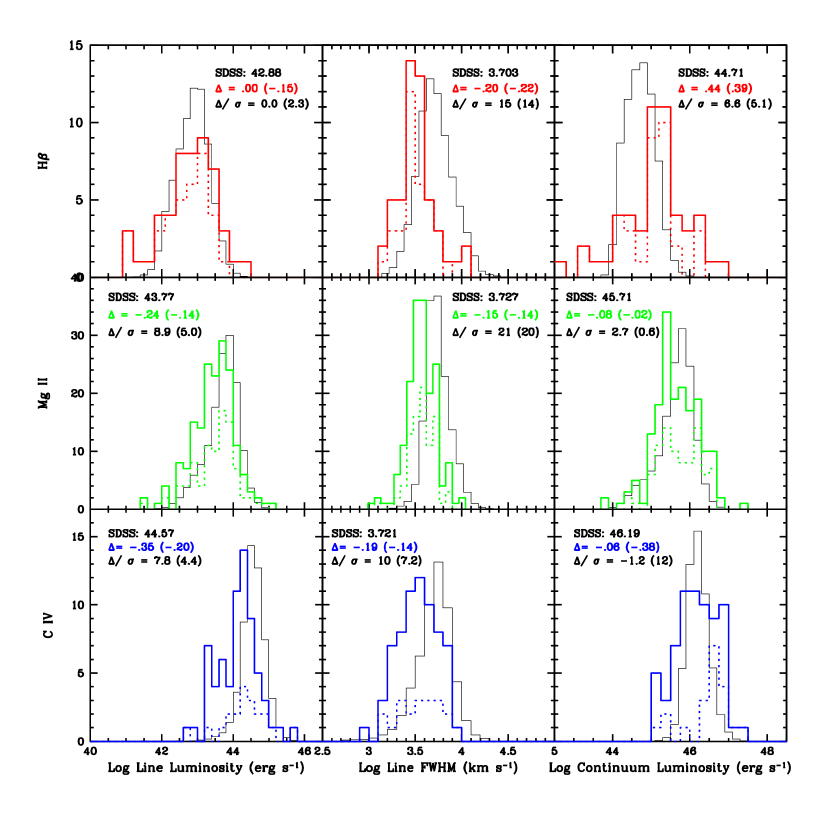
Figure 2.— Line and continuum properties of our 1LAC sample (thick colored lines) compared to the SDSS clean sample (Shen et al., 2011) (thin black lines). To match the flux limit of the clean sample, we additionally plot the subset of Fermi objects with magnitude $<19.1$ (dotted lines). For each species and parameter, the plots are labeled with the SDSS mean value and the offset $\Delta$ and estimated statistical significance $\Delta/\sigma$ of the means of the Fermi FSRQ, as measured in log space. The corresponding properties for the flux-limited sub-sample are given in parentheses.

To place our Fermi sample in the context of the broader QSO population, we compare our measurements to those of the largely ($>90\%$) radio quiet SDSS DR7 quasar sample (Shen et al., 2011). We find significant offsets in the mean values of the continuum luminosities, line luminosities, and line FWHMs of the two classes as plotted in Figure 2. Since our sample extends fainter than the SDSS QSOs, we also plot the distributions for a magnitude cut $i<19.1$ sample (Schneider et al., 2010).

To quantify these differences, we compute the medians, as well as the semi interquartile range (SIQR) for each distribution. We can use these values to estimate statistical errors on the median as $\sigma=SIQR/\sqrt{n}$, where $n$ is the number of points in the sample. In Figure 2, we report both the median offset, $\Delta$, and its estimated significance, $\Delta/\sigma$, for each parameter. The corresponding medians and errors for the magnitude-cut sample are given in parentheses.

Several distributions show large offsets from the SDSS population. Our C IV and Mg II lines are significantly less luminous than those of the SDSS QSOs. Comparing the values for the flux-cut sample, we see that a significant difference persists. We conclude that we are sampling a population with intrinsically weaker lines or that fainter, weaker-lines objects are lifted into our samples by the addition of extra non-thermal continuum flux. It seems that the local continua around Mg II and C IV are similar for our objects; we do notice that our H$\beta$ continua seem substantially brighter than those of the QSO population. We suspect that a lower redshift distribution, and larger host-light contribution (see below) may explain this effect.

For all species (and for the sub-sample) we find that our measured lines are significantly narrower than those the SDSS average. We attribute this to preferential alignment, further discussed in §6.

4. Excess Continuum

We expect our radio-$\gamma$ selected population to have significant continuum contribution from non-thermal jet emission. At low redshift, there may also be additional galaxy light, especially around the H$\beta$ line, to the red of the Balmer break.

4.1. Estimated Continua from Lines

In order to characterize the non-thermal emission in our spectra, we estimate a predicted continuum luminosity from the emission line fluxes, scaling to a non-blazar sample. Shen et al. (2011) reports line and continuum luminosities for the DR7 quasars. These are highly correlated (rxy = 0.85, 0.91, and 0.68 for H$\beta$, Mg II, and C IV respectively), and they fit continuum luminosities to line luminosities for Mg II and C IV, finding

$$\log L_{3000}=1.016\pm 0.003\cdot\log L_{\textrm{{Mg~{}II}}}+1.22\pm 0.11$$ (2)

$$\log L_{1350}=0.863\pm 0.009\cdot\log L_{\textrm{{C~{}IV}}}+7.66\pm 0.41$$ (3)

We extend this treatment by fitting the SDSS QSO results for the H$\beta$ line:

$$\log L_{5100}=0.802\pm 0.049\cdot\log L_{\textrm{H}\beta}+1.574\pm 0.060$$ (4)

Since the line flux continuum predictions are calibrated to a non-blazar sample, they should be independent of the non-thermal jet activity. Of course for both samples, at low redshift, there may still be galaxy light contaminating the H$\beta$ region, increasing the scatter. We compare the predicted to observed continuum levels for our Fermi FSRQ, finding that the lines predict (on average) $44\%$, $40\%$, and $32\%$ of observed continuum luminosities for H$\beta$, Mg II, and C IV respectively. We attribute the excess to non-thermal ‘jet’ emission.

It is of interest to inspect the non-thermal dominance ($NTD\equiv L_{obs}/L_{pred}$) for individual objects in our sample. While most objects have $NTD\sim 1$ (i.e. mostly thermal continua), for 57 blazars we have $NTD>2$ and 18 spectra show $NTD>10$ based on measurements of at least one line. We find significant correlation in same-object $NTD$ measured from the three species (rxy = 0.51 for Mg II and C IV; rxy=0.73 for H$\beta$ and Mg II) H$\beta$ generally measures larger $NTD$, which we attribute to contaminating galaxy light. Thus for $10\%$ of our sample, the spectra are BL Lac-like and analysis of the optical properties must account for this dominant non-thermal emission.

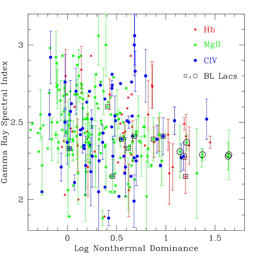
Figure 3.— The non-thermal dominance is the ratio of the measured to the predicted continuum emission near each of the lines. The H$\beta$ sample may be contaminated by galaxy luminosity as well. BL Lacs in the primary spectrum are circles. Squares indicate BL Lac designations from a previous spectrum. Large non-thermal dominance is weakly correlated to low spectral indices in Fermi observations. We thin error bars for $NTD<0.8$ for readability.

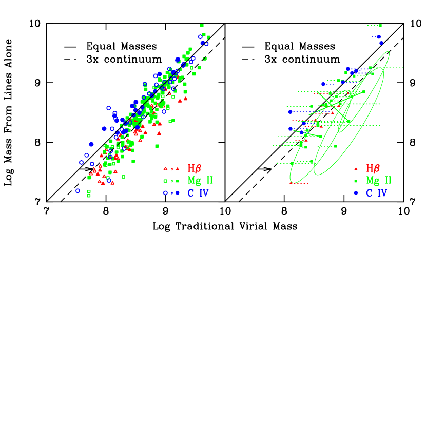
Figure 4.— On the left, masses from the lines are plotted against traditional virial masses for Fermi FSRQ. Most objects lie to the right of the 1:1 (solid) line, indicating larger traditional (continuum) masses. The dashed line shows the effect of a $3\times$ NTD. Closed symbols indicate objects with error $<0.4$ dex in both masses. In the right panel, objects with multiple observations are plotted. For the three objects with significant ($>2\sigma$) mass offset, we connect the two masses with a solid line, and plot the error ellipse around the primary observation. For others, we measure the continuum luminosity in both spectra, and mark the mass offset from continuum change by a dotted line.

4.2. Non-thermal Continuum Pollution

In Figure 3, we report on the $NTD$ of our sample. An optically selected population, such as that of Shen et al. (2011), peaks at $\log NTD=0$, the line-predicted thermal flux is comparable to the measured flux. Unsurprisingly the Fermi blazars extend to much larger $NTD$ levels. This plays an important role in continuum-calibrated estimates of hole mass in §5.

We further find a weak, but interesting correlation between NTD and Fermi $\gamma$-ray spectral index. The Fermi FSRQ population has $<\gamma>=2.44$, whereas the BL Lac population has $<\gamma>=2.04$. Thus the $\gamma$-ray hardness is a good predictor of the continuum strength in the broad band SED. Indeed, we find that the objects in our sample with the largest NTD show relatively hard Fermi spectra. It will be of interest to trace this trend deeper into the BL Lac population, although NTD estimates will be more difficult for this sample. Note that while actual BL Lacs (circles), unsurprisingly, are mostly in the high NTD regime, a number of nominal FSRQ are found in this region, as well.

5. The Central Engine

5.1. Traditional Virial Mass Estimates

As in Shen et al. (2011), we estimate traditional virial black hole masses from a relation of the form:

$$\log\left(\frac{M_{BH}}{M_{\odot}}\right)=a+b\log\left(\lambda L_{\lambda}\right)+2\log\left(\textrm{FWHM}\right)$$ (5)

where $a$ and $b$ are calibrated from reverberation mapping for each line species (McLure & Dunlop, 2004). The broad line FWHM, in km s^-1, and the continuum luminosity $\lambda L_{\lambda}$, in units of $10^{44}$ erg s^-1, are measured as described in §3.4, §3.5, and §3.6. Values of $a$ and $b$ are tabulated in Table 2 from Vestergaard & Peterson (2006) (hereafter VP06) for H $\beta$ and C IV and Vestergaard & Osmer (2009) (hereafter, VO09) for Mg II. A scatter of $\sim 0.4$ dex has been inferred for virial masses in optically selected samples (Shen et al., 2011).

For our Fermi sample we estimate mass from H $\beta$ for 50 objects, from Mg II for 176 objects, and from C IV for 68 objects. For 39 and 50 objects respectively, we measure mass from both H $\beta$ and Mg II, and from Mg II and C IV. Masses are reported in Table 3 and Table 4.

We urge caution in a naive interpretation of these masses, as applied to blazers. Due to the significant $NTD$ of our sample, we expect continuum luminosity to not scale as in the reverberation mapping sample, as discussed below in §5.2. Further, preferential alignment and a non-spherical BLR yields systematically narrower lines, as discussed in §6.

5.2. Mass Estimates from Lines Alone

Table 2Coefficients for Black Hole Mass Estimates

Source	H $\beta$		Mg II		C IV		Reference
	a	b	a	b	a	b
Mass from Continuum	0.672	0.61	0.505	0.62	0.660	0.53	MD04 (H$\beta$,C IV), VO09 (Mg II)
Mass from Lines	$1.63\pm.04$	$0.49\pm.03$	$1.70\pm.07$	$.63\pm.00$	$1.52\pm.22$	$.46\pm.01$	this work (H$\beta$), Shen et al. (2011) (Mg II, C IV)

Note. — Coefficients for the virial fitting relation in Equation 5. Coefficients derived from this work, McLure & Dunlop (2004, MD04), Vestergaard & Osmer (2009, VO09), and Shen et al. (2011)

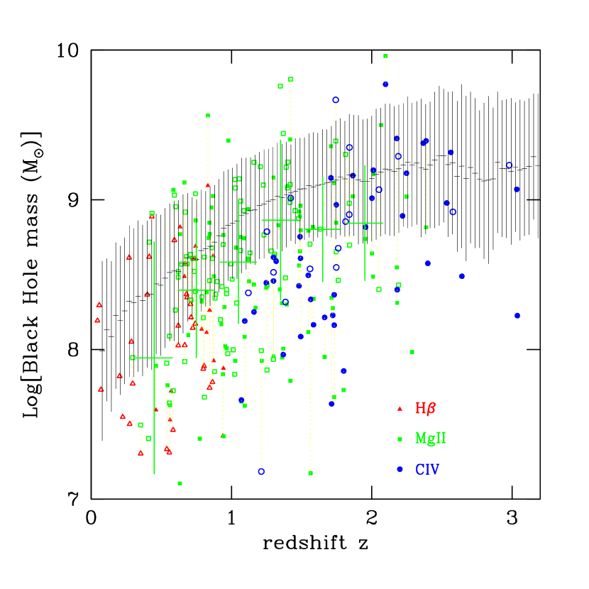
Figure 5.— Blazar black hole (line) masses as a function of redshift. Masses are over-plotted on the Sloan average quasar masses. Objects with $i<19.1$ are plotted as open points. Large green crosses show the average MgII-estimated mass and range for our magnitude-cut Fermi blazar sample in six redshift bins.

Bearing in mind the substantial NTD of much of our Fermi sample, we wish to make mass estimates from the line luminosity and line kinematic width alone. Greene & Ho (2005) and Kong et al. (2006) calibrate such estimators from reverberation mapping samples. Shen et al. (2011) calibrates estimators for Mg II and C IV from the SDSS sample. We have augmented this, using the SDSS mass estimators and developed our own coefficients for H$\beta$ with values consistent with the predicted continuum luminosity and mass estimates of §5.1. The coefficients for these estimators are listed in Table 2 for a formula of the form of Equation 5, replacing $\lambda L_{\lambda}$ with line luminosity in units of $10^{44}$ erg s^-1.

In Figure 4 we compare the line-estimated masses for our radio-$\gamma$ selected sample with estimates from the traditional continuum virial mass equations. We find the line masses are smaller than the traditional virial masses by 0.14 dex on average. This is a small, but significant effect. More interesting is the comparison for different species and different epochs. For example the nearby, low mass, low luminosity H$\beta$ mass sample shows a larger average line-mass decrease than the powerful C IV FSRQ. We attribute this primarily to host light pollution in the former and thermal disk domination in the latter.

For those objects where we have multiple epochs of observation (see §3.1 for details), we calculate the mass in both spectra. Due the statistical uncertainty in measuring the line kinematic width, and the large role that plays in mass calculations, in all but three cases, the measurement in the multiple spectra are not significantly different from that in the primary spectrum. In the right panel of Figure 4, we also plot estimated mass changes from continuum luminosity fluctuations in spectra too poorly measured to estimate line properties. The general trend is for variations to extend above the line-determined values, which show smaller fluctuation (i.e. continuum variations dominate and bias mass estimates, as expected).

5.3. Comparison to Optically Selected Quasars

Using the less biased masses derived using line strengths, we compare in Figure 5 our radio-$\gamma$ sample to the optically selected SDSS QSO (Shen et al., 2011). Interestingly, the mean mass varies with redshift in parallel to the QSO sample, but lower. For the full Fermi sample the offset is 0.44 dex. For the magnitude-cut sub-sample (directly comparable to the SDSS QSO), the offset is 0.34 dex.

The origin of this offset is unclear. Certainly the NTD of our sample causes some intrinsically fainter, less massive blazars to be boosted into our flux cut sample. Further, our Fermi objects sample a preferred orientation (see §6). Another possibility is that these sources are on average in a more active accretion state than the typical QSO (see §5.4). We also allow that the brighter blazars with with historical spectra in the literature may have systematically larger hole masses, decreasing the magnitude of this offset.

5.4. Eddington Ratio

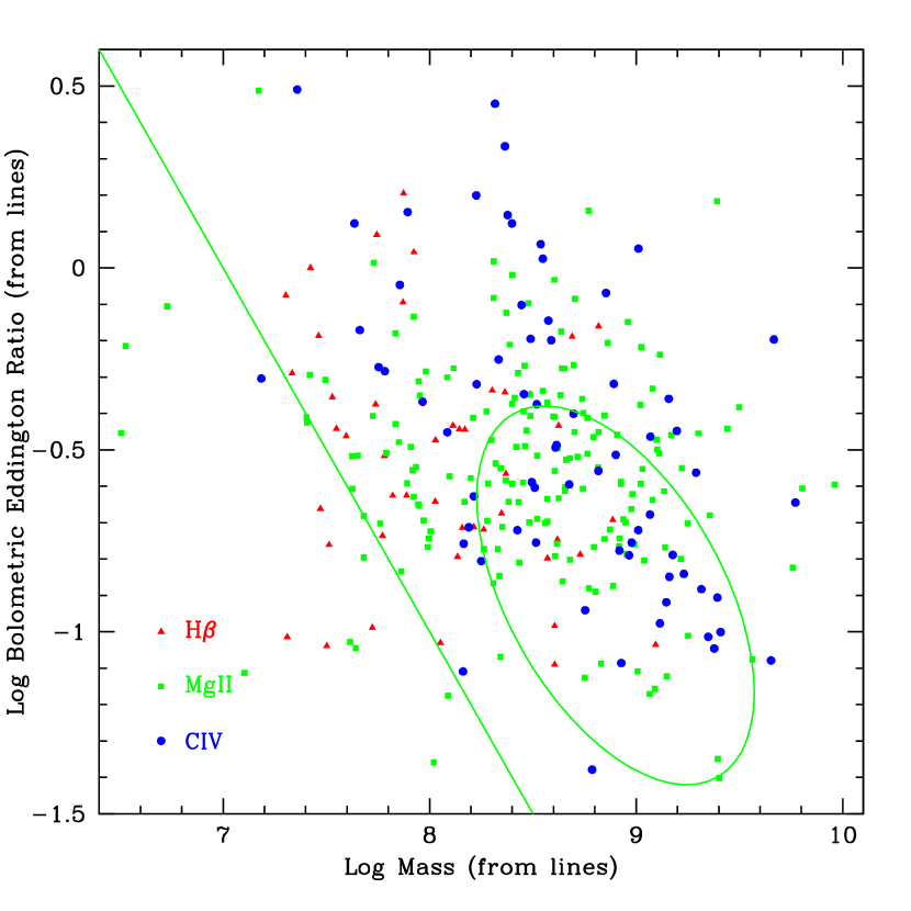
Figure 6.— The Eddington ratio plotted against black hole mass. The green ellipse shows the centroid and approximate 1$\sigma$ range for values determined from Mg II lines for the SDSS QSO sample. The green line shows the approximate flux limit for our sample.

Following the unified model (Urry & Padovani, 1995), we expect the quasi-isotropic thermal emissions of blazars to be similar to those in the underlying QSO population.

To probe this, we measure the disc luminosity in Eddington units, $L_{Edd}$, using line measurements alone. We first use the line fluxes to estimate local continuum luminosities, as above, then convert these to bolometric fluxes using factors from Richards et al. (2006) ($L_{bol}/L_{5100}=9.26$, $L_{bol}/L_{3000}=5.15$, $L_{bol}/L_{1350}=3.81$). This provides a bolometric thermal (= accretion power) luminosity, independent of any non-thermal contribution. This luminosity may be compared with the line-estimated hole masses to derive the Eddington ratio $L_{bol}/L_{Edd}$ for the population. Figure 6 displays this ratio against line-determined hole mass. Our sample has a systematically higher Eddington ratio and lower mass than the optically selected SDSS quasars. The radio-$\gamma$ selection probes an intrinsically more active population than an optically selected sample, both in flux limited samples.

Ghisellini et al. (2011) has proposed that FSRQ are more active accretors than BL Lacs. While our high Eddington ratios for this FSRQ support this picture, we do not find any inverse correlation between Eddington ratio and non-thermal dominance as might be expected if high values indicate a transition to a BL Lac-type state.

6. Orientation of the BLR

The virial black hole mass estimates require that the broad line region (BLR) has an isotropic velocity distribution (Salviander et al., 2007). In practice, there is a lack of consensus as to the shape of the BLR (McLure & Dunlop, 2004). With a more disc-like BLR, objects observed perpendicular to the disc will have lower kinematic FWHMs, and thus, lower inferred BH masses. Following Decarli et al. (2011), we can interpret the FWHM offset of §3.9 as a geometric effect and estimate the $f$-value, as a measure of the shape of the broad line region.

If we assume that the underlying broad line shape distribution is the same as that of the SDSS QSOs, and use our $i<19.1$ flux-cut sample, we find that our Mg II and C IV lines are 0.14 dex narrower. Recalling that our line widths seem to be systematically slightly lower than the SDSS line estimates by 0.04 dex, the true offset may be as high as 0.18 dex.

We assume we are probing a population with the same mass distribution as SDSS. Then, for a 0.14 dex offset our f-value is 1.38 $f_{\textrm{SDSS}}$, which is inconsistent with both a spherical BLR and a geometrically thin disk. In fact $f$ can be related to the typical disk thickness ratio H/R:

$$<f>=\left<0.5\left[\left(\frac{H}{R}\right)^{2}+\sin^{2}\theta\right]^{-1/2}\right>$$ (6)

where the average is taken over the observer inclination angle $\theta$. Since there is good evidence that the Fermi FSRQs are highly aligned (within 5^∘; Ajello et al, submitted to ApJ) by assuming that the SDSS QSO are viewed uniformly (in $\sin\theta$) away from the obscuring equatorial torus (at $\theta>60^{\circ}$), we obtain an estimate for $H/R\sim 0.4$. Since the function is very flat at low $\theta$, the result is insensitive to the precise degree of Fermi FSRQs alignment. In fact the required axis ratio only increases to 0.44 if the Fermi FSRQ are aligned within $2^{\circ}$. The decreased line width, and hence the decreased inferred hole mass are fully consistent with the preferred alignment of these blazars as expected in the Standard Model. Thus while we do not exclude underlying masses differences, our measurements are best explained by similar optically selected and radio-$\gamma$ selected black hole mass distributions, but with viewing angles strongly aligned to the disk (and jet) axis for the latter. As noted in §5.4, we do however find that the FSRQ show a higher Eddington ratio than the typical QSO, so some difference in accretion activity is indicated.

7. Comparison with Radio Activity

Since the Fermi FSRQ associations are largely selected from a sample of radio bright, flat-spectrum sources, it may be useful to compare the optical spectroscopic properties with radio measurements indicating strong non-thermal activity. One good measure of this activity is the radio variability. Much of the Dec $>$ -20 blazar sample has been monitored at 15 GHz at OVRO since before the launch of Fermi. These data have been used to measure the intrinsic modulation index, a measure of the activity:

$$\overline{m}=\frac{\sigma_{0}}{S_{0}}$$ (7)

where $S_{0}$ and $\sigma_{0}$ are the intrinsic mean flux density and its standard deviation of the radio light curve, estimated from the data using a maximum-likelihood method (Richards et al., 2011). It has, for example, been found that this index is smaller for high redshift FSRQ than lower redshift BL Lacs.

We might, therefore, expect this modulation to correlate with either the black hole mass Figure 7 or the NTD Figure 8. The lowest intrinsic modulations do appear among the highest mass holes, but there does not seem to be any increase in modulation for FSRQ with the higher NTD. Thus jet variability does not seem directly correlated with black hole and broad-line properties. It is possible that more significant differences may be traced to the radio variability timescale, but this requires longer radio monitoring and a more complete analysis of the flaring activity.

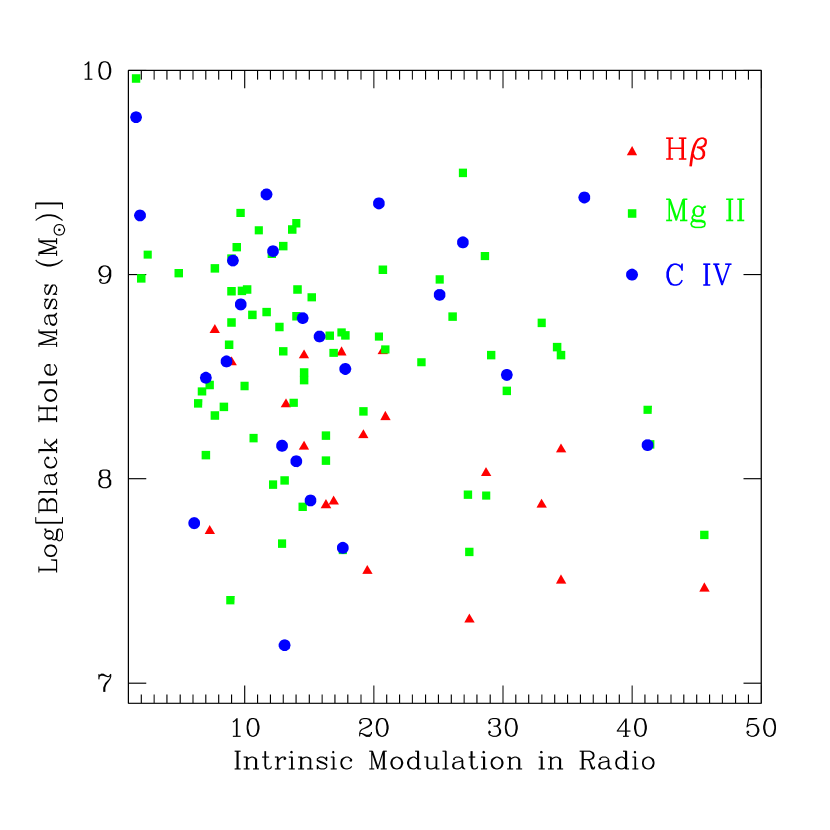
Figure 7.— The black hole mass is uncorrelated to the intrinsic modulation in radio.

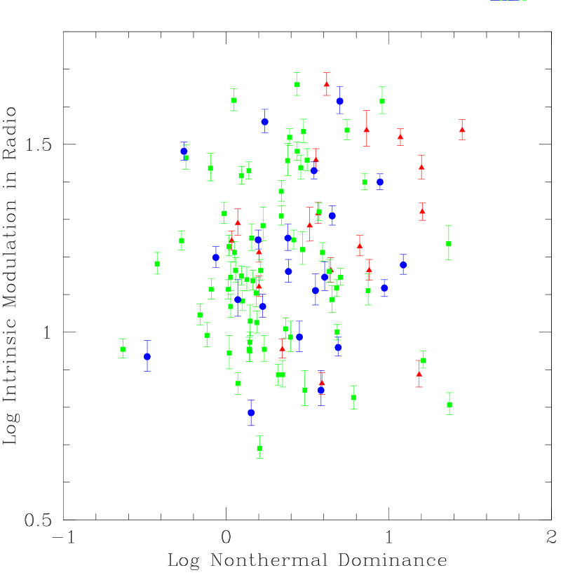
Figure 8.— The intrinsic modulation is uncorrelated to the non-thermal dominance of the optical spectrum.

8. Conclusions

We have used the optical spectral properties of our measured Fermi FSRQ sample to characterize the state of the central engine. We find that the optical continuum is significantly augmented by non-thermal (synchrotron) emission, presumably associated with the jet. In fact, such emission dominates the optical continuum for a third of our measured FSRQ. Unsurprisingly the degree of $NTD$ correlates with the $\gamma$-ray spectral index and the likelihood of BL Lac classification.

To avoid bias from the additional continuum, we have developed estimates of the black hole mass and the Eddington luminosity ratio which only use the line properties. These measurements show that the Fermi FSRQ are more active accretors than the bulk QSO population (at a given mass). We also find evidence for a significantly lower mean measured BH mass, even for a sample with a similar flux limit. Intriguingly, we find that the redshift evolution of the mass tracks that of the full QSO population. Thus, although non-thermal flux can pull less luminous, lower mass AGN into the sample, we speculate that the primary effect is due to the high expected degree of alignment for the FSRQ sample. If alignment is indeed the explanation, the data suggest a modest degree (H/R $\sim 0.4$) of flattening in the broad line region, and that we probe a similar mean mass population (and evolution) as the bulk QSO distribution.

While the present sample shows no strong correlation with the bulk radio variability, we expect that a broader look at the Fermi blazar sample, including comparison with the BL Lac properties and study of the BL Lac state-duty cycle and timescales for radio and optical modulation, will reveal additional correlations with the properties of the central black hole and its surrounding broad line region. This extension to the BL Lac portion of the sample is under way.

Table 3Line Properties for $z<1$ Broad Line 1LAC AGN

				H$\beta$				Mg II
Name	z	$F_{\nu,10^{14.7}}$	$\alpha$	$L_{5100}$	$L_{H\beta}$	FWHM	Mass	$L_{3000}$	$L_{\textrm{{Mg~{}II}}}$	FWHM	Mass	Telescope
	$10^{-28}$erg cm-2s-1Hz-1			erg s-1	erg s-1	kms-1	$\log\frac{M}{M_{\odot}}$	erg s-1	erg s-1	kms-1	$\log\frac{M}{M_{\odot}}$
J0004$-$4736	0.880	11.4$\pm$0.0	$-$0.99$\pm$0.08	…	…	…	…	45.339$\pm$0.011	42.896$\pm$0.151	2700$\pm$500	7.85$\pm$0.36	NTT
J0008+1450	0.045	73.8$\pm$0.1	$-$1.79$\pm$0.23	43.216$\pm$0.002	40.921$\pm$0.120	10800$\pm$2600	8.19$\pm$0.48	…	…	…	…	SDSS
J0017$-$0512	0.226	30.4$\pm$0.1	$-$0.46$\pm$0.36	44.353$\pm$0.004	42.388$\pm$0.107	2300$\pm$500	7.55$\pm$0.45	…	…	…	…	HET
J0024+0349	0.545	27.1$\pm$0.0	$-$1.88$\pm$0.08	…	…	…	…	45.110$\pm$0.001	42.585$\pm$0.057	3000$\pm$200	7.76$\pm$0.14	WMKO
J0043+3426	0.966	6.6$\pm$0.0	$-$1.24$\pm$0.03	…	…	…	…	45.201$\pm$0.006	42.807$\pm$0.072	3400$\pm$300	8.01$\pm$0.16	WMKO
J0050$-$0452	0.922	7.7$\pm$0.1	$-$0.92$\pm$0.19	…	…	…	…	45.198$\pm$0.013	43.140$\pm$0.141	3300$\pm$600	8.20$\pm$0.34	HET
J0102+4214	0.874	30.1$\pm$0.1	$-$1.63$\pm$0.86	46.001$\pm$0.004	43.460$\pm$0.038	1900$\pm$200	7.92$\pm$0.16	45.409$\pm$0.007	43.593$\pm$0.072	3300$\pm$300	8.49$\pm$0.17	WMKO
J0102+5824	0.644	167.0$\pm$0.3	$-$1.25$\pm$0.36	…	…	…	…	46.093$\pm$0.076	43.449$\pm$0.256	4100$\pm$1200	8.57$\pm$0.61	HET
J0112+2244	0.265	18.6$\pm$0.2	$-$2.71$\pm$0.79	…	…	…	…	…	…	…	…	HET
J0113+1324	0.685	15.2$\pm$0.0	$-$0.01$\pm$0.26	45.063$\pm$0.006	43.094$\pm$0.062	3800$\pm$500	8.35$\pm$0.25	45.263$\pm$0.006	43.389$\pm$0.082	4300$\pm$400	8.57$\pm$0.19	SDSS

Note. — Table 3 is published in its entirety in the electronic edition of this journal; A portion is shown here for guidance regarding its form and content.

Table 4Line Properties for $z>1$ Broad Line 1LAC AGN

				Mg II				C IV
Name	z	$F_{\nu,10^{14.7}}$	$\alpha$	$L_{5100}$	$L_{\textrm{{Mg~{}II}}}$	FWHM	Mass	$L_{3000}$	$L_{\textrm{{C~{}IV}}}$	FWHM	Mass	Telescope
	$10^{-28}$erg cm-2s-1Hz-1			erg s-1	erg s-1	kms-1	$\log\frac{M}{M_{\odot}}$	erg s-1	erg s-1	kms-1	$\log\frac{M}{M_{\odot}}$
J0011+0057	1.493	5.2$\pm$0.1	$-$0.51$\pm$0.05	45.486$\pm$0.021	43.541$\pm$0.081	4900$\pm$500	8.80$\pm$0.19	45.800$\pm$0.069	43.493$\pm$0.435	2500$\pm$1300	8.09$\pm$1.02	SDSS
J0015+1700	1.709	8.0$\pm$0.0	$-$2.75$\pm$0.38	46.070$\pm$0.004	44.178$\pm$0.043	5900$\pm$300	9.36$\pm$0.10	45.818$\pm$0.016	44.180$\pm$0.068	5900$\pm$500	9.15$\pm$0.17	WMKO
J0023+4456	2.023 :	1.3$\pm$0.1	$-$0.20$\pm$0.50	…	…	…	…	45.213$\pm$1.000	43.336$\pm$0.875	1900$\pm$2200	7.78$\pm$2.29	HET
J0042+2320	1.426	5.1$\pm$0.1	$-$1.40$\pm$0.08	45.533$\pm$0.017	43.412$\pm$0.137	6900$\pm$1100	9.01$\pm$0.32	…	…	…	…	HET
J0044$-$8422	1.032	9.7$\pm$0.0	$-$0.14$\pm$0.03	45.401$\pm$0.007	43.667$\pm$0.113	3900$\pm$500	8.68$\pm$0.26	…	…	…	…	VLT
J0048+2235	1.161	11.5$\pm$0.0	$-$1.34$\pm$0.18	45.639$\pm$0.002	43.143$\pm$0.049	4300$\pm$200	8.43$\pm$0.11	45.916$\pm$0.027	43.272$\pm$0.115	3400$\pm$500	8.25$\pm$0.28	WMKO
J0058+3311	1.369	3.1$\pm$0.1	$-$2.49$\pm$0.37	45.331$\pm$0.003	42.805$\pm$0.054	3400$\pm$200	8.01$\pm$0.13	45.177$\pm$0.035	43.451$\pm$0.076	2200$\pm$200	7.97$\pm$0.19	WMKO
J0104$-$2416	1.747	8.8$\pm$0.0	$-$0.81$\pm$0.22	45.817$\pm$0.010	43.613$\pm$0.111	5000$\pm$600	8.85$\pm$0.26	45.989$\pm$0.025	44.121$\pm$0.292	4900$\pm$1700	8.97$\pm$0.69	NTT
J0157$-$4614	2.287	1.9$\pm$0.0	$-$1.07$\pm$0.33	45.632$\pm$0.030	43.216$\pm$0.171	2500$\pm$500	7.98$\pm$0.40	45.522$\pm$1.000	44.083$\pm$7.015	3000$\pm$24900	8.52$\pm$20.15	VLT
J0226+0937	2.605	16.9$\pm$0.0	$-$0.58$\pm$0.26	…	…	…	…	46.811$\pm$0.006	44.582$\pm$0.720	8500$\pm$7500	9.65$\pm$1.76	P200

Note. — Table 4 is published in its entirety in the electronic edition of this journal; A portion is shown here for guidance regarding its form and content.

References

- Abdo et al. (2010a) Abdo, A. A., et al. 2010a, ApJS, 188, 405
- Abdo et al. (2010b) —. 2010b, ApJ, 720, 912
- Abdo et al. (2010c) —. 2010c, ApJ, 715, 429
- Appenzeller et al. (1998) Appenzeller, I., et al. 1998, The Messenger, 94, 1
- Atwood et al. (2009) Atwood, W. B., et al. 2009, ApJ, 697, 1071
- Bohlin (2007) Bohlin, R. C. 2007, in Astronomical Society of the Pacific Conference Series, Vol. 364, The Future of Photometric, Spectrophotometric and Polarimetric Standardization, ed. C. Sterken, 315–
- Buzzoni et al. (1984) Buzzoni, B., et al. 1984, The Messenger, 38, 9
- Decarli et al. (2011) Decarli, R., Dotti, M., & Treves, A. 2011, MNRAS, 413, 39
- Dekker et al. (1986) Dekker, H., Delabre, B., & Dodorico, S. 1986, in Presented at the Society of Photo-Optical Instrumentation Engineers (SPIE) Conference, Vol. 627, Society of Photo-Optical Instrumentation Engineers (SPIE) Conference Series, ed. D. L. Crawford, 339–348
- Ghisellini et al. (2011) Ghisellini, G., Tavecchio, F., Foschini, L., & Ghirlanda, G. 2011, MNRAS, 414, 2674
- Greene & Ho (2005) Greene, J. E., & Ho, L. C. 2005, ApJ, 630, 122
- Healey et al. (2008) Healey, S. E., et al. 2008, ApJS, 175, 97
- Jones et al. (2001–) Jones, E., Oliphant, T., Peterson, P., et al. 2001–, SciPy: Open source scientific tools for Python
- Kong et al. (2006) Kong, M.-Z., Wu, X.-B., Wang, R., & Han, J.-L. 2006, cjaa, 6, 396
- Krisciunas et al. (1987) Krisciunas, K., et al. 1987, PASP, 99, 887
- Kurtz & Mink (1998) Kurtz, M. J., & Mink, D. J. 1998, PASP, 110, 934
- McLure & Dunlop (2004) McLure, R. J., & Dunlop, J. S. 2004, MNRAS, 352, 1390
- Oke (1990) Oke, J. B. 1990, AJ, 99, 1621
- Richards et al. (2006) Richards, G. T., et al. 2006, ApJS, 166, 470
- Richards et al. (2011) Richards, J. L., et al. 2011, ApJS, 194, 29
- Salviander et al. (2007) Salviander, S., Shields, G. A., Gebhardt, K., & Bonning, E. W. 2007, ApJ, 662, 131
- Schlegel et al. (1998) Schlegel, D. J., Finkbeiner, D. P., & Davis, M. 1998, ApJ, 500, 525
- Schneider et al. (2010) Schneider, D. P., et al. 2010, AJ, 139, 2360
- Shen et al. (2011) Shen, Y., et al. 2011, ApJS, 194, 45
- Szokoly et al. (2004) Szokoly, G. P., et al. 2004, ApJS, 155, 271
- Tody (1986) Tody, D. 1986, in Society of Photo-Optical Instrumentation Engineers (SPIE) Conference Series, Vol. 627, Society of Photo-Optical Instrumentation Engineers (SPIE) Conference Series, ed. D. L. Crawford, 733–
- Urry & Padovani (1995) Urry, C. M., & Padovani, P. 1995, PASP, 107, 803
- Valdes (1986) Valdes, F. 1986, in Presented at the Society of Photo-Optical Instrumentation Engineers (SPIE) Conference, Vol. 627, Society of Photo-Optical Instrumentation Engineers (SPIE) Conference Series, ed. D. L. Crawford, 749–756
- Valdes (1992) Valdes, F. 1992, in Astronomical Society of the Pacific Conference Series, Vol. 25, Astronomical Data Analysis Software and Systems I, ed. D. M. Worrall, C. Biemesderfer, & J. Barnes, 417–
- Vestergaard & Osmer (2009) Vestergaard, M., & Osmer, P. S. 2009, ApJ, 699, 800
- Vestergaard & Peterson (2006) Vestergaard, M., & Peterson, B. M. 2006, ApJ, 641, 689
- Vestergaard & Wilkes (2001) Vestergaard, M., & Wilkes, B. J. 2001, ApJS, 134, 1