Modeling the near-UV band of GK stars, Paper II: NLTE models

Abstract

We present a grid of atmospheric models and synthetic spectral energy distributions (SEDs) for late-type dwarfs and giants of solar and 1/3 solar metallicity with many opacity sources computed in self-consistent Non-Local Thermodynamic Equilibrium (NLTE), and compare them to the LTE grid of Short & Hauschildt (2010) (Paper I). We describe, for the first time, how the NLTE treatment affects the thermal equilibrium of the atmospheric structure ($T(\tau)$ relation) and the SED as a finely sampled function of $T_{\rm eff}$, $\log g$, and $[{{\rm A}\over{\rm H}}]$ among solar metallicity and mildly metal poor red giants. We compare the computed SEDs to the library of observed spectrophotometry described in Paper I across the entire visible band, and in the blue and red regions of the spectrum separately. We find that for the giants of both metallicities, the NLTE models yield best fit $T_{\rm eff}$ values that are  30 to 90 K lower than those provided by LTE models, while providing greater consistency between $\log g$ values, and, for Arcturus, $T_{\rm eff}$ values, fitted separately to the blue and red spectral regions. There is marginal evidence that NLTE models give more consistent best fit $T_{\rm eff}$ values between the red and blue bands for earlier spectral classes among the solar metallicity GK giants than they do for the later classes, but no model fits the blue band spectrum well for any class. For the two dwarf spectral classes that we are able to study, the effect of NLTE on derived parameters is less significant. We compare our derived $T_{\rm eff}$ values to several other spectroscopic and photometric $T_{\rm eff}$ calibrations for red giants, including one that is less model dependent based on the infrared flux method (IRFM). We find that the NLTE models provide slightly better agreement to the IRFM calibration among the warmer stars in our sample, while giving approximately the same level of agreement for the cooler stars.

1 Introduction

Previously, we have compared the quality of fit provided by atmospheric models, high resolution synthetic spectra, and spectral energy distributions (SEDs, $f_{\lambda}(\lambda)$) computed both in LTE, and with many opacity sources treated in self-consistent Non-LTE (NLTE), for the the Sun and the standard stars Procyon ($\alpha$ UMi) and Arcturus ($\alpha$ Boo) ((Short & Hauschildt, 2009), (Short & Hauschildt, 2005), (Short & Hauschildt, 2003)). We found that our LTE models tend to increasingly predict too much blue and near-UV band flux as $T_{\rm eff}$ decreases, and that the problem is exacerbated by non-LTE effects (mainly the non-LTE over-ionization of Fe I, as is well explained in the case of the Sun (see, for example, Rutten (1986))). However, their conclusions were weak because of the small number of stars covering a few haphazard points in stellar parameter space ($T_{\rm eff}/\log g/[{{\rm A}\over{\rm H}}]$). Short & Hauschildt (2010) (hereafter Paper I) took a first step toward making the investigation more comprehensive by comparing a large grid of LTE model SEDs spanning the cool side of the HR diagram to observed SEDs taken from the extensive uniformly re-calibrated spectrophotometric catalog of Burnashev (1985). They investigated LTE models and synthetic SEDs computed with two choices of input atomic lines list: a larger, lower quality “big” list, and a smaller, higher quality “small” list, and found that the models computed with the “small” line list provide greater internal self-consistency among different spectral bands, and closer agreement with the less model-dependent $T_{\rm eff}$ scale of Ramirez & Melendez (2005), but not to the interferometrically derived $T_{\rm eff}$ values of Baines et al. (2010). They also found that to within the limits of the observed spectrophotometry, there was no evidence of a systematic over-prediction of blue and near-UV band flux among GK giants in general, but they did confirm the over-prediction for Arcturus (their “K1.5III-0.5” sample).

Here we take the next step by carrying out a similar comparison for a large grid of models SEDs with many important extinction sources treated in self-consistent NLTE (see Short & Hauschildt (2003) for a description of these atmospheric models and spectra with H, He, and two or more of the lowest ionization stages of C, N, O, and most of the light metals and the Fe-group elements treated in self-consistent multi-species non-LTE statistical equilibrium.) Our goal is to map out the goodness of fit, and the magnitude of any systematic discrepancies between model and observed SEDs, as a function of the three stellar parameters, $T_{\rm eff}$, $\log g$, and $[{{\rm A}\over{\rm H}}]$, this time for NLTE models, and to compare the results to those of LTE modeling. We also compare our $T_{\rm eff}$ values inferred from SED fitting to less model-dependent $T_{\rm eff}$ calibrations. One important goal is to determine where in the upper right quadrant of the HR diagram NLTE effects become most important.

2 Observed $f_{\lambda}(\lambda)$ distributions

Burnashev (1985) presented a large catalog (henceforth B85) of observed SEDs taken with photo-electric instruments on 0.5m class telescopes at various observatories in the former USSR from the late 1960s to the mid 1980s, and uniformly photometrically re-calibrated to the “Chilean system”. Short & Hauschildt (2009) contains a more detailed description of the individual data sources included in this compilation. These data sets all generally cover the $\lambda$ range 3200 to 8000 Å  with a nominal sampling, $\Delta\lambda$, of 25 Å, and have a quoted “internal photometric accuracy” of $\approx 3.5\%$. A point worth repeating from Paper I is that to match the appearance of the synthetic to the observed spectra, we had to convolve the synthetic spectra with an instrumental broadening kernel corresponding to a resolution element, $\Delta\lambda$, of 75 A.

Paper I contains a description of our procedure for extracting quality-controlled samples of spectra from the B85 catalog and forming mean and $\pm 1\sigma$ deviation spectra for each spectral type at each $[{{\rm A}\over{\rm H}}]$ value. We note here for the first time that our procedure effectively yields a useful spectrophotometric library for solar metallicity GK stars. To briefly summarize, the procedure involves cross-referencing the B85 catalog with the 5^th Revised Edition of the Bright Star Catalog (Hoffleit & Warren, 1991), henceforth BSC5) to screen out stars flagged as exhibiting binarity, chemical peculiarity, or variability of any kind. The B85 catalog does not contain metallicity information, therefore, we then identified our B85 stars in the metallicity catalog of Cayrel et al. (2001). For many, but not all, of our stars, the Cayrel et al. (2001) contains multiple $[{{\rm A}\over{\rm H}}]$ values. For objects where these were approximately randomly distributed, we found the mean metallicity. For objects where these had a skewed distribution, we disregarded the deviant values (usually only one)), and found a modal metallicity. We only retained stars for which the mean (or modal) $[{{\rm A}\over{\rm H}}]$ value was within $\pm 0.1$ of either of our two nominal $[{{\rm A}\over{\rm H}}]$ values of interest (0.0 and -0.5).

Spectral and luminosity classes were finalized by cross-referencing B85 stars with The Revised Catalog of MK Spectra Types for the Cooler Stars (Keenan & Newsom, 2000), the paper of Keenan & Barnbaum (1999), The Perkins Catalog of Revised MK Types for the Cooler Stars Keenan & McNeil (1989), or Skiff (2010), in decreasing order of preference. We also formed mean $B-V$ values for our spectral types by cross-referencing B85 stars with the Catalog of Homogeneous Means in the UBV System (Mermilliod, 1991). (As a result, we found the BSC5 catalog to accurately reflect the primary sources for these stars, and could have relied largely on it alone for spectral types and colors.) All spectra were corrected for their heliocentric radial velocity, RV, using the values in BSC5. However, we expect the RV correction to have a very minor effect on the quality of spectral fitting at the low spectral resolution of the B85 data.

In keeping with our automated approach, we make no attempt to find values in the literature (of possibly variable quality) for the distance and radius of each star. Rather, all spectra have been interpolating to a common regular $\lambda$ grid, and then a “quasi-bolometric” normalization was applied by dividing them by the entire area under the spectrum from 3200 to 7500 Å. We note that this differs from the normalization used in Paper I, in which the spectra were forced to have the same flux in a narrow spectral region around 6750 Å. We suspect that the normalization used in Paper I may artificially enhance the quality of fit at the red end of the spectrum with respect to that at the blue end, and is overly reliant on the absence of any unexpected features around 6750 Å. For each spectral type and $[{{\rm A}\over{\rm H}}]$ value, we calculate mean and $\pm 1\sigma$ deviation spectra for the sample of corresponding individual spectra. Table 1 of Paper I shows how many stars of each spectral/class and $[{{\rm A}\over{\rm H}}]$ value, and the number of spectra per star, were finally retained from the B85 catalog, along with the identities of the stars. In Table 1 we present summary information showing the total number of observed spectra that were used to form the mean and $\pm 1\sigma$ deviation spectra in each spectral class/$[{{\rm A}\over{\rm H}}]$ sample. Any individual spectra that deviated by more than $\approx 1\sigma$ from the sample mean over a significant $\lambda$ range were rejected and the mean and deviation spectra were re-calculated. This resulted in a final set of 44 spectra of 33 stars, 30 of $[{{\rm A}\over{\rm H}}]=0.0$ and three of $[{{\rm A}\over{\rm H}}]=-0.5$. Fig. 3 shows the comparison of the sample mean and $\pm 1\sigma$ deviation spectra to the distribution of individual spectra for the illustrative case of the G8 III/$[{{\rm A}\over{\rm H}}]=0.0$ sample.

Arcturus.

We note that our K1.5 III sample of $[{{\rm A}\over{\rm H}}]=-0.5$ consists entirely of three measurements of the spectrum of Arcturus. Therefore, the evaluation of NLTE and LTE fits to this sample is directly comparable to the NLTE modeling of Arcturus of Short & Hauschildt (2003) and Short & Hauschildt (2009).

3 Model grid

3.1 Atmospheric structure calculations

The grid of LTE spherical atmospheric models and synthetic SEDs computed with PHOENIX V. 150303C, covering $\approx$ 600 parameter points, was described in detail in Paper I. The most pertinent point to reiterate here is that the grid has sampling intervals, $\Delta T_{\rm eff}$, of 125 K and $\Delta\log g$ of 0.5. The grid covers $\log g$ values from 3.0 to 1.5 at all $T_{\rm eff}$ values from 4000 to 5625 K, goes to down to 1.0 for all models of $T_{\rm eff}\leq 5000$ K, and includes values from 4.0 to 5.0 for $T_{\rm eff}\geq 5375$ K. All models are computed at $[{{\rm A}\over{\rm H}}]$ values of 0.0 and -0.5. The radii of these spherical models were determined by holding the mass fixed at $1M_{\rm Sun}$, and the justification is described in Paper I and more extensively in the careful investigation of PHOENIX LTE models of red giants in the “NextGen” grid of Hauschildt et al. (1999). The value adopted for the micro-turbulent velocity dispersion, $\xi_{\rm T}$, increases from 1 to 4 km s^-1 as $\log g$ decreases. Based on numerical experiments with $\xi_{\rm T}$ values of 2 and 4 km s^-1 at $T_{\rm eff}=4000$ K, $\log g=1.0$, and $[{{\rm A}\over{\rm H}}]=0.0$, we find that the value has little discernible impact on the synthetic SEDs once they are convolved to match a spectral resolution element, $\Delta\lambda$, of 75 A. The atmospheres of GK stars become convective below a continuum optical depth of unity. PHOENIX employs the Böehm-Vitense mixing-length theory (MLT) of convection, and we adopted a mixing length parameter for the treatment of convective flux transport of one pressure scale height. Given the scope of the model grid required for this initial investigation, we have decided to restrict ourselves to scaled solar $[{{\rm A}\over{\rm H}}]$ distributions, with the solar abundance distribution of Grevesse et al. (1992). The considerations leading to this choice were discussed in Paper I, but are worth reiterating here given the recent discussion surrounding solar abundances (see, for example, Asplund et al. (2004)). There has been some tension between 3D NLTE spectroscopic abundances and helioseismological abundances that makes it difficult to clarify which abundances to prefer. We plan to extend our investigation in the future by exploring the effects of both alternate solar abundances, and non-solar abundances for metal-poor stars.

We note again here that our models are in hydrostatic and radiative/convective equilibrium, and are static and horizontally homogeneous. Therefore, they cannot account for the effects of chromospheric heating, nor for star spots, active regions, granulation, or other horizontal inhomogeneities.

3.1.1 NLTE

Short & Hauschildt (2005) contains a description of the method and scope of the NLTE statistical equilibrium (SE) treatment in PHOENIX and the sources of critical atomic data, and we only re-iterate the most pertinent aspects here. If necessary, PHOENIX can include at least the lowest two stages of 24 elements, including the lowest six ionization stages of the 20 most important elements, including Fe and three other Fe -group elements, in NLTE SE. This includes the inclusion of thousands of lines of Fe I and II in NLTE. Something that we have not described in previous papers is that we construct our atomic models using an automatic procedure that constructs the models from energy-level and atomic line data in the line lists of Kurucz (1992). The only input is the energy cut-off for the highest lying levels to be included in the atomic model. This has the very important advantage that the atomic data for the NLTE models is bound to be consistent with that of the LTE models. The supplementary data for radiative bound-free ($b-f$) and collisional cross-sections that are needed are described in Short & Hauschildt (2005).

For the species treated in NLTE, only levels connected by transitions of $\log gf$ value greater than -3 (designated primary transitions) are included directly in the SE rate equations. All other transitions of that species (designated secondary transitions) are calculated with occupation numbers set equal to the Boltzmann distribution value with excitation temperature equal to the local kinetic temperature, multiplied by the ground state NLTE departure co-efficient for the next higher ionization stage. We have only included in our NLTE treatment here those ionization stages that are non-negligibly populated at some depth in the Sun’s atmosphere. As a result, we only include the first one or two ionization stages for most elements. We therefore err on the side of including more ionization stages than are necessary for the late G and K class stars being modeled presently.

It is worth re-emphasizing here that our method of solving the coupled SE and radiative transfer equations is such that the SE solution is self-consistent across all NLTE species. For example, if transitions from two or more NLTE species overlap in wavelength, the SE solutions of the species will be correspondingly coupled as a natural consequence of the method. This is significant for late-type stars in which the spectrum is notoriously over-blanketed in the blue and near UV bands. Short & Hauschildt (2003) and Short & Hauschildt (2005) have studied the effect of including or excluding various groups of transitions in the NLTE SE and have found that the SE of the Fe-group elements has a significantly greater effect on the model structure and SED that the that of the “light metals”. For this investigation, we make no attempt to individually ”hand-tune” the values of atomic parameters for particular transitions as one should for careful spectroscopic abundance determination. Here, we are interested in the differential effect on the atmospheric structure and overall SED of models as a result of many opacity sources being treated in NLTE as compared to LTE, and our hope is that errors in the many NLTE transitions being treated will on average approximately cancel each other out.

We note that in NLTE mode, PHOENIX is currently restricted to the smaller, higher quality (“small”) atomic line list discussed in Paper I. Therefore, the LTE models used in the comparisons here are those of “Series 2” from Paper I. This “small” atomic line list consists of a 1.4 Gbyte list adapted from lists available on Kurucz’ ftp site as of 2007, except for those species treated in NLTE, for which the line list transitions are suppressed. For NLTE species, only those bound-bound ($b-b$) transitions accounted for in the model atoms represented by the SE equations are accounted for. The molecular line list is an 11 Gbyte file that includes all molecular opacity sources that are important in the Sun, among many other molecular opacity courses. This list was developed for PHOENIX modeling of brown dwarfs (see, for example, Helling et al. (2008)) and is more that adequate to account for molecular opacity in our coolest K stars.

The physics of NLTE radiative equilibrium (RE) is complex in that any given $b-b$ (line) or $b-f$ (photo-ionization edge) transition may either heat or cool the atmosphere when treated in NLTE with respect to LTE, depending on how rapidly the monochromatic optical depth, $\tau_{\lambda}$, increases inward at the wavelength of the line or $b-f$ edge, whether the transition falls on the Wien or the Rayleigh-Jeans side of the peak of the Planck function for the star’s $T_{\rm eff}$ value, and whether the transition is a net heater or coolant in LTE with respect to the gray atmosphere. An understanding of why the NLTE $T(\tau)$ structure differs from that of LTE in the way that it does would require a careful analysis of the role of any number of $b-b$ and $b-f$ transitions throughout the spectrum in establishing the NLTE RE. Such an analysis is beyond the scope of the present work. Careful investigations of NTLE RE for the special case of the Sun have been carried out by Anderson (1989) and Vernazza, et al. (1981).

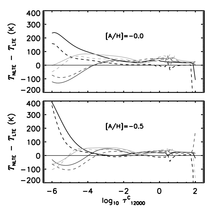
Figure 1: The difference in kinetic temperature of select NLTE and LTE models, $\Delta T_{\rm Kin}=T_{\rm NLTE}(\tau)-T_{\rm LTE}(\tau)$. The $x$-axis: Continuum optical depth at 12 000 Å, $\tau^{\rm C}_{\rm 12000}$. Results are shown for models of $T_{\rm eff}$ of 5500 K (black line), 4750 K (medium gray line) and 4000 K (light gray line) at $\log g$ values of 3.0 (solid line) and 1.0 (or 1.5 for the 5500 K model) (dotted line). Upper panel: $[{{\rm A}\over{\rm H}}]=0.0$; Lower panel: $[{{\rm A}\over{\rm H}}]=-0.5$.

Fig. 1 shows the difference in kinetic temperature of NLTE and LTE models, $\Delta T_{\rm Kin}=T_{\rm NLTE}(\tau)-T_{\rm LTE}(\tau)$, as a function of continuum optical depth at 12 000 Å, $\tau^{\rm C}_{\rm 12000}$, for select models spanning the grid and showing various representative behaviors throughout the grid, of $T_{\rm eff}$ equal to 4000, 4750, and 5500 K, $\log g$ equal to 3.0 and 1.0 (1.5 in the case of the 550 K model), and $[{{\rm A}\over{\rm H}}]$ values of 0.0 and -0.5. All models show some increase in $T_{\rm Kin}$, by as much as $\approx$ 200 K, for $\tau^{\rm C}_{\rm 12000}\leq-1$. For solar metallicity giants of $T_{\rm eff}\geq 5375$ K, this “NLTE heating” with respect to LTE continues to the top of the atmosphere. This NLTE RE effect has been previously found, and extensively discussed, in detailed NLTE investigations of the Sun’s atmosphere (Short & Hauschildt (2005), Anderson (1989)), and is caused almost entirely by the effect of NLTE on the Fe-group lines. The effect is enhanced by $\approx$ 100 K near the surface in the atmospheres of the mildly metal poor giants. However, for stars of $T_{\rm eff}<5375$ K, the effect of NLTE is to cool the atmosphere at higher layers ($\tau^{\rm C}_{\rm 12000}\leq-3$) by as much as $\approx$ 150 K. Photo-ionization ($b-f$) edges in the UV of Mg I ($\lambda 2514$), Al I ($\lambda 2076$), and Si I ($\lambda 1682$) are transitions that are strong in most of the models throughout our $T_{\rm eff}$ range, and occur in a spectral region where there is still enough flux that they might cool the atmosphere in NLTE with respect to LTE.

Note that $\Delta T_{\rm Kin}(\tau)$ behaves erratically at $\tau^{\rm C}>0$ because the $T_{\rm Kin}(\tau)$ structure steepens in the lower atmosphere where many radiative transitions become optically thick and the evaluation of $\Delta T_{\rm Kin}$ becomes numerically sensitive to this slope. However, this is also the $\tau^{\rm C}$ range in which convection rather than radiation increasingly determines the $T_{\rm Kin}(\tau)$ structure as $\tau^{\rm C}$ increases, and is not as useful for assessing the effect of NLTE on the RE $T_{\rm Kin}$ structure.

3.2 Synthetic spectra

For both LTE and NLTE models we computed self-consistent synthetic spectra in the $\lambda$ range 3000 to 8000 Å  with a spectral resolution ($R={\lambda\over\Delta\lambda}\approx 350\,000$) to ensure that spectral lines were adequately sampled. We note that the value of $\xi_{\rm T}$ was consistent between the spectrum synthesis and the input atmospheric models, as was all the stellar parameters. In the NLTE calculations, PHOENIX also automatically adds additional $\lambda$ points to adequately sample the spectral lines that correspond to $b-b$ atomic transitions that are being treated in NLTE. These were then degraded to match the low resolution measured $f_{\lambda}$ distributions of B85 by convolution with a Gaussian kernel of FWHM value equal to 75 Å. This is about three times the nominal sampling, $\Delta\lambda$, of 25 Å  claimed by B85, and we found that it provided the closest match to the appearance of the B85 spectra, as discussed in Paper I. We note that this convolution also automatically accounts approximately for macro-turbulence, which has been found to be around 5.0 km s^-1 for G and K II stars (Gray, 1982). We interpolate in $\log f_{\lambda}$ between adjacent synthetic SEDs to obtain a SED grid with an effective sampling, $\Delta T_{\rm eff}$, of 62.5 K. The accuracy of this interpolation was investigated in Paper I, and was found to be accurate to within 5% in linear flux among the coolest models where the variation in $f_{\lambda}$ with $T_{\rm eff}$ is greatest. This is about the same, or smaller, than the typical $\Delta T_{\rm eff}$ value between adjacent spectral subclasses for GK stars.

3.2.1 NLTE

Fig. 2 shows the relative difference of the NLTE and LTE synthetic SEDs, $100.\times(f_{\lambda,{\rm NLTE}}-f_{\lambda{\rm LTE}})/f_{\lambda{\rm LTE}}$, convolved to the effective resolution of the observed SEDs (75 Å) for the models of Fig. 1. Generally, the NLTE SEDs become increasingly brighter than the LTE SEDs as $\lambda$ decreases. This is a well-known effect that has been studied extensively in the Sun (see Rutten (1986), Anderson (1989)) and is caused by the NLTE over-ionization (really, LTE under-ionization!) of the minority Fe I stage. The NLTE effect on the Fe I/II ionization equilibrium reduces the extinction in the “forest” of Fe I lines that blanket the spectrum (the “iron curtain”) and allows more flux to escape. Because the lines are more densely concentrated per unit $\Delta\lambda$ as $\lambda$ decreases, the blue and near-UV bands are effected significantly more than the red band. This effect dominates any change in $f_{\lambda}$ that might be expected from the NLTE effect on the $T_{\rm Kin}$ structure that is seen in Fig. 1. As a result, we expect that fitting NLTE SEDs to observed SEDs would lead to a lower inferred $T_{\rm eff}$ value. For the coolest models in the grid ($T_{\rm eff}\leq 4125$ K), the NLTE spectra are also brighter in the regions of strong molecular bands, such as that of TiO around $\log\lambda=3.86$, as a result of the outer atmosphere being warmer in NLTE (see Fig. 1) and less favorable to molecule formation. As a result, we expect that fitting either the ratio of the blue- to red-band flux, or the strength of the molecular bands, would lead to a lower $T_{\rm eff}$ value when using NLTE models as compared to LTE models.

The synthetic SEDs were interpolated to the same regular $\lambda$ grid as that of the processed B85 spectra, and the same “quasi-bolometric” normalization was applied (see section 2). This normalization differs from the single-point normalization used in Paper I, and has the advantage of not biasing the fit of model to observed spectra to any particular wavelength.

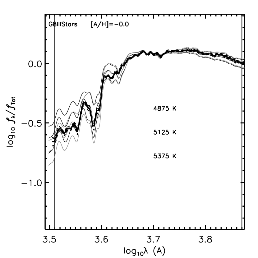
Figure 4: G8 III sample: Comparison of normalized observed sample average to select normalized synthetic $f_{\lambda}$ spectra of NLTE models. Thick solid line: sample average $f_{\lambda}$ spectrum, black dashed lines: $\pm 1~{}\sigma$ spectra. Thin solid gray-scale lines: select synthetic $f_{\lambda}$ spectra among those bracketing the model of best fit $T_{\rm eff}$ value at the smallest and largest $\log g$ values of the model grid; Dark gray: $\log g=3.0$, light gray: $\log g=1.0$.

As an illustrative example, Fig. 4 shows the comparison of the mean and $\pm 1\sigma$ spectra of the observed $f_{\lambda}$ distributions with a selection of NLTE synthetic $f_{\lambda}$ distributions for models bracketing the best fit $T{\rm eff}$ value at the smallest and largest $\log g$ values in the model grid for the G8 III/$[{{\rm A}\over{\rm H}}]=0.0$ sample. Fig. 5 shows the difference between the mean of the observed $f_{\lambda}$ distribution and a selection of NLTE synthetic distributions for models bracketing the best fit $T{\rm eff}$ value at the smallest and largest $\log g$ values in the model grid, relative to the observed mean distribution, $(f_{\lambda,{\rm Mean~{}Observed}}-f_{\lambda,{\rm Model}})/f_{\lambda,{\rm Mean~{}Observed}}$ for the same sample. We note that Paper I shows similar comparisons for the LTE synthetic spectra for a variety of samples.

4 Goodness of fit statistics

We compute on the interpolated $\lambda$ grid for each spectral class sample the root mean square relative deviation, $\sigma$, of the mean observed $f_{\lambda}$ distribution from the closest matching and bracketing convolved synthetic $f_{\lambda}$ distributions in the $\lambda$ range from 3200 to 7000 Å, according to

$$\sigma^{2}={1\over N}\sum_{i}^{N}((f_{\lambda,{\rm Obs}}-f_{\lambda,{\rm Mod}})/f_{\lambda,{\rm Obs}})^{2}$$ (1)

where $N$ is the number of $\lambda$ points in the $\lambda$ grid in the 3200 to 7000 Å  range. We also compute separate RMS values, $\sigma_{\rm Blue}$ and $\sigma_{\rm Red}$, for our nominal “blue” and “red” sub-ranges of 3200 to 4600 Å  and 4600 to 7000 Å, respectively. A comparison of the $\sigma_{\rm Blue}$ and $\sigma_{\rm Red}$ values indicates how well the synthetic spectra fit in the blue and near UV band given the quality of fit in the red band. A break-point of 4600 Å  was chosen on the basis of visual inspection of where the deviation of the synthetic from the observed spectrum starts to become rapidly larger as $\lambda$ decreases.

In Tables 2 and 3 we present the $\sigma$, $\sigma_{\rm Blue}$, and $\sigma_{\rm Red}$ values for the LTE and NLTE models, respectively, along with the best fit value of $T_{\rm eff}$ and $\log g$ for each star. The value of the model $[{{\rm A}\over{\rm H}}]$ is also tabulated, although, its value was specified a priori on the basis of the metallicity catalog of Cayrel et al. (2001) rather than fitted. As a check, we also computed $\sigma$ values for each sample with the $[{{\rm A}\over{\rm H}}]$ values of the models reversed; ie. we fitted models of $[{{\rm A}\over{\rm H}}]=0.0$ to samples formed from stars of catalog $[{{\rm A}\over{\rm H}}]$ equal to $\approx-0.5$ and vice versa. In most cases the $\sigma$ values of the metal-reversed fits were larger, and in a few cases were comparable to, those of the original fits. In no cases were they lower. We conclude that the $[{{\rm A}\over{\rm H}}]$ values of Cayrel et al. (2001) are generally reliable for GK stars to within $\pm\approx 0.25$. (For those stars within our spectral class range for which the catalog gives an uncertainty estimate, usually taken from the sources they are citing, their estimates range from 0.03 to 0.09. For Arcturus (K1.5 III), with 17 measurements, and HD62509 (K0 III) with seven measurements, the RMS deviations of $[{{\rm A}\over{\rm H}}]$ are 0.111 and 0.086, respectively.)

4.1 Trend with $T_{\rm eff}$

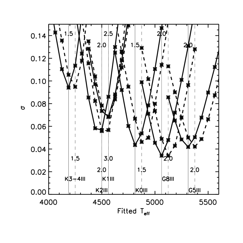
Figure 6: Giants of solar metallicity: Variation of $\sigma$ with model $T_{\rm eff}$. Solid line: NLTE models; dashed line: LTE models. Vertical lines: Best fit $T_{\rm eff}$ values. Best fit $\log g$ values are given for the LTE (lower row), and NLTE (upper row) models.

Fig. 6 shows the variation of $\sigma$ with model $T_{\rm eff}$ ($\sigma(T_{\rm eff})$ curves) for the giant stars of solar metallicity, for both LTE and NLTE models. The $\log g$ value of the best fit model for each spectral class is also indicated. The quality of the fit generally worsens with decreasing $T_{\rm eff}$, as is seen by the increase of $\sigma_{\rm Min}$ for later spectral class. As noted in Paper I, the density of spectral lines generally increases with increasing lateness. Therefore, this trend in the discrepancy between synthetic and observed SEDs could be explained by inadequacies in the input atomic data for bound-bound ($b-b$) transitions, or by inadequacies in the treatment of spectral line formation. Moreover, spectral features, especially those of molecules, are very sensitive to 3D effects Asplund (2000), and that also contributes to increasing discrepancies for the cooler models.

Interestingly, we note that the $\sigma_{\rm Min}$ values for the LTE and NLTE models differ negligibly from each other for all spectral classes. The adoption of NLTE does not improve the quality of fit provided by the best fit model. However, the value of the best fit NLTE $T_{\rm eff}$ is always one $\Delta T_{\rm eff}$ element (62.5 K) lower than the LTE value for giants of any spectral class. This was expected from the comparison of the LTE and NLTE $f_{\lambda}$ distributions in Section 3.2, and amounts to a uniform shift downward in the $T_{\rm eff}$ calibration of the GK III classification by $\approx$ 62.5 K. Unfortunately, because the shift is one $\Delta T_{\rm eff}$ element, we are barely resolving the shift numerically, and the actual shift could be anywhere in the range of about 30 to 95 K, and could vary with spectral class within this range. For all six spectral classes (Tables 2, 2), we find best fit $\log g$ values from NLTE modeling in the range of 1.5 to 2.5. For the LTE models the variation in best fit $\log g$ values is larger, with the K 1 III sample yielding a value of 3.0, which is near the upper limit for early K III stars. This may be taken a marginal evidence that the NLTE models provide more physically realistic parameters.

4.1.1 Red vs blue band

The quality of the best fit, as indicated by the value of $\sigma_{\rm Min}$, rapidly deteriorates for spectral classes later than K0 (Fig. 6). This is not unexpected; as $T_{\rm eff}$ decreases, the SED becomes increasingly line blanketed, particularly in the blue band, and the quality of the fit is increasingly dependent on the quality of atomic data and the treatment of line formation. Correspondingly, from Fig. 5 it can be seen that the difference spectra show increasing variability around the zero line as $\lambda$ decreases, in addition to any systematic trend away from the zero line. This can be seen more directly in Fig. 7, which shows the variation with $T_{\rm eff})$ of $\sigma$ for the blue ($\sigma_{\rm Blue}(T_{\rm eff})$) and red ($\sigma_{\rm Red}(T_{\rm eff})$ bands separately. For samples of spectral class K0 and warmer, the $\sigma{\rm Red},Min$ value is lower than the $\sigma_{\rm Blue},Min$ value by $\approx 0.05$ because the longer $\lambda$ range is less complicated by line blanketing. This discrepancy between $\sigma_{\rm Blue,Min}$, and $\sigma_{\rm Red,Min}$ increases rapidly for later spectral classes. We note that for all spectral classes, the -62.5 K $\Delta T_{\rm eff}$ offset between best fit NLTE and LTE models is also found separately in the blue and red bands.

For the G8 and K0 III $[{{\rm A}\over{\rm H}}]=0.0$ spectral classes (the special case G5 III is discussed separately in Section 4.1.2), the red and blue bands yield the same best fit value of $T_{\rm eff}$. This consistency across wave bands that have very different amounts of line blanketing provides some assurance of the the quality of the modeling, but does not distinguish the quality of the NLTE treatment from that of the LTE. For the K1 III $[{{\rm A}\over{\rm H}}]=0.0$ sample the best fit $T_{\rm eff}$ value found from the blue band is one $\Delta T_{\rm eff}$ element (62.5 K) cooler than that found from the red band. This may indicate that the NLTE treatment over-estimates the amount of NLTE blue-band $f_{\lambda}$ brightening (discussed is Section 3.2), thus leading to an artificially low $T_{\rm eff}$ value with respect to the less blanketed red band. This is consistent with the results of Short & Hauschildt (2009) for Arcturus (K1.5 III). However, for the K2 and K3-4 III $[{{\rm A}\over{\rm H}}]=0.0$ samples, the best fit $T_{\rm eff}$ value found from the blue band is 62.5 K hotter than that found from the red band, indicating that for the most heavily line blanketed giants considered here, the NLTE treatment under-estimates the amount of NLTE blue-band $f_{\lambda}$ brightening (discussed is Section 3.2), thus leading to an artificially high $T_{\rm eff}$ value with respect to the less blanketed red band.

For the metal-poor giant samples the situation is also confused: For the G8 III $[{{\rm A}\over{\rm H}}]=-0.5$ sample the $T_{\rm eff}$ value derived from the blue band is 62.5 K hotter than that from the red band, whereas it is 62.5 K cooler in the case of the K1.5 III $[{{\rm A}\over{\rm H}}]=-0.5$ sample (Arcturus). We note that for the case of Arcturus, for which the observed spectra presumably have the best quality, the use of NLTE models reduces the size of the $T_{\rm eff}$ discrepancy between blue and red bands from 125 to 62.5 K.

The lack of any clear trend between the sign of the blue- and red-band $T_{\rm eff}$ results and spectral class most likely is a reflection of the lack of good fit in the blue band provided by any model. Any signal in the value of the fitting statistic indicating how well any model fits at those wavelength windows where the fit is good is diluted by the “noise” from all the wavelength windows where all models, including the best fit one, are grossly discrepant with the observations.

4.1.2 G5 III sample

As noted in Paper I, the behavior of the variation of the $\sigma_{\rm Red}(T_{\rm eff})$ curve for the G5 III stars is peculiar and leads to a spurious result for the best fit value of $T_{\rm eff}$. From Fig. 7 of Paper I it can be seen that this is caused by a broad absorption feature exhibited by the observed SED with respect to the model SEDs ranging from a $\log\lambda$ value of 3.753 to 3.774 (5660 to 5940 Å). As a result, the value of $\sigma_{\rm Red}$ is increased significantly, even for models that provide a good match to the overall spectrum. Therefore, our best fit value of $T_{\rm eff}$ for the G5 III models is best determined from the blue band alone. This deficit of absorption in the synthetic SEDs with respect to the observed ones is consistently present in the individual observed spectra for the G5 III stars, spans 12 data points in the raw observed spectrum, and varies smoothly with wavelength over a range of  280 Å. We note that this discrepancy is either absent, or much less pronounced, in both the G4-5 V and G8 III stars, so appears to be localized in both $T_{\rm eff}$ and $\log g$. In Paper I we compared our three G5 III spectra from the B85 catalog with spectra for G4 and G6 III stars in the stellar spectrophotometric library of Jacoby et al. (1984) and concluded that this discrepancy is likely caused by a data acquisition or calibration error in the B85 data.

4.2 Trend with $[{{\rm A}\over{\rm H}}]$ and $\log g$

Figs. 8 and 9 show the $\sigma(T_{\rm eff})$ curves for the whole band fits for the G0 and G4-5 V ($[{{\rm A}\over{\rm H}}]=0.0$) samples, and the giant samples of $[{{\rm A}\over{\rm H}}]=-0.5$ (G8 and K1.5), respectively. Also shown are $\sigma(T_{\rm eff}$) curves for select giants of $[{{\rm A}\over{\rm H}}]=0.0$ for comparison. Because of the special problem of the red band in our G5 III sample (discussed in Section 4.1.2), we show the result of the G5 III fit in the blue band in Fig. 9. The best fit parameters for the whole band, and for the red and blue bands are also given in Tables 2 and 3.

For the metal poor giants (Fig. 8), the results are qualitatively similar to those for the solar metallicity giants: NLTE models give minimum $\sigma$ values that are effectively the same as those of LTE models at each spectral class, and the NLTE grid yields best fit $T_{\rm eff}$ values that are one $\Delta T_{\rm eff}$ element cooler that those of LTE grid. We note that at a given spectral class, the quality of fit ($\sigma_{\rm Min}$ value) is worse as $[{{\rm A}\over{\rm H}}]$ decreases, which may initially seem unexpected if the treatment of line blanketing is the greatest obstacle to achieving a good match. However, we note that $T_{\rm eff}$ is correlated with $[{{\rm A}\over{\rm H}}]$ at fixed spectral class (eg. both the G8III/-0.5 and K1.5III/-0.5 samples are 300 to 350 K cooler than the G8III/0.0 and K2III/0.0 samples, respectively) and so the real trend is likely to be the same correlation between $\sigma_{\rm Min}$ and $T_{\rm eff}$ that was seen for solar metallicity giants Fig. 6.

For the dwarfs (Fig. 9), the LTE and NLTE models yield the same best fit values of $T_{\rm eff}$. However, the $\sigma(T_{\rm eff})$ curves are flatter, and those of the NLTE models are skewed toward lower $T_{\rm eff}$ than those of the LTE models. For both dwarf spectral classes, $\sigma(T_{\rm eff}(\sigma_{\rm Min})-1\Delta T_{\rm eff})$ is approximately the same as $\sigma(T_{\rm eff}(\sigma_{\rm Min}))$. We infer that for class V stars, the NLTE reduction in the value of $T_{\rm eff}$ also exists, but that is it $\approx 0.5\Delta T_{\rm eff}$ (ie. $\approx$ 31 K).

4.3 Arcturus

From a comparison of Tables 2 and 3 for the Arcturus sample (K1.5 III, $[{{\rm A}\over{\rm H}}]=-0.5$) the $T_{\rm eff}$ value from the LTE blue band fit is 125 K lower than that from the red band, whereas with the NLTE modeling, it is only 62.5 K lower. That the NLTE grid yields $T_{\rm eff}$ values that are more consistent across wave bands provides some evidence that these models are more realistic. However, that there is still a discrepancy at all indicates that our NLTE models may be over-estimating the blue $f_{\lambda}$ level, and hence leading to an artificially low $T_{\rm eff}$ value, with respect to the red band. This is consistent with the results of Short & Hauschildt (2003) and Short & Hauschildt (2009), who also compared models to the observed $f_{\lambda}$ distribution of B85. Note that this is the opposite to what was found for the solar metallicity K2 III sample, so the effect may be metallicity dependent.

5 Comparison to other $T_{\rm eff}$ calibrations

In Paper I we compared our various LTE $T_{\rm eff}$ values to the less model dependent calibrations from the infrared flux method (IRFM) of Ramirez & Melendez (2005) (RM05), and from interferometric angular diameters of K giants determined with the CHARA array Baines et al. (2010) (B10), with a brief summary of these calibrations, a justification for these comparisons, and a discussion of how we interpolated or extracted appropriate $T_{\rm eff}$ values for comparison. We note that RM05 and B10 estimate their $T_{\rm eff}$ values to be accurate to $\pm 75$ K and 50 to 150 K (2 - 4%), respectively. Here we choose to compare our NLTE results to RM05 and B10 again, along with recently derived $T_{\rm eff}$ values for large samples of G and early K giants from three additional sources. Wang et al. (2011) derived $T_{\rm eff}$ values for 99 G-type giants by requiring the $[{{\rm Fe}\over{\rm H}}]$ values derived from Fe I lines in spectra acquired with the High Dispersion Spectrograph (HDS, $R=60\,000$) at the Subaru Telescope in the 4900 - 7600 Å  range to be independent of the excitation energy of the lower level ($\chi_{\rm l}$). $[{{\rm Fe}\over{\rm H}}]$ values are derived from the equivalent widths, $W_{\lambda}$, of Fe lines. They also independently re-derived $T_{\rm eff}$ from photometric $T_{\rm eff}$ relations of Alonso et al. (2001) and reddening laws in the literature combined with catalog values of a number of photometic indices. For the latter they estimate an uncertainty of $\pm\approx 100$ K from the $T_{\rm eff}-B-V$ relation. They note that the $T_{\rm eff}$ values from the Fe I lines are on average $44\pm 117$ K larger than those derived from photometric calibrations. Takeda, et al. (2008) used ATLAS9 atmospheric models to derive atmospheric parameters and $[{{\rm Fe}\over{\rm H}}]$ values from the $W_{\lambda}$ values of Fe I and II lines in the 5000 - 6200 Å  region of 322 bright ($V<6$) late-G giants with spectra ($R=67\,000$) obtained with the HIDES spectrograph at the 1.88 m telescope of the Okayama Astrophysical Observatory. They determine statistical uncertainties in their $T_{\rm eff}$ values of 10 - 30 K. Mishenina et al. (2006) used line depth ratios (from 70 to 100 ratios per star) to determine $T_{\rm eff}$ values for  200 late-G and early-K clump giants with spectra in the 4400 - 6800 Åregion ($R\approx 42\,000$) from the ELODIE echelle spectrograph at the 1.93 m telescope of the Haute-Provence Observatoire. They determine that the $1\sigma$ uncertainties are 5 to 25 K. They also determine $[{{\rm Fe}\over{\rm H}}]$ values from the $W_{\lambda}$ values of Fe I lines while requiring that all Fe I and II lines yield the same abundance to fix $\log g$ and $\xi_{\rm T}$. For the latter three studies, we extracted stars for which the derived $[{{\rm Fe}\over{\rm H}}]$ value was within 0.1 of either of the two $[{{\rm A}\over{\rm H}}]$ values of our model grid (0.0 and -0.5).

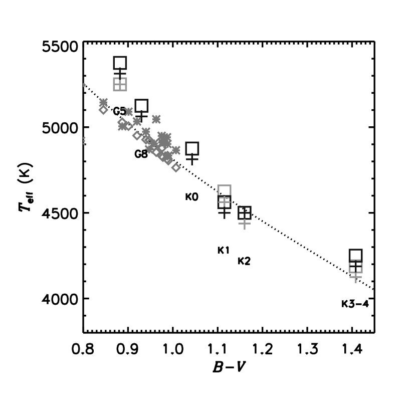
Figure 10: Solar metallicity giants: Comparison of our best fit $T_{\rm eff}$ values with various calibrations of $T_{\rm eff}$ as a function of $B-V$. Squares: LTE models; Crosses: NLTE models. Black symbols: Fit to the blue band; Gray symbols: fit to the red band. Note that for some cases the red and blue band symbols exactly overlap. Calibrations of RM05 (dotted line), Wang et al. (2011) photometric (diamonds), and Wang et al. (2011) spectroscopic (asterisks).

One point worth reiterating from Paper I is that the RM05 calibration is especially useful because it spans a wide range of values of $B-V$ and $[{{\rm A}\over{\rm H}}]$ at luminosity classes V and III. Therefore, we are able to compare all our results to RM05. We have extracted from the published tables of Wang et al. (2011), Takeda, et al. (2008), and Mishenina et al. (2006) samples of giants with $-0.1<[{{\rm A}\over{\rm H}}]<0.1$ and $-0.6<[{{\rm A}\over{\rm H}}]<-0.4$ for comparison to our results for our $[{{\rm A}\over{\rm H}}]=0.0$ and $-0.5$ samples, respectively. In Paper I, to facilitate the comparison, we computed mean and RMS ($\sigma$) $B-V$ values for each of our spectral class samples using colors for individual objects from the Catalog of Homogeneous Means in the UBV System (Mermilliod, 1991). We use the same mean colors for our samples here. In Table 4 and Figs. 10 through 12 we present a comparison of our $T_{\rm eff}$ values fitted to our blue and red spectral ranges, and those of the RM05 and B10 calibrations. We note from Fig. 10 that the photometrically derived $T_{\rm eff}$ values of Wang et al. (2011) agree very closely with the calibration of RM05. This is expected because Wang et al. (2011) and RM05 both make use of the photometric index versus $T_{\rm eff}$ relations of Alonso et al. (2001) (and papers in that series).

5.1 Solar metallicity giants

Our LTE models match the RM05 calibration to within the precision of the grid ($\rm 62.5$ K) for the latest spectral classes, and increasingly predict too large a $T_{\rm eff}$ value, by as much as $\approx 300$ K as $B-V$ decreases. This seems surprising given that the later-type stars have more complicated SEDs that are more difficult to model, as discussed above. This may reflect of a “conspiracy” of canceling errors at the latest spectral classes, and the result should be approached with caution. Again, we caution that the red band result for the G5 III sample is spurious for the reasons discussed above. Recently, Casagrande et al. (2010) have published a new IRFM $T_{\rm eff}$ scale (with I. Ramirez and J. Melendez as co-authors) for stars of $\log g>3.0$ and find that the scale is warmer by  85 K than that of RM05 for stars of $T_{\rm eff}\geq\approx 5000$ K while agreeing more closely with RM05 for cooler stars. This deviation from the RM05 scale results from a change in the absolute calibration of the photometry, therefore, it is expected to also apply to lower gravity stars. If it does, then our results may be in closer agreement with the IRFM calibration across the whole range of spectral classes studied here. Our LTE results are in similarly close agreement to the K giant $T_{\rm eff}$ calibration of B10. Because our NLTE $T_{\rm eff}$ scale is 62.5 K lower than the LTE scale, the NLTE models predict too low a $T_{\rm eff}$ value for the latest types, and a value that is closer to that of RM05, but still to large, for the earlier types. We note that the results of B10 are based on limb-darkening derived from 1D atmospheric models, and that Chiavassa et al. (2010) recently found that limb-darkening from 3D models leads to smaller derived radii and $T_{\rm eff}$ values that are correspondingly larger by as much as  20 K for stars of $T_{\rm eff}$ in the range 4600 to 5100 K (spectral classes K0 to G5) and $[{{\rm A}\over{\rm H}}]$ of -1, and by a smaller amount for stars of $[{{\rm A}\over{\rm H}}]$ of 0.0. It is intriguing that the sign of the 3D correction is one that would bring the B10 results into closer agreement with our NLTE $T_{\rm eff}$ values for the corresponding spectral classes.

We note that the $T_{\rm eff}$ values for individual stars derived by Wang et al. (2011) from the Fe I/II balance are also generally larger than RM05, and are in closer agreement with our values. Because our method is also essentially spectroscopic rather than photometric, this might seem to be evidence for spectroscopic $T_{\rm eff}$ determinations being generally 50-100 K larger than photometric determinations. However, the photometric $T_{\rm eff}$ scale is dependent upon the absolute calibration adopted, and we caution against drawing a conclusion on the basis of this work. The $T_{\rm eff}$ values for individual stars of Takeda, et al. (2008) and Mishenina et al. (2006) for G giants show a significant scatter and our $T_{\rm eff}$ values lie near the upper limit of their results. We have computed star-count weighted means of their $T_{\rm eff}$ values and also show them in Fig. 11. Our values for G giants are larger than this mean trend, as was found for our comparison to the RM05 calibration.

5.2 Solar metallicity dwarfs and metal poor giants

RM05 is the only calibration we have to compare our results to for class V stars. Our results for G dwarfs are better than those for for G giants, in that for both the G0 and G4-5 samples our blue band NLTE $T_{\rm eff}$ values are just slightly warmer than the RM05 calibration, by one $\Delta T_{\rm eff}$ element (62.5 K). For G stars, we infer that our NLTE modeling is increasingly accurate as $\log g$ increases. This may reflect that our 1D horizontally homogeneous static models become increasingly inaccurate as $\log g$ decreases.

Our LTE $T_{\rm eff}$ value for the K1.5 III sample of $[{{\rm A}\over{\rm H}}]=-0.5$ (consisting entirely of Arcturus spectra, recall) provides about the same quality of match to the RM05 calibration as that of our K1 and K2 III samples of $[{{\rm A}\over{\rm H}}]=0.0$. At the same time, our LTE $T_{\rm eff}$ value for the metal poor G8 III sample is much closer to the RM05 calibration than that of the solar metallicity G8 III sample. The NLTE blue band fit at G8 III/$[{{\rm A}\over{\rm H}}]=-0.5$ is very close RM05, whereas the NLTE results are cooler than RM05 by $\approx 150$ K at K1.5 III/$[{{\rm A}\over{\rm H}}]=-0.5$. We tentatively infer that our ability to reproduce the RM05 calibration with NLTE models for the earlier GK spectral classes improves with decreasing metallicity in this $[{{\rm A}\over{\rm H}}]$ range. This is not unexpected given the decreasing dependence on the realism of the line blanketing treatment as $[{{\rm A}\over{\rm H}}]$ decreases.

6 Conclusions

Our strongest conclusion is that the adoption of NLTE for many opacity sources shifts the spectrophotometrically determined $T_{\rm eff}$ scale for giants downward by an amount, $\Delta T_{\rm eff}$, in the range of about 30 to 90 K all across the mid-G to mid-K spectral class range, and across the $[{{\rm A}\over{\rm H}}]$ range from 0.0 to -0.5. This shift brings our spectrophotometrically derived $T_{\rm eff}$ scale for the solar metallicity G giants into closer agreement with the less model-dependent $T_{\rm eff}$ scale determined by the IRFM, although our $T_{\rm eff}$ values for these G giants are too large in any case. For the K giants, LTE and NLTE models provide about the same quality of match, and are closer to the less model-dependent IRFM $T_{\rm eff}$ values than is the case for the G giants. We find tentative evidence on the basis of two spectral classes in the G range that this NLTE downward shift in the $T_{\rm eff}$ scale becomes smaller as luminosity class increases from III to V.

Both NLTE and LTE model SEDs show a much greater variation about the observed SED in our more heavily line blanketed “blue” band ($\lambda<4600$ Å) than in the red band. This probably indicates that there are inadequacies in the accuracy and completeness of the atomic line list data and in the treatment of line formation. The latter inadequacy may in part be a result of our use of static 1D models. Nevertheless, we find somewhat surprising agreement in the best fit value of $T_{\rm eff}$ between the blue and red bands. There is marginal evidence that NLTE models seem to give more consistent results between the blue and red bands for the earlier spectral classes (G8-K0) of solar metallicity than for later classes. Moreover, there is marginal evidence that the derived $\log g$ values are more consistent between the red and blue bands from NLTE modelling than that of LTE.

Presumably, the highest quality observed SED in library is that for the K1.5III/$[{{\rm A}\over{\rm H}}]\approx-0.5$ sample, which consists of three independent measurements of the spectrum of the bright standard red giant Arcturus. We find that our NLTE grid provides greater consistency in derived $T_{\rm eff}$ value between our blue and red bands than does the LTE grid. However, we find that the blue band yields a $T_{\rm eff}$ value that is still lower than that of the red band (by nominally 62.5 K), indicating that NLTE models of red giants predict too much flux in the blue band with respect to the red band. This is a recurrence of a long-standing problem with the modeling of late-type stellar SEDs (see Short & Hauschildt (2009)), and may indicate an inadequacy in the atmospheric modeling of such stars. However, we do not find strong evidence of this blue band versus red band discrepancy among our many solar metallicity SED fits, and speculate that it may be a discrepancy that worsens with decreasing metallicity.

As a by-product of this investigation, we have produced a quality-controlled stellar library of observed mean and $\pm 1\sigma$ SEDs for solar metallicity giants that well sample the range from G8 to K4 III. We will make both the library of observed SEDS and the NLTE (and corresponding LTE) grid of model SEDS available to the community by ftp
(http://www.ap.smu.ca/  ishort/PHOENIX).

6.1 Future directions

That no model provides a good fit for many wavelength windows in the blue band suggests that a more sophisticated statistical test of goodness-of-fit, in which the contribution at each wavelength to the statistic is weighted by the ability of any model to provide a fit at that wavelength. We plan to investigate statistical tests that might enhance the signal of agreement, of lack thereof, between the red and blue bands for any model.

The $griz$ photometric system employed in large surveys such as that of the Sloan Digital Sky Survey (SDSS) have become increasingly important for the characterization of late-type stars (see, for example, the exhaustive analysis of Pinsonneault et al. (2011) that was made public just as we were drafting this report). It would be useful to investigate whether synthetic colors computed from our model SEDs in this, and possibly other intermediate band photometric systems optimized for stellar photometry, are sensitive to NLTE effects. We plan to expand our NLTE grid by incorporating non-solar abundance distributions for metal poor populations (mainly $\alpha$-enhancement) and much lower metallicities typical of the halo population. Very metal poor halo giants are important tracers of the Galaxy’s early chemical evolution, and the effect of a large scale NLTE treatment, such as that performed here, on their derived parameters and compositions has yet to be carried out.

Figure 2: The same as Fig. 1, but showing the relative difference in $f_{\lambda}$ of the convolved NLTE and LTE synthetic SEDs as a percentage, $100.\times(f_{\lambda},{\rm NLTE}-f_{\lambda}{\rm LTE})/f_{\lambda}{\rm LTE}$. For clarity, we have convolved the relative difference to the  75 Å  effective resolution of the observed spectra.

Figure 3: G8 III/$[{{\rm A}\over{\rm H}}]=0.0$ sample. Eight individual normalized spectra, $\log f_{\lambda}/f_{\rm Tot}$ (see text), of six stars from the B85 catalog that met our quality-control criteria (gray dotted lines). Sample average spectrum: black solid line; $\pm 1~{}\sigma$ spectra: black dashed lines. Vertical lines near the ends of the $x$-axis range show the $\lambda$ limits of the “quasi-bolometric” normalization area (see text).

Figure 5: G8 III sample - Relative difference between the observed normalized sample average $f_{\lambda}$ spectrum and select normalized NLTE synthetic $f_{\lambda}$ spectra among those bracketing the model of best fit $T_{\rm eff}$ value, at the smallest and largest $\log g$ values of the model grid. The horizontal line indicates a difference of zero. The vertical lines represent the boundaries of the “blue” and “red” bands. Thick line: closest matching synthetic $f_{\lambda}$ spectrum.

Figure 7: Same as Fig. 6, but for the separate fits to the blue (dark gray lines) and red (light gray lines) bands. The red band results for the G5 III sample are highlighted in medium gray to indicate that they are problematic (see text).

Figure 8: Same as Fig. 6, but for the metal poor giants (lighter lines), along with select solar metallicity giants of the same (or similar) spectral class for comparison (darker lines).

Figure 9: Same as Fig. 6, but for the dwarf stars (lighter lines), along with the G5 III sample (darker lines) for comparison to the G5 V sample. The blue band fit for the G5 III sample ($\sigma_{\rm Blue}(T_{\rm eff}$)) is shown, rather than the whole visible band fit (see text).

Figure 11: Same as Fig. 10, but for various calibrations of $T_{\rm eff}$ as a function of spectral class. Calibrations of B10 (solid line with triangles), Takeda, et al. (2008) (diamonds), and Mishenina et al. (2006) (asterisks). For the Takeda, et al. (2008) and Mishenina et al. (2006) results, the larger black symbols are averages, weighted by number of stars, computed by us.

Figure 12: Same as Fig. 10, but for the metal poor giants. (Note: B10 does not provide a $T_{\rm eff}$ calibration for metal poor giants.) For comparison we also show the RM05 calibration for solar metallicity giants (lighter dotted line), and our NLTE results for the solar metallicity G8 and K2 III samples.

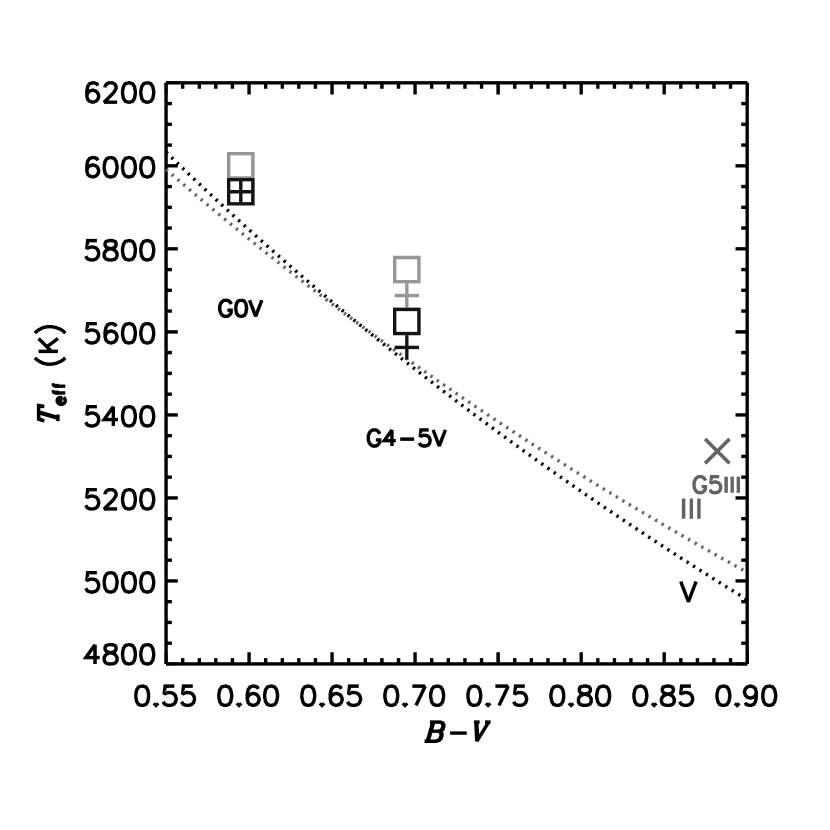
Figure 13: Same as Fig. 10, but for the dwarfs, calibration of RM05 only. For comparison we also show the RM05 calibration for giants (lighter dotted line), and our blue band NLTE result for the G5 III sample.

Table 1: List of spectral class/$[{{\rm A}\over{\rm H}}]$ samples, with the number of stars used to form each sample, the mean (and RMS) $B-V$ value of the stars comprising the sample (from (Mermilliod, 1991)), the total number of $[{{\rm A}\over{\rm H}}]$ values in the Cayrel et al. (2001) catalog among the stars comprising the sample, and the number of individual spectra used to form each sample (the entry in column 5 is larger than that of column 2 when one or more stars in the sample has more than one independenet spectrum in the B85 catalog).

Spectral	Num	Mean	Num	Num
type	stars	$B-V(\sigma)$	[${{\rm A}\over{\rm H}}$]	spectra
G5 III	2	0.882 (0.019)	3	3
G8 III	6	0.930 (0.004)	8	8
K0 III	10	1.043 (0.002)	27	14
K1 III	3	1.115 (0.003)	3	3
K2 III	2	1.160 (0.006)	3	3
K3-4 III	4	1.408 (0.014)	5	4
G0 V	2	0.595 (0.004)	11	2
G5 V	2	0.695 (0.010)	7	2
G8 III	2	1.010 (0.000)	4	3
K1.5 III	1	1.211 (0.009)	17	3

Table 2: LTE models: Closest match models to mean sample spectra and goodness of fit statistics.

	Total SED			Blue			Red
Spectral type	$T_{\rm eff}$	$\log g$	$\sigma_{\rm Min}$	$T_{\rm eff}$	$\log g$	$\sigma_{\rm Min}$	$T_{\rm eff}$	$\log g$	$\sigma_{\rm Min}$	$[{{\rm A}\over{\rm H}}]$
G5 III	5375a	2.0	0.042	5375	2.0	0.062	5250a	3.0	0.023	0.0
G8 III	5125	2.0	0.034	5125	2.0	0.058	5125	2.0	0.011	0.0
K0 III	4875	1.5	0.046	4875	1.5	0.075	4875	2.0	0.022	0.0
K1 III	4562.5	3.0	0.068	4562.5	3.0	0.114	4625	2.5	0.017	0.0
K2 III	4500	2.0	0.056	4500	2.0	0.094	4500	2.0	0.019	0.0
K3-4 III	4250	1.25	0.095	4250	1.25	0.154	4187.5	1.0	0.032	0.0
G0 V	5937.5	4.0	0.035	5937.5	4.0	0.059	6000	5.0	0.013	0.0
G4-5 V	5625	4.0	0.052	5625	4.0	0.078	5750	5.0	0.028	0.0
G8 III	4750	2.0	0.050	4750	2.0	0.077	4625	2.5	0.016	-0.5
K1.5 III	4312.5	1.0	0.069	4187.5	2.0	0.117	4312.5	1.0	0.023	-0.5

Table 3: NLTE models: Same as Table 2.

	Total SED			Blue			Red
Spectral type	$T_{\rm eff}$	$\log g$	$\sigma_{\rm Min}$	$T_{\rm eff}$	$\log g$	$\sigma_{\rm Min}$	$T_{\rm eff}$	$\log g$	$\sigma_{\rm Min}$	$[{{\rm A}\over{\rm H}}]$
G5 III	5312.5a	2.0	0.042	5312.5	2.0	0.063	5250a	3.0	0.022	0.0
G8 III	5062.5	2.0	0.034	5062.5	2.0	0.058	5062.5	2.0	0.010	0.0
K0 III	4812.5	1.5	0.044	4812.5	1.5	0.069	4812.5	2.0	0.021	0.0
K1 III	4562.5	2.5	0.069	4500	3.0	0.114	4562.5	2.0	0.016	0.0
K2 III	4500	2.0	0.057	4500	2.0	0.095	4437.5	1.5	0.020	0.0
K3-4 III	4187.5	1.5	0.094	4187.5	1.5	0.154	4125	1.0	0.031	0.0
G0 V	5937.5	4.0	0.036	5937.5	4.0	0.060	5937.5	4.5	0.012	0.0
G4-5 V	5625	4.0	0.053	5562.5	4.0	0.081	5687.5	5.0	0.028	0.0
G8 III	4687.5	2.0	0.050	4687.5	2.0	0.078	4562.5	2.5	0.015	-0.5
K1.5 III	4187.5	1.5	0.073	4187.5	1.5	0.120	4250	1.25	0.023	-0.5

Table 4: Comparison with less model-dependent $T_{\rm eff}$ calibrations of RM05 and B10.

		LTE		NLTE
Spectral type	B-V    ($\sigma$)	Blue	Red	Blue	Red	RM05	B10
G5 III	0.882 (0.019)	5375	$\cdots$	5312.5	$\cdots$	5137	$\cdots$
G8 III	0.930 (0.004)	5125	5125	5062.5	5062.5	4964	$\cdots$
K0 III	1.043 (0.002)	4875	4875	4812.5	4812.5	4721	$\cdots$
K1 III	1.115 (0.003)	4562.5	4625	4500	4562.5	4592	4737
K2 III	1.160 (0.006)	4500	4500	4500	4437.5	4531	4562
K3-4 III	1.408 (0.014)	4250	4187.5	4187.5	4125	4118	4134
G0 V	0.595 (0.004)	5937.5	6000	5937.5	5937.5	5864	$\cdots$
G4-5 V	0.695 (0.010)	5625	5750	5562.5	5687.5	5519	$\cdots$
G8 III-0.5	1.010 (0.000)	4750	4625	4687.5	4562.5	4684	$\cdots$
K1.5 III-0.5a	1.211 (0.009)	4187.5	4312.5	4187.5	4250	4332	4386

References

- Alonso et al. (2001) Alonso, A., Arribas, S., Martinez-Roger, C., 2001, A&AS, 376, 1039
- Anderson (1989) Anderson, L.S., 1989, ApJ, 339, 558
- Asplund (2000) Asplund, M., 2000, A&A, 359, 755
- Asplund et al. (2004) Asplund, M., Grevesse, N., Sauval, A.J., Allende Prieto, C. & Kiselman, D., 2004, A&A, 417, 751
- Baines et al. (2010) Baines, E.K., Dollinger, M.P., Cusano, F., Guenther, E.W., Hatzes, A.P., McAlister, H.A., ten Brummelaar, T.A., Turner, N.H., Sturmann, J., Sturmann, L., Goldfinger, P.J., Farrington, C.D., & Ridgway, S.T., 2010, ApJ, 710, 1365 (B10)
- Burnashev (1985) Burnashev V.I., 1985, Abastumanskaya Astrofiz. Obs. Bull. 59, 83 (B85)
- Casagrande et al. (2010) Casagrande, L., Ramirez, I., Melendez, J., Bessell, M., & Asplund, M., 2010, A&A, 512, A54
- Cayrel et al. (2001) Cayrel de Strobel, G., Soubiran C., Ralite N., 2001, A&A, 373, 159
- Chiavassa et al. (2010) Chiavassa, A., Collet, R., Casagrande, L., & Asplund, M., 2010, A&A, 524, 93
- Gray (1982) Gray, D.F., 1982, ApJ, 262, 682
- Grevesse et al. (1992) Grevesse, N., Noels, A., Sauval, A.J., 1992, In ESA, Proceedings of the First SOHO Workshop, p. 305
- Hauschildt et al. (1999) Hauschildt, P.H., Allard, F., Ferguson, J., Baron, E. & Alexander, D.R., 1999, ApJ, 525, 871
- Helling et al. (2008) Helling, Ch., Ackerman, A., Allard, F., Dehn, M., Hauschildt, P., Homeier, D., Lodders, K., Marley, M., Rietmeijer, F., Tsuji, T., Woitke, P., 2008, MNRAS, 391, 1854
- Hoffleit & Warren (1991) Hoffleit, E.D., Warren, Jr. W.H., “The Bright Star Catalogue, 5th Revised Ed., 1991, Astronomical Data Center, NSSDC/ADC (BSC5)
- Jacoby et al. (1984) Jacoby, G.H., Hunter, D.A. & Christian, C.A., 1984, ApJS, 56, 257
- Keenan & Barnbaum (1999) Keenan, P.C. & Barnbaum, C., 1999, ApJ, 518, 859
- Keenan & McNeil (1989) Keenan,P.C. & McNeil R.C., 1989, ApJS, 71, 245
- Keenan & Newsom (2000) Keenan,P.C. & Newsom, G.H., 2000, The Revised Catalog of MK Spectra Types for the Cooler Stars, www.astronomy.ohio-state.edu/MKCool/
- Kurucz (1992) Kurucz, R.L., 1992, Rev. Mex. Astron. Astrofis., 23, 181
- Mermilliod (1991) Mermilliod, J.C., 1991, “Catalogue of Homogeneous Means in the UBV System”, Lausanne
- Mishenina et al. (2006) Mishenina, T.V., Bienayme, O., Gorbaneva1, T.I., Charbonnel, C., Soubiran, C., Korotin, S.A. & V. V. Kovtyukh, V.V., 2006, A&A, 456, 1109
- Pinsonneault et al. (2011) Pinsonneault, M.H., An, D., Molenda-Zakowicz,J., Chaplin, W.J., Metcalfe, T.S. & Bruntt, H., 2011, arXiv:1110.4456v1 [astro-ph.SR]
- Ramirez & Melendez (2005) Ramirez, I. & Melendez, J., 2005, ApJ, 626, 446 (RM05)
- Rutten (1986) Rutten, R.J., 1986, in IAU Colloquium 94, Physics of Formation of Fe II lines outside LTE, ed. R. Viotti (Dordrecht: Reidel), p. 185
- Short & Hauschildt (2010) Short, C.I. & Hauschildt, P.H., ApJ, 718, 1416 (Paper I)
- Short & Hauschildt (2009) Short, C.I. & Hauschildt, P.H., 2009, ApJ, 691, 1634
- Short & Hauschildt (2005) Short, C.I. & Hauschildt, P.H., 2005, ApJ, 618, 926
- Short & Hauschildt (2003) Short, C. I. & Hauschildt, P. H. , 2003, ApJ, 596, 501
- Skiff (2010) Skiff, B.A., 2010, General Catalogue of Stellar Spectral Classifications, Lowell Observatory
- Takeda, et al. (2008) Takeda, Y., Sato, B. & Murata, D., 2008, Publ. Astron. Soc. Japan 60, 781
- Vernazza, et al. (1981) Vernazza, J.E., Avrett, E.H. & Loeser, R., 1981, ApJS, 45, 635
- Wang et al. (2011) Wang, L., Liu, Y., Zhao, G. & Sato, B., arXiv:1109.6742v1 [astro-ph.SR]