The workings of the Maximum Entropy Principle in collective human behavior

Abstract

We exhibit compelling evidence regarding how well does the MaxEnt principle describe the rank-distribution of city-populations via an exhaustive study of the 50 Spanish provinces (more than 8000 cities) in a time-window of 15 years (1996-2010). We show that the dynamics that governs the population-growth is the deciding factor that originates the observed distributions. The connection between dynamics and distributions is unravelled via MaxEnt.

I Introduction

Orderliness, reflected in either scaling properties bat1 or power laws city1 ; power ; pareto , is encountered in different frameworks involving social groups. Salient example is Zipf’s law zipf , a power law with exponent $-2$ for the density distribution function that is observed in describing urban agglomerations ciudad and firm sizes all over the world firms . This kind of “order” has got immense attention in the literature. The pertinent regularities have been found in other scenarios as well, ranging from percolation theory and nuclear multi-fragmentation perco to the abundances of genes in various organisms and tissues furu , the frequency of words in natural languages zipf ; zip , the scientific collaboration networks cites , the total number of cites of physics journals nosotrosZ , the Internet traffic net1 or the Linux packages links linux . Another special regularity in the density distribution function of the number of votes in the Brazilian elections,elec1 a power law with exponent $-1$. This kind of distribution is the origin of the so-called First-Digit Law, or Benford’s Lawbenford . Such exponent has also been found in Ref. nosotros, by recourse to an information-theoretic methodologyalp , for both the city-size distribution of the province of Huelva (Spain) and the results of the 2008 Spanish General Elections. Also log-normal distributions are applied to cities’ sizes. While a city-size distribution is often associated with Zipf’s law, this holds only in the upper tail. However the entire distribution of cities, not just the largest ones, is close to log-normal (see Ref. gibrat, ). Undoubtedly, some aspects of human behavior reflect a kind of “universality”.

Common to all these disparate systems is the lack of a characteristic size, length or frequency for the observable of interest, which makes it scale-invariant. In Ref. nosotros, we have introduced an information-theoretic technique based upon the minimization of Fisher’s information measurealp (abbreviated as MFI) that allows for the formulation of a “thermodynamics” for scale-invariant systems. The methodology establishes an analogy between such systems and physical gases which, in turn, shows that the two special power laws mentioned in the preceding paragraph lead to a set of relationships formally identical to those pertaining to the equilibrium states of a scale invariant non-interacting system, the scale-free ideal gas (SFIG). The difference between the two distributions is thereby attributed to different boundary conditions on the SFIG.

Many social systems, however, are not easily included into the two types of description of the preceding paragraph. Inspired in opinion dynamics modelsoppi ; elec1 ; elec2 we described in Ref. oursnow3, a numerical process that reproduces the shapes of the empirical city-population distributions. The model is based in a competitive cluster growth process inside an scale-free ideal network (a scale-free network which degree distribution is described as an SFIG). The finite size of the network introduces competition, and thusly correlations in the cluster sizes. The larger the competitiveness, the larger the deviation from the SFIG distribution. The equivalence with the workings of physical gases is compelling indeed. However, some aspects of the concomitant problems defy full understanding, since an analytical prescription for the classification of the size-distribution of social groups was missing. In order to do look for such analytical understanding we will appeal here to a variational approach centered on information theory.

We have recently shown (see Ref. XXX, ) how to deal with the well-established MaxEnt technique jaynes ; katz by including, within the associated Lagrangian, information regarding equations of motion, i.e., “dynamical” information of a kind that goes beyond the customary one, based upon expectation values. We demonstrated that proportional growth and hyper-exponential growth can both be described in dynamical terms, accurately predicting the equilibrium distribution for such systems. This is tantamount to giving a dynamical interpretation to the ‘information cost’ introduced in Ref. X1, . Our main present purpose is to apply what we learned in XXX, to empirical systems, this demonstrating i) the applicability of MaxEnt to collective human behavior, and ii) the potential use of an explicit social thermodynamics.

This work is is organized as follows: in Sec. II we revisit the theoretical MaxEnt approach to be followed here. In Sec. III we present empirical data for the Spanish provinces. The ensuing results clearly show the usefulness of the theoretical method. In Sec. IV we discuss some noteworthy features of the results an their possible uses in other contexts. A summary is given in Sec. V and, finally, some technical aspects are the subject of the Appendix.

II Theoretical approach

II.1 Basics

Following the methodology described in XXX, , let us define

i)

$N$ as the total population,

ii)

$n_{c}$ as the total number of cities into which people are apportioned,

iii)

$x_{i}$ as the population of the $i$-th city,

iv)

$x_{0}$ as the minimum possible population amount (which is at least $x_{0}=1$),

v)

$p(x)$ as the relative number of cities with exactly a population amount given by $x$.

Considering the continuous limit of the distribution $p(x)$, the conservation of both $N$ and $n_{c}$ guarantees

i)

$\displaystyle\int_{x_{0}}^{\infty}dxp(x)=1$, and

ii)

$\displaystyle\int_{x_{0}}^{\infty}dxp(x)x=N/n_{c}$.

We now turn on MaxEnt: in dynamical equilibrium, the distribution $p(x)dx$ is the one that maximizes Shannon’s entropy $S$ subject to the above constraints. One thereby concocts the variational Lagrangian

$$H=S-\mu n_{c}-\lambda N,$$ (1)

with $\mu$ and $\lambda$ the corresponding Lagrange multipliers. MaxEnt entails $\delta H=0$.

II.2 Dynamics

We showed in Ref. oursnow3, that cities’ population expansion can be modelled by means of clusters’ growth in complex networks. Such process (diffusion) in networks generally starts i) using a node as a seed, ii) its first neighbors being added to the cluster in the first iteration, iii) the neighbors of those neighbors afterwards, and so on. Mathematically, if $\Delta t$ is the interval of time for each iteration and $x(t)$ is the population of the cluster at the time $t$, we can write

$$x_{i}(t+\Delta t)=x_{i}(t)+\Delta t\sum_{j=1}^{x_{i}(t)}k_{j}$$ (2)

where $k_{j}$ is the number of neighbors of the $j$-th node accepted to the cluster per unit time. According to the central limit theorem, we generalize this equation as

$$x_{i}(t+\Delta t)\simeq x_{i}(t)+\Delta t\left(kx_{i}(t)\pm\sigma_{k}\sqrt{x_{i}(t)}\right),$$ (3)

where $k$ is the global mean value of accepted neighbors per unit time and $\sigma_{k}$ its standard deviation. For large enough values of the population this last term can be neglected, and write for the continuous limit

$$\dot{x}_{i}(t)=kx_{i}(t),$$ (4)

where the dot represents the time derivative. This equation represent the so-called proportional growth, whose generalization to a random process leads to the so-called geometrical Brownian motion. We show in Ref. XXX, how to proceed to construct the entropy $S$ for such a scale-free dynamics.

II.3 MaxEnt for scale invariant systems

We now consider a system governed by the proportional growth of Eq. (4), with $k$ being regarded as reflecting a Wiener process. Our equation is linearized by introduction of the new variable $u=\log(x/x_{0})$, which leads to $\dot{u}=k$, and then to a Shannon measure expressed in terms of $u$

$$S=\int_{0}^{\infty}p(u)\log(p(u))du.$$ (5)

With our two conservation rules written now in $u-$terms, the MaxEnt variational problem becomes

$$\delta H=\delta\left[S-\mu\int_{0}^{\infty}dup(u)-\Lambda\int_{0}^{\infty}dup(u)e^{u}\right]=0,$$ (6)

where we have employed the definition $\Lambda=x_{0}\lambda$. The solution is the equilibrium density $p(u)du=Z^{-1}\exp(-\Lambda e^{u})du$, that one now recasts in terms of the observable $x$ getting

$$p(x)dx=Z^{-1}\frac{e^{-\Lambda x/x_{0}}}{x}dx.$$ (7)

From the conservation rules we easily obtain for the pertinent constraints the values

$$\begin{array}[]{c}Z=\Gamma(0,\Lambda)\\ \displaystyle\frac{e^{-\Lambda}}{\Lambda\Gamma(0,\Lambda)}=\frac{N}{n_{c}x_{0}},\end{array}$$ (8)

with $\Gamma(a,z)$ the so-called incomplete Gamma function.

II.4 The Gamma Scaling Law

The concomitant cumulative function $P(x)$ reads

$$P(x)=1-\frac{\Gamma(0,\Lambda x/x_{0})}{\Gamma(0,\Lambda)},$$ (9)

and the associated rank-distribution (RD) —obtained from the inversion of the cumulative one— becomes

$$x=\frac{x_{0}}{\Lambda}\Gamma^{-1}\left[0,\Gamma(0,\Lambda)r/n_{c}\right],$$ (10)

where $r$ is the (continuous) rank from 0 to $n_{c}$, and $\Gamma^{-1}(z)$ denotes the inverse function of $\Gamma:$ $\Gamma(\Gamma^{-1}(z))=z$. We derive from here what we call the Gamma Scaling Law

$$\begin{array}[]{c}\displaystyle x^{\prime}=x\Lambda/x_{0}\\ \displaystyle r^{\prime}=r\Gamma(0,\Lambda)/n_{c},\end{array}$$ (11)

obtaining a “scaled” RD

$$x^{\prime}=\Gamma^{-1}\left(0,r^{\prime}\right),$$ (12)

which no longer depends on $N$, $n_{c}$, or $x_{0}$.

II.5 Beyond proportional growth

We now consider the more general expression

$$\dot{x}(t)=kx^{q}(t),$$ (13)

where $q$ is a dimensionless parameter. Linearization is achieved by means of the q-logarithm of Tsallis’ statisticstsallis

$$\log_{q}(x)=\frac{x^{1-q}-1}{1-q};\,\,\,[x>0;\log_{1}(x)=\ln{x}],$$ (14)

$$e_{q}(x)=[1+(1-q)x]_{+}^{1/(1-q)},$$ (15)

defining the new variable $w=\log_{q}(x/x_{0})$, and so obtaining $\dot{w}=k$. The “$w$”-Shannon entropy becomes

$$S=\int_{0}^{\infty}p(w)\log(p(w))dw.$$ (16)

The concomitant MaxEnt problem is of the form

$$\delta H=\delta\left[S-\mu\int_{0}^{\infty}dup(w)-\Lambda\int_{0}^{\infty}dup(w)e_{q}(w)\right]=0,$$ (17)

whose solution is $p(w)dw=Z^{-1}\exp(-\Lambda e_{q}(w))dw$. Changing back to the observable $x$ we find

$$p(x)dx=Z^{-1}\frac{e^{-\Lambda x/x_{0}}}{x^{q}}dx.$$ (18)

The constraints derive from the conservation rules in the usual manner as

$$\begin{array}[]{c}Z=(\Lambda/x_{0})^{q-1}\Gamma(1-q,\Lambda)\\ \displaystyle\frac{\Gamma(2-q,\Lambda)}{\Lambda\Gamma(1-q,\Lambda)}=\frac{N}{n_{c}x_{0}}.\end{array}$$ (19)

The current cumulative function turns out to be

$$P(x)=1-\frac{\Gamma(1-q,\Lambda x/x_{0})}{\Gamma(1-q,\Lambda)},$$ (20)

and for the associated RD has

$$x=\frac{x_{0}}{\Lambda}\Gamma^{-1}\left[1-q,\Gamma(1-q,\Lambda)r/n_{c}\right].$$ (21)

II.6 Proportional drift in q-exponential growth

We now consider a $q$-equilibrium system subject to a slow proportional drift, that may account for the “natural” population-growth or fluctuations of proportional nature. One is here including a kind of noise that affects the underlying dynamical equation via

$$\dot{x}=k_{1}x+k_{q}x^{q},$$ (22)

or, in terms of $u=\log(x)$,

$$\dot{u}=k_{1}+k_{q}e^{(q-1)u},$$ (23)

where $k_{1}$ characterizes proportional drift and $k_{q}$ hyper-exponential growth. Considering $k_{1}$ also as a Wienner process, the system departs equilibrium via proportional diffusion. As seen in Ref. XXX, , the kernel function for that kind of diffusion is a log-normal distribution. We face the convolution

$$\begin{array}[]{l}p(x;\Lambda,x_{0},q,\sigma)dx=\\ \displaystyle\frac{dx}{(\Lambda/x_{0})^{q-1}\Gamma(1-q,\Lambda)}\int_{x_{0}}^{\infty}dx^{\prime}\frac{e^{-\Lambda x^{\prime}/x_{0}}}{x^{\prime q}}\frac{e^{-\log^{2}(x^{\prime}/x)/2\sigma^{2}}}{x\sqrt{2\pi}\sigma},\end{array}$$ (24)

where $\sigma$ is the drift-scale parameter. The mean value reads

$$\frac{\Gamma(2-q,\Lambda)}{\Lambda\Gamma(1-q,\Lambda)}e^{\sigma^{2}/2}=\frac{N}{n_{c}x_{0}}.$$ (25)

III Empirical observations

III.1 Description of the data used in this work

The raw data are obtained from the Spanish state institute INE and cover annually the period 1996-2010 (with the exception of 1997). It encompasses up to 8000 municipalities (the smallest Spanish administrative unit) distributed within 50 provinces (the building blocks of the autonomous communities, equivalent of the USA-states). The autonomous cities of Ceuta and Melilla are not included. We use provinces and municipalities as the closest representatives of the ideal of a closed system’s fundamental elements. But some arbitrariness remains in the data, since i) there are many municipalities that actually contain more than one population-center, ii) provinces that contains more than a single socioeconomic cluster, and iii) economic regions that extend beyond the frontiers of a province. Those facts introduce systematic errors into the data, but we retain enough accuracy for the purposes of this work.

The appropriateness of provinces as the proper scale for the analysis of this work is due to a trade-off between large enough data sets and locality. Autonomous communities as a whole provide a large enough sample, but the statistical properties we are interested in change within them. Smaller administrative units called comarcas have a more local nature, but only contains a few municipalities and thus introduce large numerical errors. We consider that choosing the adequate scale is the most important ingredient for an study of the kind we attempt here.

The data cover a total Spanish population of 39106917 inhabitants in 1996, reaching 47254510 in 2010. For this last year, the largest municipality (Madrid) covers 3273049 people and the smallest one just 5 persons (Illán de Vacas, Toledo). The total population of each province, $N$, ranges between 6458684 inhabitants (Madrid) and 95258 (Soria), and the number of municipalities, $n_{c}$, between 371 (Burgos) and 34 (Las Palmas). These $n_{c}-$figures are not large enough to build up an accurate density distribution. Accordingly, we have systematically worked with RD instead. RD are usually built from the vector $\mathbf{x}=\{x_{i}\}_{i=1}^{n_{c}}$, where $x_{i}$ is the population of the $i$-th municipality. We assign rank numbers ranging from 1 to $n_{c}$, from the largest ($\max(\mathbf{x})\rightarrow r=1$) to the lowest (in population) ($\min(\mathbf{x})\rightarrow r=n_{c}$). In order to compare with theoretical, continuous rank-distributions, we have found it to be more accurate to assign “middle-point” values from $r=0.5$ to $r=nc-0.5$, instead.

For our analysis we generate, for each province and for each time-period, the pair $(u_{i},\dot{u}_{i})$, with the logarithm of the population $u_{i}$ correlated with the relative population-increment $\dot{u}_{i}$. They are computed as

$$\begin{array}[]{l}\displaystyle u_{i}=\log[x_{i}(t_{2})x_{i}(t_{1})]/2\\ \displaystyle\dot{u}_{i}=\frac{\log[x_{i}(t_{2})/x_{i}(t_{1})]}{t_{2}-t_{1}},\end{array}$$ (26)

where $t_{1}$ and $t_{2}$ are consecutive years for which data are available.

III.2 Zeroth order approximation: proportional growth

III.2.1 A paradigmatic example: Alicante

We use as paradigmatic example the province of Alicante to illustrate our empirical analysis. The inset in the top panel of Fig. 1 depicts $u$ versus $\dot{u}$ for all our municipalities in the last 15 years. The correlation coefficient between the two variables is found to be $0.16$, small enough to consider, at zeroth order approximation, that the growth is of proportional nature, independently of the size, thus obeying Eq. (4).

As seen in the previous section, the equilibrium rank-density predicted for proportional growth by MaxEnt follows Eq. (7), where $\Lambda$ is univocally determined by Eq. (8) with i) an estimated minimum size $x_{0}$, ii) the given total population $N=1926285$ (in 2010) and, iii) the number of municipalities $n_{c}=141$. $N$ and $n_{c}$ are well determined in all cases. In assigning $x_{0}$, fluctuations have an important influence. The easier way of estimating it is via extrapolation (in the rank-plot) of a linear fit to the logarithm of the lowest populations. A more sophisticated method employs a non-linear fitting of the raw data to the MaxEnt rank-distribution via this single parameter, using Eq. (10) together with the definition of $\Lambda$ Eq. (8). Such simple procedure in the log-scale works nicely enough. Note that $\log(x_{0})$ is just a shift of the distribution as a whole, playing no role in its actual shape. We have obtained $\log(x_{0})=4.826$ ($x_{0}=125$), with an standard error of 0.036 and a correlation coefficient of $R=0.99968$. The comparison of the raw data with the analytical rank-distribution is displayed in the top panel of Fig. 1. The shadowed area represents the 90% confidence interval due to finite size effects for $n_{c}=141$, numerically estimated, as described in the Appendix. Since the empirical rank-distribution falls inside the confidence interval, and the observed dynamics are compatible with the dynamical assumption of Eq. (4), we consider that this case constitutes strong evidence for the applicability of the MaxEnt principle.

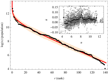
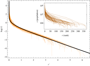
Figure 1: Top panel: Rank-distribution of the province of Alicante (2010), compared with the MaxEnt prediction for proportional growth using the actual total population $N=1926285$ and the estimation $x_{0}=125$. The shadowed area represents the 90% confidence interval for $n_{c}=141$ (2010). Inset: relative change vs. natural logarithm of the population for this province for the last 15 years, where each gray dot represents one municipality for each annual period. Black dots denote the mean value in each interval $\Delta u=1$ and the error bars the standard deviation at that interval. Bottom panel: Gamma-scaled rank-distribution of all 50 provinces. Inset: raw data (2010).

III.2.2 More detailed analysis

We have applied the same (zeroth order) approximation of proportional growth to the rest of Spain’s provinces, also including the values of the total populations $N$ in the fitting procedure. Using the corresponding values of $n_{c}$ together with the estimated values of $x_{0}$ and $N$ we get the value for $\Lambda$, and apply then the Gamma-scaling law described in the previous Section. The scaled rank-distributions are displayed in Fig. 2 (raw data in the inset), and the numerical values of the fitted results can be found in the Additional MaterialAM . A quite nice adjustment ensues in general (correlation coefficient of $R=0.99984$ for Tenerife) but not in all instances ($R=0.99635$ for Guadalajara). This “failure” is linked to the strong correlations between $\dot{u}$ and $u$ for some provinces, that reaches significant values (of up to $R=0.57$ for the province of Lugo). Although such correlations may compromise the validity of the zeroth order approximation of proportional growth, the quite nice scaling-features exhibited by this plot are remarkable indeed.

It is worth mentioning that the fitted value for the total population is found to be systematically lower than the actual value for it. Such scenario usually changes when the capital city of the province is not considered in the fitting process, and thus in the estimation of $N$. This indicates that the population of the capital city is systematically larger than what one would expect from the MaxEnt prediction (off the 90% confidence level). This is not surprising since, as mentioned above, provinces are not ideal, isolated systems: the actual administrative municipality for capital cities are usually the sum of the historical ones plus some near neighbors, and their economy is expected to be highly correlated with that of other capital cities. Although only 50 cities is a small sample, we have studied the rank-distribution of these capitals and their dynamics to shed some light onto this observation. We have found the pleasing result that these capitals form a scale-free system of their own. Comparing the rank-distribution with the MaxEnt prediction that uses i) the actual value $N=15528025$ with ii) the only fitting parameter $\log(x_{0})=10.80\pm 0.05$ ($R=0.99989$, higher than that of Alicante) and encounter that all the 50 cities get located inside the confidence level. When studying the relative increment $\dot{u}$ vs. the log-size $u$, we find a very low size-dependencies ($R=0.15$, lower than the one prevailing for Alicante). This observation confirms the appropriateness of a proportional growth dynamics. Again, the capital city of Madrid exhibits a larger-than-expected population (just in the limit of the 90% confidence level), indicating the possible existence of a higher, international system of correlations.

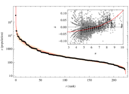
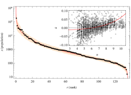
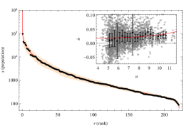
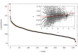
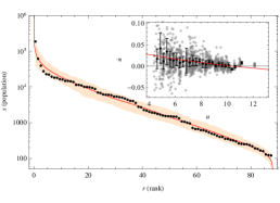
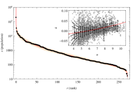
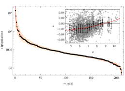
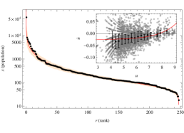
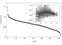
Figure 2: Rank-distribution for Valladolid, Castellón, Girona, Burgos, Guipúzcoa, Navarra, León, Ávila, and Barcelona (year 2010), compared with the pertinent MaxEnt prediction. The shadowed area represents the 90% confidence interval for each $n_{c}$ value. Insets: relative growth vs. logarithm of the population, same as inset of top panel in Fig. 1 but with $\Delta u=0.25$.

III.3 Higher order approximation

III.3.1 Preliminaries

Let us proceed now to tackle a power-law growth by assuming some kind of dependence of $\langle\dot{u}(u)\rangle$ on $u$. Starting from the simplest, linear relation, the idea is to consider an exponential function and its expansion

$$\dot{u}\simeq a+bu\simeq k_{1}+k_{q}e^{(q-1)u},$$ (27)

which is equivalent to Eq. (23). We thus face a “q-dynamics” with proportional noise, whose distribution derives from MaxEnt for $q\neq 1$ Eq. (24).

We confirm, a posteriori, that this procedure is adequate up to $q=2$, evidencing more information than what one would get from just a first order relationship. The actual $q-$value can be determined directly either from the dynamical data or from the rank-distributions. We can demonstrate via MaxEnt that a cause-effect relationship exists between the dynamics and the city-population distribution, if the two kinds of estimations do match (within standard errors).

We have estimated the parameters $x_{0}$, $\Lambda$, $q$, and $\sigma$ of Eq. (24) for each province from the rank-distribution using the methods described in the Appendix, and also, now from the dynamics, the $q$-value for the last 15 years. We find (mean value $\pm$ standard deviation): $\log(x_{0})\sim 5.5\pm 1.3$; $\log(\Lambda)\sim-4.3\pm 1.6$; $q\sim 1.20\pm 0.45$; and $\sigma\sim 0.43\pm 0.24$.

III.3.2 Casuistics

As a general trend, we can fit the rank-distribution with no too many technical complications. In many cases the capital city has to be excluded, as found in the previous subsection. Also, in some other instances, a few of the largest cities have to be excluded. We have also found ‘outsiders’ for very low-population centers. More details are described in the Appendix.

We encounter a strong correlation between the number of municipalities $n_{c}$ and the minimum size $x_{0}$ ($R=-0.77$ for $\log(n_{c})$ vs. $\log(x_{0})$). In similar fashion as for USA (from East to West), the area of the Spanish’ territories grows form North to South, due to historical reasons.

Proportional drift noise, scaled by $\sigma$, has shown to be negligible in some cases but quite important in others. An low correlation is found with $\log(x_{0})$ ($R=-0.15$), but it is largely dependent on $q$ and $\log(\Lambda)$ ($R=0.27$ and $R=-0.40$). Also, the correlation between $q$ and $\log(\Lambda)$ is rather important ($R=-0.37$).

The dynamics’ fit presents some preliminary difficulties. The main one is high noise for low city-sizes (the cause can be found in the last term of Eq. (3), that can not be neglected). Since the mean value of this noise is zero, we have found it compelling to estimate $q$ via the ‘local’ mean value of $\dot{u}$ in Eq. (23), expressed as a function of $u$ (see Appendix)

$$\langle\dot{u}\rangle(u)=\langle k_{1}\rangle+\langle k_{q}\rangle e^{(q-1)u}.$$ (28)

Remarkably enough, we systematically find here a better correlation than for the simple linear fitting. In few cases, even if the variance of $k_{q}$ is large, troubles arise when the value of $\langle k_{q}\rangle$ is small in relation to the drift. In these cases the convergence of the fit falls down to the generic result $q=1$ and an accurate estimation of $q$ cannot be achieved from the dynamics.

III.3.3 Results

We show in Fig. 2 some interesting examples of rank-distributions (plots for all provinces are found in the additional materialAM , and also the table with all the numerical values). Most of the provinces follow quite well the analytical curve, with very few exceptions (the most dramatic of those exceptions correspond to Salamanca, Orense, and Zamora, where a few cities account for the main part of the province’s total population and the small villages follow a log-normal distribution). In general, better fits are obtained for those provinces for which the distributions’ evolution during the last 15 years has been smooth and slow. High rates of change correlate with high $\sigma$. This rather surprising result tells us that if the system is able to reach dynamic equilibrium, it converges to the MaxEnt prediction. We plot in Fig 3 the evolution of $q$ for some examples, that clearly display the correlation we are concerned with here.

Figure 3: Evolution of $q$ via MaxEnt distributions for Alicante (circles), Guipúzcoa (squares), Girona (diamonds), and Navarra (triangles). Alicante is the province with larger $\sigma$ ($0.15$) of these four examples, correlated with its larger time-variation.

We depict in Fig. 4 the comparison between both independent sources for $q$, MaxEnt vs. dynamics, which represent the main result of this work (we display in grey the cases where the dynamical fit fails, near the dynamical value $q=1$). We find a mean proportionality of $0.85$ with a correlation of $R=0.97$. In such instances the dynamical process determines the rank-distribution of the city-population. The equilibrium distribution is that found via maximization of the Shannon entropy in the terms discussed above.

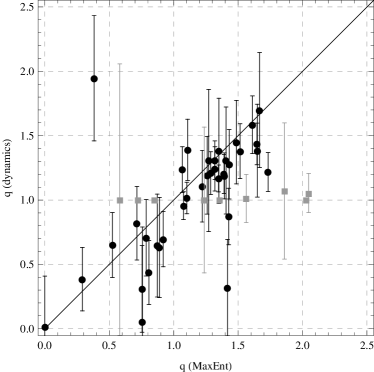
Figure 4: Comparison of measures of $q$, via the comparison MaxEnt distribution vs. dynamics. (gray color represents those cases where the dynamical fit fails, see text).

IV Further remarks

IV.1 Origin of the $q$-dynamics

In the previous section we have successfully parameterized the dynamics without discussing possible underlying mechanisms. We have encountered two general situations:

• i) migration from small villages to big cities and

• ii) saturation of big cities.

The cases of Ávila, Castellón, Valladolid and Navarra constitute nice examples of the first scenario, the most frequent for Spain’s provinces. We usually find for them a value $q>1$. Many examples share for few of the largest cities the second possibility, with a relative growth lower than expected. An explanation for this situation can be found in the finiteness of the resources to make grow a city, thusly avoiding arbitrary large growth rates. Anyhow we have found some examples, as shown for Guipúzcoa, where all the cities follow the second trend and finding values of $q<1$. These cases clearly indicate a generalized migration form cities to small towns, due to some local socioeconomic paradigm.

In other remarkable cases both situations arise in the same region, as happens for Madrid and Barcelona. This is a mark of non-monotonic behavior for $\dot{u}$ with respect $u$, which in such instance compromises the dynamical fit (shown here for Barcelona and in the Additional Material for MadridAM ). On the other hand, the case of Girona deserves some words. Even if it presents a tiny migration-tendency, the system is very near total equilibrium, with an excellent fit for the rank-distribution.

The use of power laws to model both migration and saturation is here of a heuristic nature. We have no evidence of any ‘microscopic’ mechanism generating them, and the value of $q$ is merely obtained from empirical observation. Identifying the mechanism that generates the dynamics constitutes a formidable challenge. It is worth mentioning that growth with saturation has been traditionally modelled using the so-called logistic function, [or its generalization $Y(t)$] with parameters $\alpha$, $K$, and $\nu$ that follow a differential equation of the typewikiglf

$$\dot{Y}(t)=\alpha\left\{1-\left(Y(t)/K\right)^{\nu}\right\}Y(t),$$ (29)

which formally is identical to Eq. (23). Accordingly, migration and growth with saturation generates hyper-exponential growth, but, as far as we know, a pure theoretical determination of the $q$-value from the underlying mechanism is still unknown.

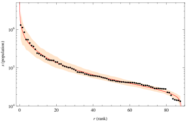
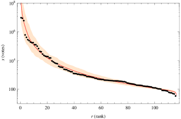
Figure 5: Same as Fig. 2 for the state of Ohio (USA) in 2010 (top), and the general electoral results in United Kingdom in 2005 (bottom).

IV.2 The equation of state

We have shown that the quantities $q$, $\Lambda$, and $\sigma$ exhibit strong correlations amongst themselves, but not with $x_{0}$. MaxEnt gives a relationship between these parameter in the form of Eq. (25), which might be read as an equation of state that relates all of them. The lack of an important correlation with $x_{0}$ is explained because it is a proportionally constant, being just a shift in the log-scale. Since we are dealing with scale invariant systems, the physics does not depend on scale, and the equilibrium distributions respect this fact. The above correlations may indicate the appropriateness of using such equation of state in future city-population research and thermodynamic-oriented analysis.

IV.3 Beyond Spanish cities’ population

We have also found evidences of MaxEnt equilibrium both in other countries and in other kind of social systems, as electoral results, in the present and past years. As an example we plot in the top panel of Fig. 5 the rank-distribution with theoretical fit for the state of Ohio ($\log(\Lambda)=-3.7$, $q=1.62$, $\log(x_{0})=10.1$ and $\sigma=0.36$). We also show in the bottom panel the electoral results for the 2005 UK general elections ($\log(\Lambda)=-13.5$, $q=1.30$, $\log(x_{0})=4.15$ and $\sigma=0.05$). Deeper understanding of each territory/election, correlated with the kind of study presented here may help to better appreciate the effects of regional policies. Work along such lines is in progress.

V Summary

We have shown that the observed city-population distributions of the Spanish provinces follow in general the predicted MaxEnt equilibrium distributions, according to their intrinsic growth dynamics.

• We first have considered a zero-th order approach to the problem assuming proportional growth, thus finding that the empirical distributions can be nicely scaled following the Gamma Scaling Law, derived from the equilibrium distribution of an scale-free system.

• Secondly, we have considered hyper-exponential growth with some proportional drift. We can account in this way for both migration and ‘natural’ growth of the population, obtaining better fits than in the first case.

We have checked that the value of the exponent for the hyper-exponential growth, estimated from the rank-distributions, is equivalent to the one estimated directly from the dynamics, which we read as a confirmation of the validity of our approach.

ACKNOWLEDGMENT: This work was partially supported by ANR DYNHELIUM (ANR-08-BLAN-0146-01) Toulouse, and the Projects FQM-2445 and FQM-207 of the Junta de Andalucía. AP acknowledges support from the Senior Grant CEI Bio-Tic GENIL-SPR.

Appendix A Estimation of the MaxEnt distribution parameters from empirical rank-distributions

A.1 Estimation of the distribution’s 90% confidence interval

The confidence levels of the rank-distributions for a given number $n_{c}$ are estimated as follows:

i)

A list of $n_{c}$ random numbers is generated, following the desired distribution, by inverse transform sampling.

ii)

The list is sorted from largest to lowest $n_{c}$ in order to obtain the rank-distribution. The list is saved for further use.

iii)

A large number of lists is generated following i) and ii), obtaining a distribution of numbers for each element of the list.

iv)

The 0.95-th and 0.05-th quartiles are obtained from the distribution for each element, determining the lower and upper limits of the 90% confidence interval.

A.2 Fit for q-exponential growth

A first method to estimate the MaxEnt q-distributions’ parameters $\Lambda$, $x_{0}$, and $q$ for a given empirical data is a direct fit of the rank-distribution to Eq. (21). We have used the Mathematica softwaremath to this end, by means of the NonlinearModelFit function using different guesses for the initial values. We also compare the pertinent results with a solution obtained from the reproduction of the first three moments of the distribution, finding, statistically and numerically, better stability using the logarithmic moments $\langle(\log(x/x_{0}))^{n}\rangle$ instead of $\langle(x/x_{0})^{n}\rangle$. We have tabulated them as functions of $q$ and $\Lambda$ in the form $M_{n}(q,\Lambda)=\langle[\log(x/x_{0})]^{n}\rangle$, which are defined via

$$\begin{array}[]{rl}\displaystyle\langle\log(x/x_{0})\rangle=&\displaystyle\frac{1}{\Gamma(1-q,\Lambda)}~{}G^{3~{}0}_{2~{}3}\left(\Lambda\left|\begin{array}[]{c}1~{}1\\ 0~{}0~{}(1-q)\end{array}\right.\right)\\ \displaystyle\langle[\log(x/x_{0})]^{2}\rangle=&\displaystyle\frac{2}{\Gamma(1-q,\Lambda)}~{}G^{4~{}0}_{3~{}4}\left(\Lambda\left|\begin{array}[]{c}1~{}1~{}1\\ 0~{}0~{}0~{}(1-q)\end{array}\right.\right)\\ \displaystyle\hfil&\displaystyle\cdots\\ \displaystyle\langle[\log(x/x_{0})]^{n}\rangle=&\displaystyle\frac{n!}{\Gamma(1-q,\Lambda)}G^{(n+2)~{}0}_{(n+1)~{}(n+2)}\left(\Lambda\left|\begin{array}[]{c}1~{}\ldots~{}1\\ 0~{}\ldots~{}(1-q),\end{array}\right.\right)\end{array}$$ (30)

where $G$ stands for the so-called Meijer G-functions. The associated system of equations is

$$M_{n}(q,\Lambda)=E[\log^{n}(x/x_{0})]=\sum_{m=0}^{n}(-1)^{m}\left(\begin{array}[]{c}n\\ m\\ \end{array}\right)E[\log^{n-m}(x)]\log^{m}(x_{0}),$$ (31)

that we deterministically solve using $n=1,2,3$ via $\Lambda$, $x_{0}$, and $q$, with the empirical expected values $E[\log^{n}(x)]=\sum_{i=1}^{n_{c}}\log^{n}(x_{i})/n_{c}$.

We have also introduced into our equations the proportional drift parameterized with $\sigma$. Its inclusion in the above equations can be easily materialized using the additive property of cumulants for convolutions. Remember that the cumulants of a probability distribution (PD) are a set of quantities that provide an alternative to the PD-moments. These, in turn, determine the cumulants in the sense that any two probability distributions whose moments are identical will have identical cumulants as well, and similarly the cumulants determine the moments. In some cases theoretical treatments of problems in terms of cumulants are simpler than those using moments.wikicum Taking into account that for the centered normal distribution only the second cumulant does not vanish, we face the following system of equations

$$\sum_{i=0}^{\lfloor n\rfloor}T^{n}_{i}\sigma^{2i}M_{n-2i}(q,\Lambda)=\sum_{m=0}^{n}(-1)^{m}\left(\begin{array}[]{c}n\\ m\\ \end{array}\right)E[\log^{n-m}(x)]\log^{m}(x_{0}),$$ (32)

where $T^{n}_{i}$ is the $i$-th element of the $n$-th row of the triangle of Bessel numbersseries $T^{n}_{i}=n!/(i!2^{i}(n-2i)!)$.

The ensuing system of equations is solved using the FindRoot functionality of Mathematica with different starting points so as to ensure the best possible result. We accept a set of parameters if the three different results (fit, and equations’ system with/without drift) are reasonably similar. When that does not happen, we look for outsiders, excluding some points from the tails (largest or smallest) until reaching a satisfactory convergency of the three results. The most frequently outsiders-case obtains for the capital city. The second case refers to a few small villages with undersized population. All outsiders are indicated in the Additional MaterialAM , together with the results of the three estimations. On the other hand, as commented in the text, we have found three notorious cases –Salamanca, Orense, and Zamora– where no satisfactory outcome has been achieved with this procedure.

A.3 Fitting the dynamical data

As commented in the text, we have fitted the mean value $\langle\dot{u}\rangle(u)$ to Eq. (28) via $\langle k_{1}\rangle$, $\langle k_{q}\rangle$, and $q$. We have employed again the NonlinearModelFit function, with different guesses for the initial values. The data set for $\langle\dot{u}\rangle(u)$ (and also the standard deviation) is systematically computed in bins of size $\Delta u=0.25$ for all the provinces. Very few points can be found in some of the bins, which introduces high numerical error. Accordingly, we include the bin in the data set if, and only if, a minimal number of points exists. We have assumed, for all the provinces, that this number is the 15% of the bin with the larger number of points. The bins used in each fit are shown in the inset of the rank-distribution plots. Anyhow, this filter is not enough in a few cases, for which a satisfactory result can not be encountered. A $q$-value closed to 1, albeit ill-defined, is the result.

References

- (1) M. Batty, Science 319, 769 (2008).
- (2) A. Blank, S. Solomon, Physica A 287, 279 (2000). X. Gabaix, Y.M. Ioannides, Handbook of Regional and Urban Economics, Vol. 4 (North-Holland, Amsterdam, 2004); W. J. Reed, J. Regional Sci. 42, 1 (2002).
- (3) M.E.J. Newman, Contemp. Phys. 46, 323 (2005).
- (4) V. Pareto, Cours d‘Economie Politique (Droz, Geneva, 1896).
- (5) G.K. Zipf, Human Behavior and the Principle of Least Effort (Addison-Wesley, Cambridge, MA, 1949).
- (6) L.C. Malacarne, R.S. Mendes, E.K. Lenzi, Phys. Rev. E 65, 017106 (2001); M. Marsili, Yi-Cheng Zhang, Phys. Rev. Lett. 80, 2741 (1998).
- (7) R. L. Axtell, Science 293, 1818 (2001).
- (8) K. Paech, W. Bauer, S. Pratt, Phys. Rev. C 76, 054603 (2007); X. Campi and H. Krivine, Phys. Rev. C 72, 057602 (2005); Y. G. Ma et al., Phys. Rev. C 71, 054606 (2005).
- (9) C. Furusawa and K. Kaneko, Phys. Rev. Lett. 90, 088102 (2003).
- (10) I. Kanter and D.A. Kessler, Phys. Rev. Lett. 74, 4559 (1995).
- (11) M. E. J. Newman, Phys. Rev. E 64, 016131 (2001).
- (12) A. Hernando, D. Puigdomènech, D. Villuendas, C. Vesperinas, A. Plastino, Phys. Lett. A 374, 18 (2009).
- (13) R. Albert, A.L. Barabási, Rev. Mod. Phys. 2074, 2047 (2002). M.E.J. Newman, A.L. Barabasi, D.J. Watts, The Structure and Dynamics of Complex Networks (Princeton University Press, Princeton, 2006).
- (14) T. Maillart, D. Sornette, S. Spaeth, and G. von Krogh, Phys. Rev. Lett. 101, 218701 (2008).
- (15) R.N. Costa Filho, M.P. Almeida, J.S. Andrade, and J.E. Moreira, Phys. Rev. E 60, 1067 (1999).
- (16) F. Benford, (March 1938) Proceed. Am. Phil. Soc. 78, 551572 (1938); Weisstein, Eric W., ”Benford’s Law” from MathWorld (http://mathworld.wolfram.com/BenfordsLaw.html).
- (17) H. Rozenfeld, D. Rybski, J. S. Andrade, M. Batty, H. E. Stanley, H. A. Makse, Proc. Nat. Acad. Sci. 105, 18702 (2008).
- (18) A. Hernando, C. Vesperinas, A. Plastino, Phys. A 389, 490 (2010).
- (19) R. Frieden, A. Plastino, A. R. Plastino, and B. H. Soffer, Phys. Rev. E 60, 48 (1999).
- (20) C. Castellano, S. Fortunato, and V. Loreto, Rev. Mod. Phys., 81, 591 (2009).
- (21) S. Fortunato, C. Castellano, Phys. Rev. Lett. 99, 138701 (2007).
- (22) A. Hernando, D. Villuendas, C. Vesperinas, M. Abad, A. Plastino, Eur. Phys. J. B 76, 87 (2010).
- (23) A. Hernando, A. Plastino, A. R. Plastino, MaxEnt and dynamical information, pre-print at arXiv:1201.0889v1 (2012).
- (24) The Additional Material is available at http://sthar.com/uploads/add.pdf.
- (25) E. T. Jaynes, (1957). Phys. Rev. 106, 620 (1957); 108 (1957) 171; IEEE Trans. Syst. Sci. & Cyb. 4, 227 (1968).
- (26) A. Katz, Principles of statistical mechanics: the information theory approach (W. H. Freeman, San Francisco, 1967).
- (27) S. K. Baek, S. Bernhardsson, P. Minnhagen, New J. Phys. 13, 043004 (2011).
- (28) C. Tsallis, J. Stat. Phys. 52, 479 (1988); Phys. Rev. E 58, 1442 (1998); L. Zunino et al., Physica A 388 1985 (2009).
- (29) Wikipedia, http://en.wikipedia.org/wiki/Generalised_logistic_function.
- (30) Mathematica, Wolfram Research Inc. 1988-2011.
- (31) Wikipedia, http://en.wikipedia.org/wiki/Cumulant.
- (32) The On-Line Encyclopedia of Integer Sequences, http://www.oeis.org/A100861.