MaxEnt and dynamical information

Abstract

The MaxEnt solutions are shown to display a variety of behaviors (beyond the traditional and customary exponential one) if adequate dynamical information is inserted into the concomitant entropic-variational principle. In particular, we show both theoretically and numerically that power laws and power laws with exponential cut-offs emerge as equilibrium densities in proportional and other dynamics.

1 Introduction

The principle of maximum entropy is a fundamental idea of contemporary science. It states that, subject to known constraints, the probability distribution which best represents the current state of knowledge is the one with largest entropy jaynes ; katz . In other words, let some testable information about a probability distribution function be given and consider the set of all trial probability distributions that encode this information. The probability distribution that maximizes the information entropy should be regarded as the optimal probability distribution with respect to the a priori available information. In most practical cases, the testable information is given by a set of conserved quantities (average values of some moment functions), associated with the probability distribution in question. This is the way the maximum entropy principle is most often used in statistical thermodynamics. Another possibility is to prescribe some symmetries of the probability distribution. An equivalence between the conserved quantities and corresponding symmetry groups implies the same level of equivalence for both these two ways of specifying the testable information in the maximum entropy method. The maximum entropy principle is also needed to guarantee the uniqueness and consistency of probability assignments obtained by different methods, statistical mechanics and logical inference in particular. The maximum entropy principle makes explicit our freedom in using different forms of prior information. As a special case, a uniform prior probability density (Laplace’s principle of indifference) may be adopted. Thus, the maximum entropy principle is not just an alternative to the methods of inference of classical statistics, but it is an important conceptual generalization of those methods katz .

In this communication we reveal how to accommodate dynamical information into the principle via a special treatment of the equations of motion that considers proportional and larger-than-proportional dynamics due to their importance in the study of complex systems. Some rather surprising results ensue (power-laws and power-laws with exponential cutoffs power ) that illustrate the power of the approach.

We demonstrate that taking into account dynamical information within MaxEnt involves adding to the pertinent Hamiltonian new terms and that these resemble the so-called “information cost” lucidly introduced by the authors of Ref. X1 . In this way we explicitly reconcile two apparent different viewpoints, i.e., that of the growth models of Simon X2 and the information-treatment of Mandelbrot X3 , showing that the equilibrium density of a growth process is the one that maximizes the entropy associated to the enlarged Hamiltonian introduced here.

Our presentation is organized as follows: in Section 2 we present the basics of the problem; in Section 3 we describe the theoretical approach finding the equilibrium densities by means of MaxEnt according to the dynamical equation that governs the system at habd; in Section 4 we confirm our findings by means of numerical experiments with random walkers, and we close drawing some conclusions in Section 5.

2 Preliminary matters

Let us define

i)

$N$ as the total number of elements/members of a discrete set,

ii)

$n_{c}$ as the total number of special subsets into which the $N-$elements can be grouped,

iii)

$x_{i}$ as the number of members of the $i$-th subset,

iv)

$n(x)$ as the total number of subsets with exactly $x$ members.

Considering that $n(x)$ is a discrete distribution, the conservation of both $N$ and $n_{c}$ guarantees

i)

$\displaystyle\sum_{x=1}^{\infty}n(x)=n_{c}$, and

ii)

$\displaystyle\sum_{x=1}^{\infty}xn(x)=N$.

Let us now consider the continuous limit of the distribution $n(x)/n_{c}\rightarrow p(x)dx$.

Our goal here is that of finding out, via MaxEnt, the explicit form of $p(x)dx$ from either some simple expectation-values’ constraints or, and this is the novelty, from dynamical information not of that kind.

3 Theoretical approach

3.1 Brownian motion: the ideal gas

We first consider, as a control case, the dynamics behind the evolution of subsets of sizes $x$ via the linear equation:

$$\dot{x}=k$$ (1)

where $k$ involves a Wiener process, i.e., $\langle k_{i}(t)k_{j}(t^{\prime})\rangle=K\delta_{ij}\delta(t-t^{\prime})$ being $K$ the variance of $k$. We are in the presence of the well-know Brownian motion, which obeys the diffusion equation

$$\partial_{t}p(x,t)=D\partial_{x}^{2}p(x,t),$$ (2)

with $D$ the diffusion coefficient and $p(x,t)$ the non-equilibrium density at instant $t$. Starting at $t=0$ with a Dirac-delta distribution $p(x,0)=\delta(x-x^{\prime})$, the solution to this equation is a gaussian distribution of the form (we set for simplicity $x^{\prime}=0$)

$$p(x,t)=\frac{1}{\sqrt{4\pi Dt}}e^{-\frac{(x)^{2}}{4Dt}}.$$ (3)

The Shannon entropy measure is defined (up to a constant) as

$$S=-\int_{\Omega}dxp(x)\log p(x),$$ (4)

where $\Omega$ is a “volume” in $x-$space defined by a lower and an upper limit of allowed sizes $x_{0}$ and $x_{M}$, respectively ($x_{0}\leq x\leq x_{M}$, thusly $\Omega=x_{M}-x_{0}$,). As our first trial we use just MaxEnt with a normalization constraint

$$\delta\left[S-\mu\int_{\Omega}dxp(x)\right]=0,$$ (5)

where $\mu$ is the associated Lagrange multiplier. The density that extremizes this quantity is the constant one $p(x)dx=Z^{-1}\,dx$ with $Z=\Omega$ the normalization constant (and also by definition the partition function katz ), representing the classical ideal gas —an ensemble of non-interacting particles at constant density and gaussian distribution of velocities. As a second trial we add a constraint on the first moment (the mean value of the sizes) $\langle x\rangle=N/n_{c}$,

$$\delta\left[S-\mu\int_{\Omega}dxp(x)-\lambda\int_{\Omega}dxp(x)x\right]=0.$$ (6)

The concomitant distribution is the well-know exponential density

$$p(x)dx=\frac{\exp(-\lambda x)dx}{Z},$$ (7)

followed by an ideal gas in the gravitational field. Note that $x_{M}$ could diverge here, but $x_{0}$ has a lower bound. The constants $Z$ and $\Lambda=x_{0}\lambda$ (defined for convenience) can be obtained according to

$$\begin{array}[]{c}\displaystyle Z=x_{0}\frac{e^{-\Lambda}}{\Lambda}\\ \\ \displaystyle\Lambda^{-1}+1=\frac{N}{n_{c}x_{0}}.\end{array}$$ (8)

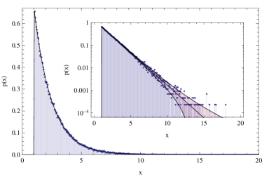
We depict in Fig. 1 an arbitrary case for $x_{0}=1$, $N=250000$ and $n_{c}=100000$ ($\Lambda=1/24$).

Figure 1: Equilibrium density for the $q=0$ case (see Eq. (21) in the text) for $x_{0}=1$, $N=250000$ and $n_{c}=100000$ ($\Lambda=1/24$). Black line: prediction from the MaxEnt, blue dots: histogram of the asymptotic distribution of brownian walkers. The shadowed area in the inset around the line reflects the numerical error of the simulation $O(1/\sqrt{n_{c}})$.

Let us assume that our constraint is a mean-energy-one. Then, the distribution (7) can be associated to a “Hamiltonian” katz

$$H=\Lambda x/x_{0},$$ (9)

and is, for instance, the distribution followed by an ideal gas in the gravitational field. Having a Hamiltonian, it is straightforward to introduce a temperature here by multiplying it by $\beta=1/T$. The partition function defined as $Z=\int dx\,\exp{(-\beta\,H)}$ [Eq. (8)] seemingly remains invariant but with a redefined $\Lambda$ that changes in the fashion $\Lambda\rightarrow\beta\Lambda$.

3.2 Geometric Brownian motion: the scale-free ideal gas

It is well-known that some social and economic systems display a scale-free behavior [see, for instance, oursnow1 ; oursnow2 ; oursnow3 , and references therein]. Thus, we attempt now introducing a proportional growth into the orthodox Jaynes-MaxEnt treatment. We start by considering the equation,

$$\dot{x}=kx$$ (10)

where $k$ is again indicative of a Wiener process, and, of course, we deal here with the very the definition of geometric Brownian motion. We now proceed to linearize the dynamic equation via the new variable $u=\log(x/x_{0})$ obtaining thereby

$$\dot{u}=k.$$ (11)

In analogy with the precedent case, we have the usual Brownian motion for the variable $u$ obeying the diffusion equation. As for the $x$ observable one has

$$\partial_{t}p(x,t)=D\partial_{x}\left(x\partial_{x}\left(xp(x,t)\right)\right),$$ (12)

solved (with an initial Dirac-delta $p(x,0)=\delta(x-x^{\prime})$) via the log-normal distribution (we set for simplicity $x^{\prime}=0$)

$$p(x,t)=\frac{1}{\sqrt{4\pi Dt}x}e^{-\frac{\log^{2}(x)}{4Dt}}.$$ (13)

The Shannon entropy in the variable $u$ is written as

$$S=-\int_{\Omega}dup(u)\log p(u),$$ (14)

with $u$ instead of $x$. The first constraint is expressed, as usual, as

$$\delta\left[S-\mu\int_{\Omega}dup(u)\right]=0,$$ (15)

that yields a constant density for $u$ as $p(u)du=Z^{-1}du$, with $Z=\Omega=\log(x_{M}/x_{0})$. Changing back to the observable $x=x_{0}e^{u}$ we find

$$p(x)dx=\frac{1}{Z}\frac{dx}{x},$$ (16)

which follows the density-behavior of the scale-free ideal gas (SFIG), as found before by means of Fisher’s information in references oursnow1 ; oursnow2 ; oursnow3 .

We remind the reader here of Benford’s law (BL) benford ; benford2 , also called the first-digit law. As shown in Ref. benford2 by means of a bright heuristic derivation, the distribution that originates BL for first digits has the form of Eq. 16. Its occurrence is typical of low self-correlated data with no characteristic size, and thus agrees with the SFIG-definition of a non-interacting system with scale invariance.

Figure 2: Same as Fig. 1 for the $q=1$ case of Eq. (21)

.

The second constraint is now expressed in terms of $u$ via $\langle x\rangle=x_{0}\langle e^{u}\rangle=N/n_{c}$, and the Jaynes-MaxEnt extremization problem becomes

$$\delta\left[S-\mu\int_{\Omega}dup(u)-\Lambda\int_{\Omega}dup(u)e^{u}\right]=0,$$ (17)

where we have used the definition $\Lambda=x_{0}\lambda$. We obtain the density $p(u)du=Z^{-1}\exp(-\Lambda e^{u})du$. Changing back to the observable $x$ we arrive at

$$p(x)dx=\frac{1}{Z}\frac{\exp\left(-\Lambda x/x_{0}\right)}{x}dx.$$ (18)

The pertinent constants are obtained from the constraints in the fashion

$$\begin{array}[]{c}\displaystyle Z=\Gamma(0,\Lambda)\\ \displaystyle\frac{e^{-\Lambda}}{\Lambda\Gamma(0,\Lambda)}=\frac{N}{n_{c}x_{0}},\end{array}$$ (19)

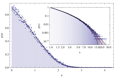
where $\Gamma(a,z)$ is the so-called incomplete Gamma function. This is then the expected equilibrium distribution for an scale-free system, as those of opinion cluster dynamics in networks with fixed number of nodes $N$ as well as the number clusters $n_{c}$ oursnow3 . We display in Fig. 2 the case for the same values of $x_{0}$, $N$ and $n_{c}$ as in the preceding Section (now with $\Lambda=0.360743$).

Assume again that our constrain is a mean-energy-one. We can associate then to the distribution (18) the effective proportional-growth Hamiltonian katz

$$H=\Lambda x/x_{0}+\ln(x/x_{0}),$$ (20)

where the new term $\ln(x/x_{0})$ is the dynamical counterpart of the information-cost of Ref. X1 .

3.3 Q-metric Brownian motion: the generalization to hyper-exponential growth

We now relax the condition of proportional growth and appeal to the more general expression

$$\dot{x}=kx^{q},$$ (21)

where $q$ is a dimension-less parameter. It is easy to see that the two former examples are particular cases corresponding to $q=0$ (Brownian motion) and $q=1$ (geometric Brownian motion). We call this new generalization of the dynamics the q-metric Brownian motion and proceed to a linearization of the dynamic equation by introduction of the variable

$$u=\log_{q}(x/x_{0}),$$ (22)

where $\log_{q}(z)$ is the q-logarithm of Tsallis’ statistics tsallis . One finds

$$\dot{u}=k.$$ (23)

As before, this equation describes the Brownian motion in $u$, and thus a diffusion equation for $x$ of the form

$$\partial_{t}p(x,t)=D\partial_{x}\left(x^{q}\partial_{x}\left(x^{q}p(x,t)\right)\right),$$ (24)

whose solution for an initial Dirac-delta $p(x,0)=\delta(x-x^{\prime})$ is the q-log-normal distribution

$$p(x,t)=\frac{1}{\sqrt{4\pi Dt}x^{q}}e^{-\frac{(\log_{q}(x/x_{0})-\log_{q}(x^{\prime}/x_{0}))^{2}}{4Dt}}.$$ (25)

We keep using Shannon’s entropy in the MaxEnt approach:

$$S=-\int_{\Omega}dup(u)\log p(u),$$ (26)

and the first constraint is expressed, as usual, via

$$\delta\left[S-\mu\int_{\Omega}dup(u)\right]=0,$$ (27)

which yields a constant density for $u$ as $p(u)du=Z^{-1}du$, with $Z=\Omega=\log_{q}(x_{M}/x_{0})$. Now, changing to the observable $x=x_{0}\exp_{q}(u)$ we obtain

$$p(x)dx=\frac{1}{Z}\frac{dx}{x^{q}},$$ (28)

i.e., a power law. We express now the second constraint as $\langle x\rangle=x_{0}\langle\exp_{q}(u)\rangle=N/n_{c}$, writing

$$\delta\left[S-\mu\int_{\Omega}dup(u)-\Lambda\int_{\Omega}dup(u)\exp_{q}(u)\right]=0,$$ (29)

which solution for its extremization is the density $p(u)du=Z^{-1}\exp(-\Lambda\exp_{q}(u))du$. Changing back to the observable $x$ we now get

$$p(x)dx=\frac{1}{Z}\frac{\exp\left(-\Lambda x/x_{0}\right)}{x^{q}}dx.$$ (30)

The associated constants are then obtained from the constraints and one sees that

$$\begin{array}[]{c}\displaystyle Z=(\Lambda/x_{0})^{q-1}\Gamma(1-q,\Lambda)\\ \\ \displaystyle\frac{\Gamma(2-q,\Lambda)}{\Lambda\Gamma(1-q,\Lambda)}=\frac{N}{n_{c}x_{0}}.\end{array}$$ (31)

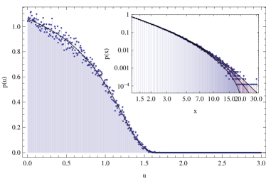
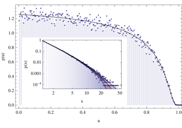
We depict in Fig. 3 the distributions for the same parameters as Figs. 1 and 2 for $q=1.5$ and $q=2$, obtaining $\Lambda=0.223742$ and $\Lambda=0.103808$, respectively.

Figure 3: Same as Fig. 1 for the $q=1.5$ and $q=2$ cases.

Assuming once more time that our constrain is a mean-energy-one, the effective Hamiltonian here reads katz

$$H=\Lambda x/x_{0}\,+q\ln(x/x_{0}).$$ (32)

Again, the new term resembles the information-cost of Ref. X1 . One can introduce once again an inverse “temperature” $\beta$ multiplying the Hamiltonian. The partition function $Z=\int dx\,\exp{(-\beta\,H)}$ turns out to be expressed in terms of the incomplete Gamma function abra

$$Z=(\beta\Lambda/x_{0})^{\beta q-1}\Gamma(1-\beta q,\beta\Lambda).$$ (33)

Comparing with Eq. (31) the partition function $Z$ remains invariant save for a redefinition $q\rightarrow\beta q$ and $\Lambda\rightarrow\beta\Lambda$. Note also that comparing with Eq. (19) we recover the proportional growth partition function at that special temperature for which $\beta=1/q$. Thus, by increasing $T$ from zero to $q$ we can cancel out a dynamical behavior via “heating”. Interestingly enough, in the limit $\beta\rightarrow\infty$ ($T\rightarrow 0$) the equilibrium density distribution is $p(x)dx=\delta(x-x_{0})dx$, i.e., all elements become placed at the same $x_{0}$. The absolute entropy vanishes, as it should (third law of thermodynamics). Actual attainment of the $T=0-$situation would entail a weird configuration indeed, since it seems impossible that $x_{0}$ could accommodate all elements simultaneously.

Figure 4: Diffusion of the initial delta distribution peaked at $x^{\prime}=\langle x\rangle=2.5$, at $\tau=$0.2 (blue), 1.5 (green) and 4 (red) MC steps, with the asymptotic distribution (black) compared with the MaxEnt prediction (black smooth line). Inset: convergence of the standard deviation for the $q=0$ case (see text). The shadowed area here reflects the numerical error $1/\sqrt{n_{c}}$.

4 Numerical experiments and results

4.1 Brownian motion

We have proceeded to confirm our theoretical findings by means of numerical experiments, simulating the dynamics of random walkers following the dynamical equations proposed here. As a control case, we start with the linear $q=0$, largely used in physics in molecular dynamics, statistical mechanics and so on. Our algorithm works as follows:

i)

We firstly fix the minimum $x_{0}$, the number of walkers $n_{c}$ and the mean value $N/n_{c}$. We generate a vector $\mathbf{x}$ with $n_{c}$ elements as $x_{i}=N/n_{c}$, $\forall i$, which represents the walkers.

iii)

We randomly select the $i$-th walker and generate a new position by discretization of the dynamical equation as $x_{i}=x_{i}+kd\tau$, where $k$ is a gaussian random number with variance $K$ and zero mean, and $d\tau$ is an arbitrary small ‘time’ interval.

iv)

We correct the mean value in a way compatible with the dynamical equation, i.e., linearly. A general approach is via the change $\mathbf{x}^{\prime}=\mathbf{x}+\Delta$, where $\Delta=N/n_{c}-\langle x\rangle$. It is worth mentioning that the computational time is reduced by randomly choosing a second $j$-th walker and make it evolve with $x_{j}=x_{j}-kd\tau$ using the same value of $k$ as above. We finally accept the changes if, and only if, $\min(\mathbf{x})\geq x_{0}$.

v)

We repeat iii) and iv) iteratively until achieving convergence in the distribution of $\mathbf{x}$.

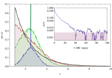
We display in Fig. 5 the diffusion of $n_{c}=100000$ walkers initially peaked at $x=2.5$ ($N=250000$), for different simulation times, at 0.2, 1.5, and 4 Monte-Carlo steps, defining each MC step as $n_{c}$ iterations using $K=1$ and $d\tau=10$. We compare them with the asymptotic equilibrium distribution (also shown in Fig. 1) and depict the convergence of the relative difference of the standard deviation to what is predicted by our MaxEnt treatment, $\varepsilon(\sigma)=|\sigma_{\mathrm{MaxEnt}}-\sigma(\tau)|$. As expected, after some steps we finally reproduce the theoretical MaxEnt distribution. We remark on the importance of correcting the positions of the walkers in linear fashion, respecting the dynamical equation and guaranteeing maintenance of the operative constraint at the main value $\langle x\rangle$.

Figure 5: Same as Fig. 5 for the $q=1$ case, at $\tau=$0.2 (blue), 0.8 (green) and 2.5 (red) MC steps.

4.2 Geometric brownian motion

We have proceeded for $q=1$ in a similar way as in the precedent case, with the difference that now there are two equivalent descriptions for the dynamics involved. The algorithm for the first of them is as follows

i)

We fix the values of $x_{0}$, $n_{c}$ and $N/n_{c}$. We again generate the walkers as a vector $\mathbf{x}$ with $n_{c}$ elements as $x_{i}=N/n_{c}$, $\forall i$.

iii)

We randomly select the $i$-th walker and generate a new position as $x_{i}=x_{i}+kx_{i}d\tau$.

iv)

We now correct the mean value in a way compatible with the dynamical equation, i.e., proportionally. We change $\mathbf{x}^{\prime}=\mathbf{x}\times\Delta$, where now $\Delta=(N/n_{c})/\langle x\rangle$. We accept the changes if, and only if $\min(\mathbf{x})\geq x_{0}$.

v)

We repeat iii) and iv) iteratively until encountering convergence in the distribution of $\mathbf{x}$.

This algorithm solves explicitly the equation of motion in $x$, which requires a specially small time interval $d\tau$ in order to reduce the error in the discretization of the time derivative. The convergence is achieved after a somewhat big computational effort since $d\tau\ll(\sqrt{K}x_{M})^{-1}$. We highly recommend working with the variable $u=\log(x/x_{0})$ to linearize the equations, and apply afterwards the forthcoming algorithm:

i)

We fix the values of $x_{0}$, $n_{c}$, and $N/n_{c}$ to generate the walkers as a vector $\mathbf{u}$ with $u_{i}=\log(N/(n_{c}x_{0}))$, $\forall i$.

ii)

We randomly select the $i$-th walker and generate a new position as $u_{i}=u_{i}+kd\tau$.

iii)

We now correct the mean value as $\mathbf{u}^{\prime}=\mathbf{u}+\Delta$, where now $\Delta=\log[(N/n_{c})/\langle x_{0}\exp(u)\rangle]$ —note that we use now the mean value of the exponential. We accept the changes if, and only if $\min(\mathbf{u})\geq 0$.

iv)

We repeat ii) and iii) iteratively until reaching convergence in the distribution of $\mathbf{u}$.

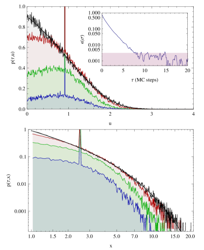
It is easy to see that both algorithms are equivalents since $x_{i}(1+kd\tau)\simeq x_{i}e^{kd\tau}=e^{u_{i}+kd\tau}$. We depict in Fig. 6 the diffusion of the initial delta distribution at 0.2, 0.8 and 2.5 MC steps using $K=1$ and $d\tau=1$ until getting convergence, with the same values for the parameters as in the previous instance. The final equilibrium distribution follows that predicted by MaxEnt, thus demonstrating the validity of our treatment.

Figure 6: Top panels: same as Fig. 5 for the $q=1.5$ case at $\tau=$0.1 (blue), 0.5 (green) and 2 (red) MC steps. Bottom panels: $q=2$ case.

4.3 Q-metric brownian motion

We finally describe the algorithm used for the general case. By recourse to the variable $x$:

i)

We fix the values of $x_{0}$, $n_{c}$, and $N/n_{c}$ to generate the vector $\mathbf{x}$ with $x_{i}=N/n_{c}$, $\forall i$.

ii)

We randomly select the $i$-th walker and generate a new position as $x_{i}=x_{i}+kx_{i}^{q}d\tau$.

iii)

We now correct the mean value as $\mathbf{x}^{\prime}=\mathbf{x}+\mathbf{x}^{q}\Delta$, where now $\Delta=(N/n_{c}-\langle x\rangle)/\langle x^{q}\rangle$, which guarantees obeying the dynamical equation —note that we explicitly recover the previous cases when $q=0$ and $q=1$. We accept the changes if, and only if $\min(\mathbf{x})\geq x_{0}$.

iv)

We repeat ii) and iii) iteratively until convergence in the distribution of $\mathbf{x}$.

As in the $q=1$ case, this algorithm demands, for a very small time interval $d\tau$, to reduce the error in the derivative. We again recommend the use of the linearized variable $u=\log_{q}(x/x_{0})$ via

i)

We fix the values of $x_{0}$, $n_{c}$, and $N/n_{c}$ to generate the vector $\mathbf{u}$ with $u_{i}=\log_{q}(N/(n_{c}x_{0}))$, $\forall i$.

ii)

We randomly select the $i$-th walker and generate a new position as $u_{i}=u_{i}+kd\tau$.

iii)

We now correct the mean value as $\mathbf{u}^{\prime}=\mathbf{u}+\Delta$. Here $\Delta$ has no analytical expression, and is obtained from the equation $\langle x_{0}\exp_{q}(u+\Delta)\rangle=N/n_{c}$ using an iterative Newton algorithm, reaching convergence in few steps. We accept the changes if, and only if $\min(\mathbf{u})\geq 0$ and $\max(\mathbf{u})\leq 1/(q-1)$.

iv)

We repeat ii) and iii) iteratively until obtaining convergence in the distribution of $\mathbf{u}$.

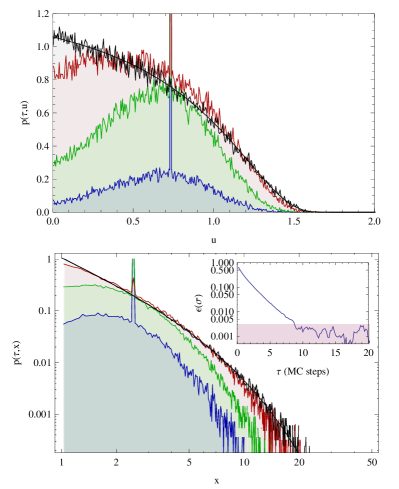
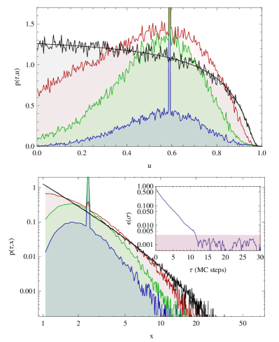
Using the same parameters as in the previous case, we depict if Fig. 7 the diffusion process at $0.1$, $0.5$ and $2$ MC steps for the cases $q=1.5$ and $q=2$ respectively, also sowing the convergence of the standard deviation. Systematically, the equilibrium densities do follow the predicted distributions found via the MaxEnt.

5 Conclusions

It is commonly believed that Jaynes’ MaxEnt (JM), used in conjunction with Shannon’s logarithmic information measure yields, after the concomitant variational process, only exponential probability distribution functions (PDF).

This fact was largely responsible for motivating statistical mechanics’ practitioners to look for other information measures tsallis . We have shown here that great versatility is gained by MaxEnt if some further, appropriate a priori “dynamical” knowledge is added to the JM-technique, a way of proceeding that entirely agrees with Jaynes’ philosophy jaynes ; katz . Indeed, we see that effective Hamiltonians for the process at hand are also a result of the MaxEnt technique.

The JM-procedure can in this fashion still keep Shannon’s measure while at the same yielding almost any functional form for the ensuing variational PDF, power laws in particular.

ACKNOWLEDGMENT: This work was partially supported by ANR DYNHELIUM (ANR-08-BLAN-0146-01) Toulouse, and the Projects FQM-2445 and FQM-207 of the Junta de Andalucía. AP acknowledges support from the Senior Grant CEI Bio-Tic GENIL-SPR.

References

- (1) E. T. Jaynes, (1957). Phys. Rev. 106, 620 (1957); 108, 171 (1957); IEEE Trans. Syst. Sci. & Cyb. 4, 227 (1968).
- (2) A. Katz, Principles of statistical mechanics: the information theory approach (W. H. Freeman, San Francisco, 1967).
- (3) M. E. J. Newman. Contemporary Physics, 46, 323 (2005).
- (4) S. K. Baek, S. Bernhardsson, P. Minnhagen, New J. Phys. 13, 043004 (2011).
- (5) H. Simon, Biometrika 42, 425 (1955).
- (6) B. Mandelbrot, Information and Control, 2, 90 (1959).
- (7) A. Hernando, D. Puigdomènech, D. Villuendas, C. Vesperinas, A. Plastino, Phys. Lett. A 374, 18 (2009).
- (8) A. Hernando, C. Vesperinas, A. Plastino, Phys. A 389, 490 (2010).
- (9) A. Hernando, D. Villuendas, C. Vesperinas, M. Abad, A. Plastino, Eur. Phys. J. B 76, 87 (2010).
- (10) F. Benford, (March 1938) Proceed. Am. Phil. Soc. 78, 551572 (1938).
- (11) Weisstein, Eric W., ”Benford’s Law” from MathWorld (http://mathworld.wolfram.com/BenfordsLaw.html).
- (12) M. Abramowitz, I. A. Stegun Eds., Handbook of Mathematical Functions with Formulas, Graphs, and Mathematical Tables Chapter 6.5 (Dover, New York, 1965).
- (13) C. Tsallis, J. Stat. Phys. 52 (1988) 479; Phys. Rev. E 58, 1442 (1998); L. Zunino et al., Physica A 388, 1985 (2009).