First SDO/AIA Observation of Solar Prominence Formation Following an Eruption: Magnetic Dips and Sustained Condensation and Drainage
Abstract
Imaging solar coronal condensation forming prominences was difficult in the past, a situation recently changed by Hinode and SDO. We present the first example observed with SDO/AIA, in which material gradually cools through multiple EUV channels in a transequatorial loop system that confines an earlier eruption. Nine hours later, this leads to eventual condensation at the dips of these loops, forming a moderate-size prominence of , to be compared to the characteristic mass of a CME. The prominence mass is not static but maintained by condensation at a high estimated rate of against a comparable, sustained drainage through numerous vertical downflow threads, such that 96% of the total condensation () is drained in approximately one day. The mass condensation and drainage rates temporally correlate with the total prominence mass. The downflow velocity has a narrow Gaussian distribution with a mean of , while the downward acceleration distribution has an exponential drop with a mean of , indicating a significant canceling of gravity, possibly by the Lorentz force. Our observations show that a macroscopic quiescent prominence is microscopically dynamic, involving the passage of a significant mass through it, maintained by a continual mass supply against a comparable mass drainage, which bears important implications for CME initiation mechanisms in which mass unloading is important.
Subject headings:
Sun: activity—Sun: corona—Sun: filaments, prominences1. Introduction
Solar prominences are over dense and cool material in the tenuous, hot corona (Tandberg-Hanssen, 1995; Martin, 1998; Labrosse et al., 2010; Mackay et al., 2010). Proposed mechanisms for prominence formation include: (1) chromospheric transport by siphon flows (Pikel’Ner, 1971; Engvold & Jensen, 1977), magnetic reconnection (Litvinenko & Martin, 1999; Wang, 1999), or magnetic flux emergence (Hu & Liu, 2000; Okamoto et al., 2009), and (2) coronal condensation due to a diversity of radiatively-driven thermal instabilities (Parker, 1953; Priest, 1982, p.277) occurring in current sheets (Smith & Priest, 1977; Titov et al., 1993) and coronal loops (Wu et al., 1990; Mok et al., 1990; Antiochos & Klimchuk, 1991; Choe & Lee, 1992; Karpen et al., 2003, 2005; Luna Bennasar et al., 2012).
Prominence formation by condensation was once questioned because a quiet, static corona is an inadequate mass source (Saito & Tandberg-Hanssen, 1973). This does not apply to the solar corona that is known to be dynamic with mass being continually replenished, say, by footpoint heating driving chromospheric evaporation (Karpen & Antiochos, 2008; Xia et al., 2011), by ubiquitous spicules (De Pontieu et al., 2011), or by thermal convection involving emerging magnetic bubbles (Berger et al., 2011).
Condensation was seen in the so-called “cloud prominences” (Engvold, 1976; Tandberg-Hanssen, 1995; Lin et al., 2006; Stenborg et al., 2008) or “coronal spiders” (Allen et al., 1998) with material streaming out along curved trajectories. It was also observed in cooling loops (Landi et al., 2009) and proposed to produce coronal rain (Schrijver, 2001; Müller et al., 2003). However, quantitative analysis of prominence condensation has been hampered by the high off-limb scattered light of ground-based instruments and limited spatial/temporal resolution or field of view (FOV) of previous space instruments.
This situation has changed with the launches of the Hinode and Solar Dynamics Observatory (SDO). SDO’s Atmospheric Imaging Assembly (AIA; Lemen et al., 2011) offers unprecedented capabilities with a full Sun FOV at 12 s cadence and resolution. Here we present a first AIA observation of prominence formation, involving magnetic dips and plasma condensing there to build up the prominence mass and balance sustained drainage. Observations of this kind may provide answers to three long-standing questions:
-
1.
How do condensation and drainage control the mass budget of a prominence?
-
2.
What are the favorable plasma and magnetic field conditions at the micro and macroscopic scales of a prominence?
-
3.
What is the relationship between prominences and other solar activities, such as CMEs and flares?
2. Observational Overview: Prominence Formation After Confined Eruption
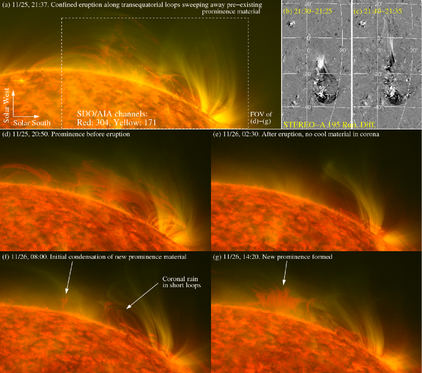
On 2010/11/25 at about 21:10 UT, a confined eruption is observed by SDO/AIA and STEREO A in NOAA active region (AR) 11126 (Figures 1(a)–(c); Animations 1(A) and 1(B)). Most of the pre-existing prominence material is swept away along transequatorial loops at and some lands on the other hemisphere.
At 2010/11/26 05:00 UT, the first sign of new, cool 304 Å material is observed at the dips in the active region loops and consequently slides downward along underlying loops as coronal rain (Figure 1(f); Animations 1(C)). Two hours later, a nearby condensation at greater rates leads to the formation of a new prominence (Figures 1(f) and (g)). After another day, the prominence gradually shrinks and eventually disappears behind the limb.
In this Letter, we focus on the condensation and mass drainage in the new prominence, leaving other interesting aspects of this event for future investigation.
3. Initial Condensation at Magnetic Dips in Transequatorial Loops
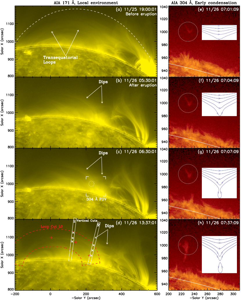
Let us first examine the magnetic environment. Prior to the eruption, there are transequatorial loops of various lengths, best seen at 171 Å in Figure 2(a) and Animation 1(A). The limb location of the event does not allow accurate determination of the magnetic configuration, but potential field extrapolations111http://sohowww.nascom.nasa.gov/sdb/packages/pfss/l1qsynop up to a week earlier indicate the persistence of such loops that connect the positive trailing polarity of AR 11126 in the south and the diffuse negative polarity in the north.222see magnetograms on 11/18 at http://www.solarmonitor.org
After the eruption, these loops fade and gradually reappear. Since 11/26 05:00 UT, one can can identify an apparent depression, likely formed in projection by shallow dips of numerous loops (Figure 2, left), where the initial condensation occurs shortly at 07:00 UT. The cool 304 Å material forms a “V”-shape (Figure 2, right), whose lower tip progressively drops and eventually drains down in a nearly vertical direction, suggesting magnetic reconnection (as sketched here) or cross-field slippage (Low et al. 2012b, in preparation).
4. Post-eruption Cooling in Transequatorial Loops
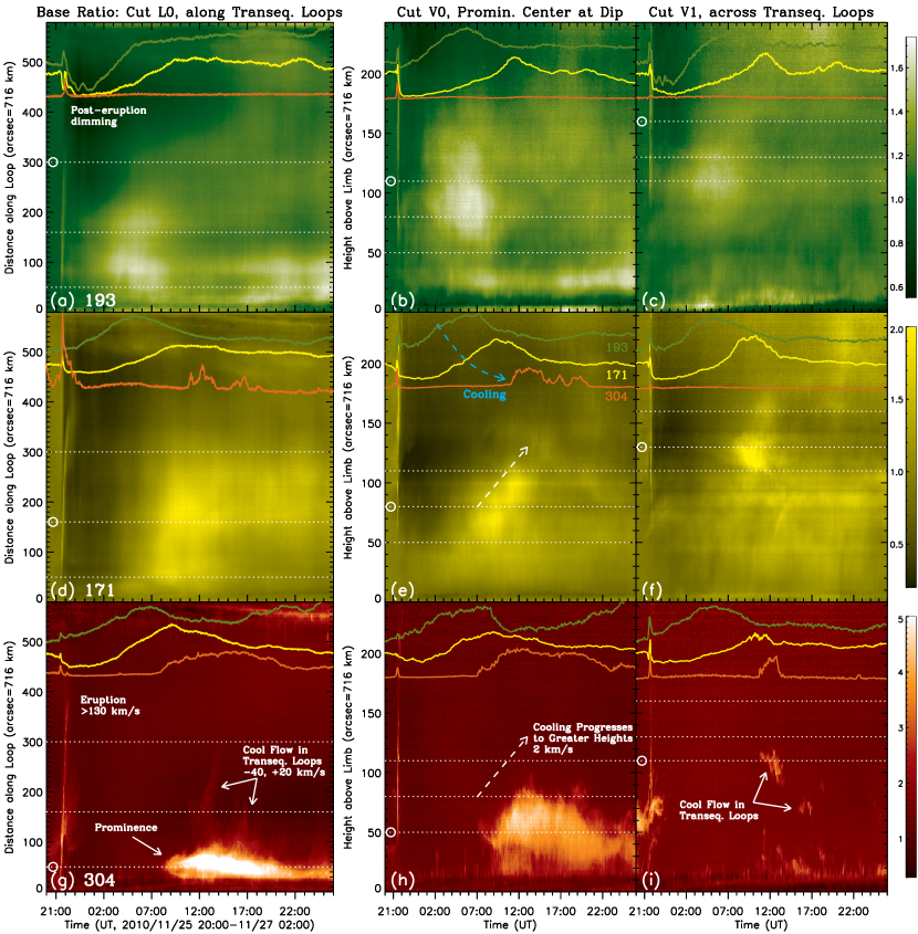
To track the cooling process and infer the origin of the prominence mass, we placed a () wide cut L0 along the transequatorial loops to the north of the dips and two vertical cuts of wide and tall from the limb across these loops at the lowest dip (V0) and further north (V1; Figure 2(d); cuts to the south of the dips yielded similar results). By averaging image pixels across each cut, we obtained space-time diagrams as shown in Figure 3 together with selected temporal profiles.
We find a general trend of successive brightening after the eruption at 193, 171, and then 304 Å, each delayed by 2–5 hours. This indicates gradual cooling across the characteristic temperatures at the response peaks of these broadband channels, from to and (Boerner et al., 2011). At 193 Å, the initial brightening likely results from mass being replenished after the eruption and/or cooling from even higher temperatures; the later darkening at 9:00 UT and heights – is primarily due to absorption by the cool prominence material.
Condensation of the 304 Å material occurs only at low altitudes () near the dips, while cooling from higher temperatures takes place almost throughout the entire transequatorial loop system involving a vast volume (Figure 3, left). This implies that these loops likely feed mass to the prominence forming at their dips that, partly because of the stretched and possibly sheared magnetic field lines (say, near a polarity inversion line) and thus reduced field-aligned thermal conduction, may facilitate further cooling and condensation (Low et al. 2012a, in preparation). We detected no systematic cooling flow in the loops though, possibly due to the insensitivity of AIA (passband imager) to subtle flows without distinct mass blobs, except for occasional brief downflows and upflows of 304 Å material (Figures 3(g)). The 9 hr elapsed from the eruption to the initial condensation is on the same order of magnitude as the condensation timescales in thermal nonequilibrium simulations (Karpen et al., 2005).
Condensation at 304 Å occurs first at a height of and progresses toward higher loops at (, the projected speed of the solar rotation there), with a similar trend at 171 Å (Figures 3(e) and (h)). We speculate that those low-lying loops condense first because of their shorter lengths (Karpen & Antiochos, 2008) and/or their greater densities from gravitational stratification (as radiative loss ).
5. Mass Budget of Condensation and Drainage
In this prominence, we find no sign of rising bubbles (Berger et al., 2008, 2010, 2011) that can contribute to the prominence mass. If we further neglect other possible mass sources, the interplay between the mass condensation rate and downflow rate would determine the prominence mass change rate
| (1) |
The condensation rate , which cannot be measured directly, can thus be inferred by measuring and independently, as described below in three steps.
5.1. Prominence Mass Budget
This prominence consists of numerous nearly vertical threads of typically (1.43 Mm) thick (see also Berger et al. 2008). The observed optically thick 304 Å emission originates from a layer known as the prominence-coronal transition region (PCTR) surrounding a denser, cooler H emitting core (e.g., Lin et al., 2005; Lin, 2011), later seen in Mauna Loa data (not shown). However, lacking sufficient H coverage of the event, we chose to use a typical PCTR electron density (Labrosse et al., 2010) and thus as a lower limit for the entire prominence. We also conservatively assumed that the observed threads do not overlap each other.
We selected a sector-shaped area to enclose the bulk of the prominence (see Figure 4(c)). The sector covers a height range of – above the limb and a latitude range of ( wide on its bottom edge). We then integrated the area occupied by the prominence material inside the sector for all pixels above a threshold selected at above background. We obtained a lower limit to the prominence mass
| (2) |
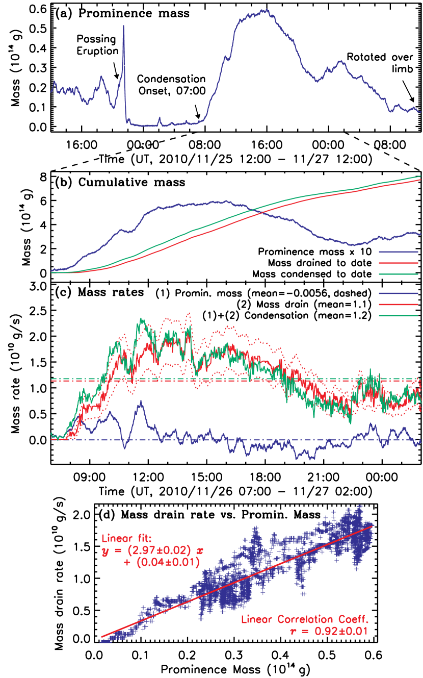
as shown in Figure 5(a). After the initial condensation, the prominence mass continues to increase and reaches the maximum at 16:01 UT,
which is on the same order of magnitude as that determined from coronal absorption for a prominence of similar size (Gilbert et al., 2005). Taking time derivative gives the mass change rate shown in Figure 5(c), which has a mean of and a maximum at 11:37 UT,
5.2. Mass drainage Rate
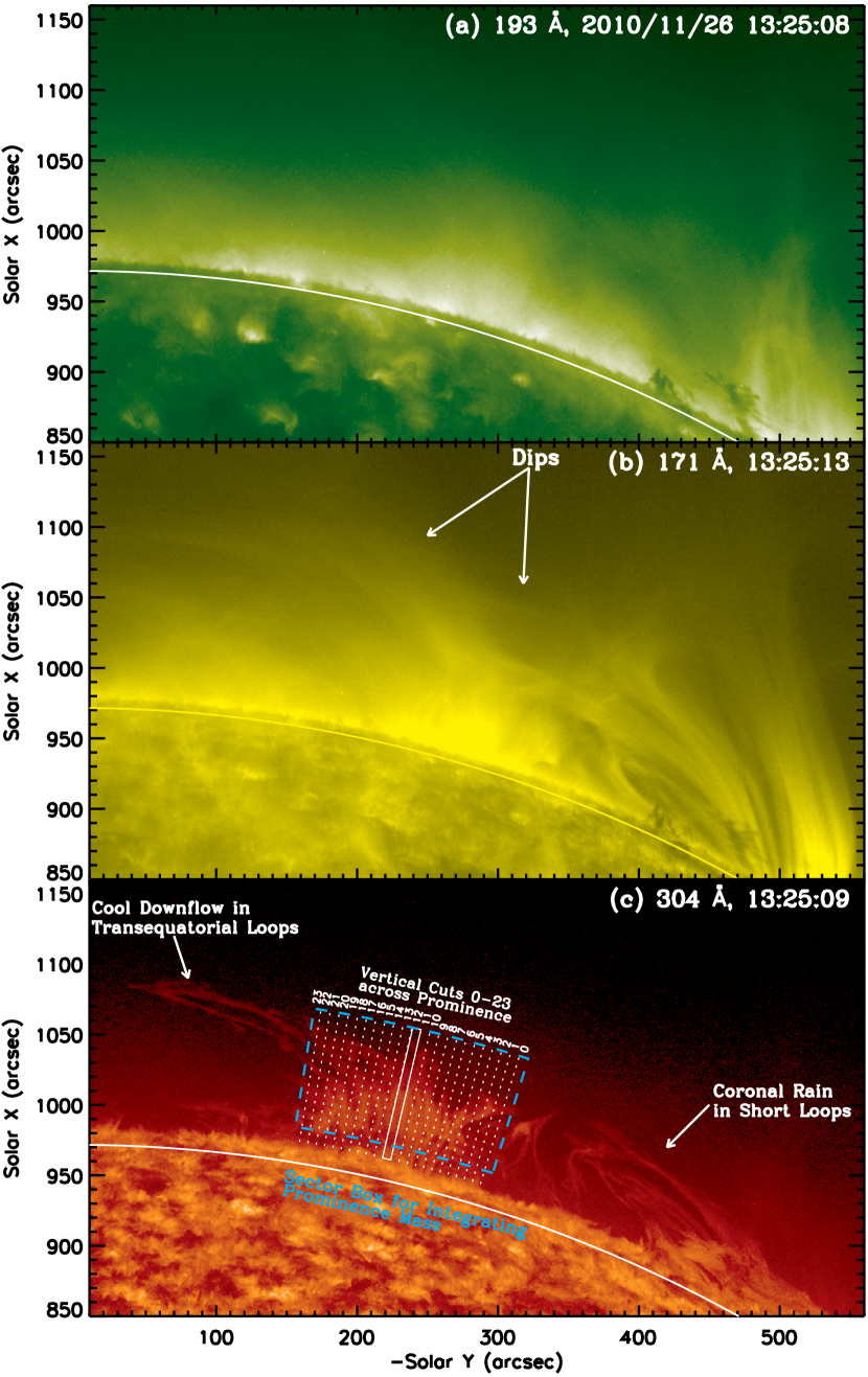

To estimate the drainage rate of mass that leaves the sector-shaped area, we need to obtain the downflow velocity at position on the bottom edge of the sector and at time , and then spatially integrate the mass flux crossing this edge. Here we assume that the warm PCTR and cool core of the prominence thread have the same downflow velocity (Labrosse et al., 2010). To measure , we divided the sector into 24 vertical cuts of wide333The width of the vertical cuts was chosen to be as small as possible and yet wide enough to enclose most of the prominence threads that are close to but not exactly vertical. that start at above the limb to avoid spicules and discretize the bottom sector edge into distance bins (), as shown in Figure 4(c). For each cut, we obtained a space-time diagram for a 19 hr duration from 11/26 07:00 to 11/27 02:00 UT.
As an example, the space-time diagram (Figures 4(d) and (e)) of cut #12 located near the middle of the prominence shows numerous, episodic downward curved trajectories. Each trajectory tracks the height of a blob of mass with time as it descends within the vertical cut. The descent covers a height range of several tens of arcseconds and lasts for a few minutes to half an hour. We fitted each well-defined trajectory with a parabolic function, as shown in Figure 4(d), and determined the average acceleration and velocity at the reference height (horizontal dashed line) of the bottom edge of the sector. We exhaustively repeated such fits throughout the space-time diagram, only skipping an adjacent trajectory of a similar slope within any 10 minutes interval. The resulting fits are overlaid in Figure 4(e), and the fitted velocities and accelerations are shown in Figures 4(f) and (g). Finally, we linearly interpolated the fitted velocities in time and obtained covering the full duration.
We applied this procedure to all vertical cuts across the prominence and obtained a statistically significant sample of 874 parabolic downflow trajectories. As shown in Figure 4(h), the fitted velocities have a narrow Gaussian distribution, with a mean and median of , mode of , and standard deviation of . In contrast, the accelerations (Figure 4(i)) have an exponential distribution , with a mean of , a standard deviation of , and a small mode of , where is the solar surface gravitational constant.
After obtaining the downflow velocity at all cuts, next we need the knowledge of the spatial width and temporal duration of each downflow stream. For the former, we assumed that within each wide cut, no more than one vertical thread (typical width ) undergoes downflow at any moment, giving an effective filing factor of . For the latter, we defined a switch function that describes whether downflow occurs () or not () at the th cut and time , depending on whether or not the emission intensity (e.g., Figure 4(d)) in the corresponding space-time diagram at height is above the pre-event background.
Finally, summing over all vertical cuts (as spatial integration) yields the mass drainage rate:
| (3) |
where is the cross-sectional area of the thread. As shown in Figure 5(c), it has a mean
and a maximum
at 11/26 14:08 UT. Integrating over time yields the accumulative mass drained to date , as shown in Figure 5(b). At the end of the 19 hr duration, it reaches
which is times the maximum prominence mass .
5.3. Mass Condensation Rate
The mass conservation equation (1) then gives the condensation rate
| (4) |
as shown in Figure 5(c). It closely follows the mass drainage rate , which dominates over the prominence mass change by about an order of magnitude. The condensation rate has a similar mean
and maximum
at 11/26 11:37 UT. The cumulative mass condensed in 19 hr is
about the same as the mass drained to date.
We find two episodes of rapid condensation and mass drainage, starting at 11/26 07:00 and 22:00 UT, which coincide with the variations of the prominence mass (Figure 5(b)). In fact, the drainage rate is positively correlated with the total prominence mass, with a linear correlation coefficient of (Figure 5(d)).
6. Summary and Discussion
We have presented new evidence of coronal condensation that leads to prominence formation at magnetic dips after a confined eruption. Our major findings and their implications are as follows.
-
1.
The estimated average mass condensation rate in the prominence is , giving an accumulative mass of in 19 hr. Most (96%) of this mass, an order of magnitude more than the instantaneous total mass of the prominence, is drained as vertical threads. In other words, a macroscopically quiescent prominence is a microscopically dynamic object, with a total mass determined by the delicate balance between a significant mass supply and a drainage by downflows. This was suggested long ago (e.g., Priest & Smith, 1979; Tandberg-Hanssen, 1995), but to the best of our knowledge, our observations provide the first quantitative evidence in terms of the prominence mass budget.
-
2.
The mass condensation and drainage rates are very close and linearly correlated with the total prominence mass. Thus, the more material the prominence has, the more mass it is capable of draining. Theoretical considerations of energy balance by Low et al. (2012b, in preparation) indicates that the total mass is a critical parameter that determines how fast condensation takes place.
-
3.
The prominence downflows are much slower than free fall, with an average acceleration of , similar to that found by Chae (2010). This shows that gravity in the prominence is countered significantly, possibly by an upward Lorentz force (e.g., Low & Petrie, 2005; van Ballegooijen & Cranmer, 2010) from the horizontal component of the magnetic field, as indicated by polarimetric measurements (Casini et al., 2003), or by transverse wave generated pressure as originally suggested for braking coronal rain (Antolin & Verwichte, 2011).
-
4.
After hours of cooling from throughout almost the entire transequatorial loop system that confined the early eruption, the initial prominence condensation () occurs at the loop dips and consequently progresses toward greater heights. This suggests that these large-scale loops may function like a funnel with a vast collecting volume that feeds mass to the prominence, and the dips likely provide favorable conditions for further cooling and condensation (cf., Karpen et al., 2001).
- 5.
-
6.
We propose that the passage of mass on the order of /day, comparable to a CME mass, could be a general property of prominences exhibiting active drainage. If the “magneto-thermal convection” suggested by Berger et al. (2011) in prominence-cavity structures also involves the drainage of such a large mass, its weight is energetically significant for holding a magnetic flux rope in the cavity until it erupts into a CME (Low, 2001; Zhang & Low, 2005).
This study and future observations of coronal condensation may provide further insights into prominences as an MHD phenomenon, with answers to the long-standing questions noted in the Introduction.
References
- Allen et al. (1998) Allen, U. A., Bagenal, F., & Hundhausen, A. J. 1998, in Astronomical Society of the Pacific Conference Series, Vol. 150, IAU Colloq. 167: New Perspectives on Solar Prominences, ed. D. F. Webb, B. Schmieder, & D. M. Rust, 290
- Antiochos & Klimchuk (1991) Antiochos, S. K. & Klimchuk, J. A. 1991, ApJ, 378, 372
- Antolin & Verwichte (2011) Antolin, P. & Verwichte, E. 2011, ApJ, 736, 121
- Berger et al. (2011) Berger, T., et al. 2011, Nature, 472, 197
- Berger et al. (2008) Berger, T. E., et al. 2008, ApJ, 676, L89
- Berger et al. (2010) Berger, T. E., et al. 2010, ApJ, 716, 1288
- Boerner et al. (2011) Boerner, P., et al. 2011, Sol. Phys., 316
- Casini et al. (2003) Casini, R., López Ariste, A., Tomczyk, S., & Lites, B. W. 2003, ApJ, 598, L67
- Chae (2010) Chae, J. 2010, ApJ, 714, 618
- Choe & Lee (1992) Choe, G. S. & Lee, L. C. 1992, Sol. Phys., 138, 291
- De Pontieu et al. (2011) De Pontieu, B., McIntosh, S. W., Carlsson, M., Hansteen, V. H., Tarbell, T. D., Boerner, P., Martinez-Sykora, J., Schrijver, C. J., & Title, A. M. 2011, Science, 331, 55
- Engvold (1976) Engvold, O. 1976, Sol. Phys., 49, 283
- Engvold & Jensen (1977) Engvold, O. & Jensen, E. 1977, Sol. Phys., 52, 37
- Gilbert et al. (2005) Gilbert, H. R., Holzer, T. E., & MacQueen, R. M. 2005, ApJ, 618, 524
- Hu & Liu (2000) Hu, Y. Q. & Liu, W. 2000, ApJ, 540, 1119
- Karpen & Antiochos (2008) Karpen, J. T. & Antiochos, S. K. 2008, ApJ, 676, 658
- Karpen et al. (2001) Karpen, J. T., Antiochos, S. K., Hohensee, M., Klimchuk, J. A., & MacNeice, P. J. 2001, ApJ, 553, L85
- Karpen et al. (2003) Karpen, J. T., Antiochos, S. K., Klimchuk, J. A., & MacNeice, P. J. 2003, ApJ, 593, 1187
- Karpen et al. (2005) Karpen, J. T., Tanner, S. E. M., Antiochos, S. K., & DeVore, C. R. 2005, ApJ, 635, 1319
- Labrosse et al. (2010) Labrosse, N., Heinzel, P., Vial, J.-C., Kucera, T., Parenti, S., Gunár, S., Schmieder, B., & Kilper, G. 2010, Space Sci. Rev., 151, 243
- Landi et al. (2009) Landi, E., Miralles, M. P., Curdt, W., & Hara, H. 2009, ApJ, 695, 221
- Lemen et al. (2011) Lemen, J. R., et al. 2011, Sol. Phys., 106
- Lin (2011) Lin, Y. 2011, Space Sci. Rev., 158, 237
- Lin et al. (2005) Lin, Y., Engvold, O., Rouppe van der Voort, L., Wiik, J. E., & Berger, T. E. 2005, Sol. Phys., 226, 239
- Lin et al. (2006) Lin, Y., Martin, S. F., & Engvold, O. 2006, in Bulletin of the American Astronomical Society, Vol. 38, AAS/Solar Physics Division Meeting #37, 219
- Litvinenko & Martin (1999) Litvinenko, Y. E. & Martin, S. F. 1999, Sol. Phys., 190, 45
- Low (2001) Low, B. C. 2001, J. Geophys. Res., 106, 25141
- Low & Petrie (2005) Low, B. C. & Petrie, G. J. D. 2005, ApJ, 626, 551
- Luna Bennasar et al. (2012) Luna Bennasar, M., Karpen, J., & DeVore, C. R. 2012, ApJ, in press
- Mackay et al. (2010) Mackay, D. H., Karpen, J. T., Ballester, J. L., Schmieder, B., & Aulanier, G. 2010, Space Sci. Rev., 151, 333
- Martin (1998) Martin, S. F. 1998, Sol. Phys., 182, 107
- Mok et al. (1990) Mok, Y., Drake, J. F., Schnack, D. D., & van Hoven, G. 1990, ApJ, 359, 228
- Müller et al. (2003) Müller, D. A. N., Hansteen, V. H., & Peter, H. 2003, A&A, 411, 605
- Okamoto et al. (2009) Okamoto, T. J., Tsuneta, S., Lites, B. W., Kubo, M., Yokoyama, T., Berger, T. E., Ichimoto, K., Katsukawa, Y., Nagata, S., Shibata, K., Shimizu, T., Shine, R. A., Suematsu, Y., Tarbell, T. D., & Title, A. M. 2009, ApJ, 697, 913
- Parker (1953) Parker, E. N. 1953, ApJ, 117, 431
- Pikel’Ner (1971) Pikel’Ner, S. B. 1971, Sol. Phys., 17, 44
- Priest (1982) Priest, E. R. 1982, Solar magneto-hydrodynamics (Dordrecht, Holland; Boston: D. Reidel Pub. Co.; Hingham,)
- Priest & Smith (1979) Priest, E. R. & Smith, E. A. 1979, Sol. Phys., 64, 267
- Saito & Tandberg-Hanssen (1973) Saito, K. & Tandberg-Hanssen, E. 1973, Sol. Phys., 31, 105
- Schrijver (2001) Schrijver, C. J. 2001, Sol. Phys., 198, 325
- Smith & Priest (1977) Smith, E. A. & Priest, E. R. 1977, Sol. Phys., 53, 25
- Stenborg et al. (2008) Stenborg, G., Vourlidas, A., & Howard, R. A. 2008, ApJ, 674, 1201
- Tandberg-Hanssen (1995) Tandberg-Hanssen, E. 1995, The nature of solar prominences (Dordrecht; Boston: Kluwer)
- Titov et al. (1993) Titov, V. S., Priest, E. R., & Demoulin, P. 1993, A&A, 276, 564
- van Ballegooijen & Cranmer (2010) van Ballegooijen, A. A. & Cranmer, S. R. 2010, ApJ, 711, 164
- Wang et al. (2007) Wang, J., Zhang, Y., Zhou, G., Harra, L. K., Williams, D. R., & Jiang, Y. 2007, Sol. Phys., 244, 75
- Wang (1999) Wang, Y.-M. 1999, ApJ, 520, L71
- Wu et al. (1990) Wu, S. T., Bao, J. J., An, C. H., & Tandberg-Hanssen, E. 1990, Sol. Phys., 125, 277
- Xia et al. (2011) Xia, C., Chen, P. F., Keppens, R., & van Marle, A. J. 2011, ApJ, 737, 27
- Zhang & Low (2005) Zhang, M. & Low, B. C. 2005, ARA&A, 43, 103