Large Magellanic Cloud Cepheids
in the ASAS data

P. K a r c z m a r e k¹, W. A. D z i e m b o w s k i^2,3, P. L e n z³, P. P i e t r u k o w i c z² and G. P o j m a ń s k i^{2 1} Nicolaus Copernicus University, ul. Gagarina 11, 87-100 Toruń, Poland
e-mail: karczmarek@astri.uni.torun.pl
² Warsaw University Observatory, Al. Ujazdowskie 4, 00-478 Warsaw, Poland
³ Copernicus Astronomical Center, ul. Bartycka 18, 00-716 Warsaw, Poland

A catalog of Cepheids in the Large Magellanic Cloud (LMC) from the ASAS project is presented. It contains data on 65 fundamental mode pulsators with periods longer than about 8 days. The period-luminosity (PL) relation in the $V$-band does not significantly differ from the relation determined by Soszyński et al. (2008) from the OGLE data extended toward longer periods but with much larger spread. For objects with periods longer than 40 d there is an evidence for a shallower PL relation. The rates of long-term period variations significant at $3\sigma$ level are found only for 7 objects. The rates for 25 objects determined with the $1\sigma$ significance are confronted with the values derived from stellar evolution models. The models from various sources yield discrepant predictions. Over the whole data range, a good agreement with measurements is found for certain models but not from the same source. Stars: evolution - Stars: Cepheids - Large Magellanic Cloud

1 Introduction

Crossing of the Cepheid Instability Strip is a short but important phase of massive stars evolution. Objects in this phase reveal periods of radial pulsation, which are valuable observables. The period-luminosity (PL) relation for Cepheids for nearly a century plays a crucial role in the cosmic distance ladder. A newer application of Cepheids is probing massive star evolution through measurements of the rates of period changes (see, e.g., Pietrukowicz 2001, Turner et al. 2006).

Bird et al. (2009) emphasize exceptional importance of long period objects, which they name Ultra Long Period (ULP) Cepheids, in both applications. Being bright, these objects are seen in distant galaxies, however the shape of the upper part of the PL relation is not yet well-established.

Open questions in the theory of massive stars concern, in particular, the rate of mass loss and the extent of mixing beyond the edge of convective core. There are related uncertainties in calculations of evolutionary tracks in the H-R diagram and life times in various phases in particular within the Cepheid instability strip. Here we find considerable differences between results presented by various authors (e.g., Schaerer et al. 1993, Fagotto et al. 1994, Alibert et al. 1999, Bono et al. 2000, Pietrinferni et al. 2006).

Long period Cepheids in both Magellanic Clouds are being monitored for nearly 10 years within the ASAS project (Pojmański 2002). A part of the ASAS data has been already employed in searches for period changes in a combination with Harvard data by Pietrukowicz (2001). The long-time data give us a chance to determine the rates of period change on the basis of the ASAS data alone by means of direct fitting of measurements. This will be done in the present paper, which is devoted exclusively to the object located in the LMC.

An extensive study of Cepheid period changes in this galaxy, based on the OGLE and MACHO data, was presented by Poleski (2008) but it was limited to objects with period below 40 days. The range of periods in the ASAS sample, which in contrast to that of the OGLE is limited from the bottom, is from 8 to 133 days. There is an overlap enabling a comparison of the results but also an extension to the interesting ULP range.

In the next section, we present an updated catalog of the LMC Cepheid in the ASAS data. Section 3 is devoted to the PL relation based on these data. In Section 4, we present our determination of period changes and confront them with values calculated for stellar models.

Figure 1: LMC Cepheids located inside the circle-shaped area with $r=11^{\circ}$ from the optical center of the LMC at RA = $5^{h}19^{m}$, Dec = -$69^{\circ}27^{\prime}$ (J2000.0 coordinates) (45^∘ angled cross in the middle). Pluses indicate objects classified in ASAS as DCEP-FU, open circles show objects originally classified as Miscellaneous or RRab stars.

2 Inventory of the LMC Cepheids in the ASAS data

In the ASAS catalog of fundamental mode Cepheids (available in the internet), we selected objects located within a radius of 11^∘ from the optical center of the Large Magellanic Cloud (Fig. 1), which is located at RA = $5^{h}19^{m}$, Dec = -$69^{\circ}27^{\prime}$ in J2000.0 coordinates (Subramaniam 2003).

In the specified area, we found 73 stars classified as Cepheids. After a careful inspection of the light curves, we rejected 5 objects. Another 7 objects were excluded for their distant positions in the PL plane from the classical PL relation for Cepheids. Then we looked for objects located in the same area in the sky with whose original ASAS classification was either Miscellaneous or RRab stars but classification as a fundamental mode Cepheid was given as an alternative. We added 4 objects to our list of Cepheids as they fulfilled the criteria of light curve shape and location in the PL plane.

The 65 objects which passed our selection criteria cover the period range from 8 to 133 days. Stars with shorter periods are too faint to be observed by ASAS. Only $V$-band data were employed in this paper. We have attempted to use the $I$-band data, however the number of measurements in this band was insufficient to determine meaningful light curves. Figs. 2 and 3 present the $V$-band light curves of all objects except of ASAS 050601-6906.3, which is very similar to ASAS 050346-6852.6. The light curves are repeated twice for clarity. We see no trend in the behavior of amplitudes with period. The lack of an apparent trend may be in part blamed to blending. Although the amplitudes of the stars are uncertain, it does not affect the accuracy of period changes which are of our main interest in this paper.

Selected data on all confirmed Cepheids are listed in Table 1. Data in consecutive columns of the table give: ASAS star identification, OGLE and/or Harvard identifications (if available), mean $V$ magnitude, amplitude, period, dimensionless rate of period change, signal-to-noise ratio (S/N) for the rate, and number of data points.

Figure 2: $V$-band light curves of the ASAS Cepheids with periods in the range of 8-24 days. In each graph top left number shows the logarithm of period in days and top right the ASAS ID of the star. The light curves are repeated twice for clarity.

Figure 3: The same as Fig. 2 but period range is 25-133 days.

Table 1: List of 65 ASAS Cepheids in the Large Magellanic Cloud

ASAS ID	OGLE/Harvard ID	$\langle V\rangle\pm\Delta V$	Amp.	$\log(P)$	$\dot{P}$	S/N	$N$
		[mag]	[mag]	[d]	$\times 10^{-6}$
050008-6827.0	HV883	12.18 $\pm$ 0.11	1.41	2.125	-48.1	0.62	764
051931-6841.2	HV2447	12.04 $\pm$ 0.06	0.67	2.075	24.0	0.46	1010
045541-6625.7	HV5497	11.90 $\pm$ 0.05	0.66	1.995	232.7	6.48	661
054347-6635.2	HV2827	12.28 $\pm$ 0.06	0.63	1.896	161.4	6.94	833
054451-6729.6	-	11.68 $\pm$ 0.05	0.47	1.871	-22.7	1.02	953
050716-6853.0	OGLE-LMC-CEP-0992	12.22 $\pm$ 0.06	0.47	1.724	-4.5	0.22	776
053122-7057.4	OGLE-LMC-CEP-2253/HV2622	12.88 $\pm$ 0.07	0.86	1.719	6.0	0.54	580
051354-6703.8	OGLE-LMC-CEP-1290/HV2369	12.68 $\pm$ 0.08	1.14	1.685	56.1	7.24	784
052508-6738.7	HV953	12.29 $\pm$ 0.06	1.08	1.682	11.3	2.09	1163
050648-7002.2	OGLE-LMC-CEP-0966/HV900	12.89 $\pm$ 0.08	1.09	1.676	80.9	6.90	606
045702-6759.7	OGLE-LMC-CEP-0461/HV877	13.38 $\pm$ 0.10	0.92	1.655	-15.3	0.95	582
050609-7115.4	OGLE-LMC-CEP-0943/HV2338	12.84 $\pm$ 0.08	1.22	1.625	32.1	4.64	615
045811-6957.0	OGLE-LMC-CEP-0512/HV2257	13.07 $\pm$ 0.09	1.35	1.596	-2.3	0.30	615
050920-7027.4	OGLE-LMC-CEP-1113/HV909	12.83 $\pm$ 0.08	1.09	1.575	-20.9	3.64	661
045805-6927.2	OGLE-LMC-CEP-0510/HV879	13.43 $\pm$ 0.10	1.28	1.566	3.1	0.39	551
050615-6640.8	OGLE-LMC-CEP-0945/HV2294	12.78 $\pm$ 0.07	1.27	1.563	1.1	0.26	657
045833-7020.8	OGLE-LMC-CEP-0528/HV881	13.14 $\pm$ 0.09	1.27	1.553	3.2	0.54	628
045423-7054.1	OGLE-LMC-CEP-0328/HV873	12.92 $\pm$ 0.07	1.23	1.537	-4.5	0.92	690
045941-6927.4	OGLE-LMC-CEP-0590/HV882	13.45 $\pm$ 0.11	1.32	1.502	1.5	0.23	588
050708-6853.3	OGLE-LMC-CEP-0986/HV899	13.54 $\pm$ 0.13	1.32	1.492	11.6	1.64	515
053550-6642.1	HV1002	13.06 $\pm$ 0.10	1.34	1.484	13.0	5.45	1196
050819-6846.7	OGLE-LMC-CEP-1058/HV904	13.08 $\pm$ 0.09	0.88	1.483	-2.9	0.45	780
045627-6922.9	OGLE-LMC-CEP-0434/HV875	12.75 $\pm$ 0.07	0.66	1.482	-13.0	1.56	661
045506-6728.6	OGLE-LMC-CEP-0367/HV872	13.52 $\pm$ 0.12	0.89	1.475	5.3	0.61	620
044537-7015.0	OGLE-LMC-CEP-0068/HV8036	13.62 $\pm$ 0.12	1.33	1.453	-2.7	0.61	823
052018-6756.8	OGLE-LMC-CEP-1632/HV934	14.09 $\pm$ 0.16	1.05	1.450	2.5	0.23	421
052655-6958.9	OGLE-LMC-CEP-2019/HV2540	13.41 $\pm$ 0.11	0.95	1.449	-3.0	0.37	515
050055-6638.2	OGLE-LMC-CEP-0654/HV225	13.17 $\pm$ 0.11	1.31	1.445	-4.8	1.07	600
051833-6712.9	HV929	13.87 $\pm$ 0.14	0.86	1.445	5.9	0.84	687
050720-7027.2	OGLE-LMC-CEP-0999/HV902	13.34 $\pm$ 0.10	1.33	1.421	1.7	0.48	603
053003-6556.1	HV12815	13.59 $\pm$ 0.12	1.03	1.417	3.1	0.86	1013
050349-6856.1	OGLE-LMC-CEP-0821/HV889	13.72 $\pm$ 0.13	1.02	1.412	-9.4	1.71	515
053537-6832.1	OGLE-LMC-CEP-2504/HV1003	13.33 $\pm$ 0.11	1.20	1.386	-1.3	0.48	947
045745-6542.5	HV6098	12.99 $\pm$ 0.07	0.88	1.385	2.1	0.75	625
053954-6750.2	OGLE-LMC-CEP-2832/HV1013	13.83 $\pm$ 0.14	0.95	1.383	-0.2	0.03	576
050308-6613.8	HV886	13.47 $\pm$ 0.12	1.41	1.380	4.0	1.25	582
052112-6903.1	OGLE-LMC-CEP-1677/HV938	13.64 $\pm$ 0.13	1.03	1.372	1.7	0.33	572
045751-6957.4	OGLE-LMC-CEP-0501/HV878	13.63 $\pm$ 0.12	1.42	1.367	2.5	0.71	512
053014-6926.3	OGLE-LMC-CEP-2176/HV984	13.43 $\pm$ 0.12	0.65	1.363	11.0	2.14	658
045713-6723.0	OGLE-LMC-CEP-0467/HV876	13.44 $\pm$ 0.13	1.16	1.356	1.5	0.33	506
044707-6917.7	OGLE-LMC-CEP-0079/HV1	14.05 $\pm$ 0.13	1.03	1.353	15.2	2.84	387
050346-6852.6	OGLE-LMC-CEP-0819/HV2291	13.76 $\pm$ 0.13	0.81	1.349	0.5	0.08	448
045004-6815.6	OGLE-LMC-CEP-0147/HV12446	13.44 $\pm$ 0.11	0.98	1.348	-1.3	0.35	627
050326-6909.0	OGLE-LMC-CEP-0801/HV2292	13.52 $\pm$ 0.13	1.01	1.328	-4.6	1.28	560
052429-7217.1	HV12804	14.02 $\pm$ 0.14	0.95	1.327	-10.7	2.00	297
050601-6906.3	-	14.10 $\pm$ 0.16	1.34	1.325	2.2	0.45	369
ASAS ID	OGLE/Harvard ID	$\langle V\rangle\pm\Delta V$	Amp.	$\log(P)$	$\dot{P}$	S/N	$N$
		[mag]	[mag]	[d]	$\times 10^{-6}$
044518-6916.6	OGLE-LMC-CEP-0063	13.43 $\pm$ 0.11	0.57	1.323	3.5	0.60	911
052056-6639.7	-	14.10 $\pm$ 0.17	0.93	1.316	-3.7	0.43	443
050154-6854.3	OGLE-LMC-CEP-0712/HV885	13.49 $\pm$ 0.11	1.02	1.316	-2.0	0.46	357
045247-6820.9	OGLE-LMC-CEP-0249/HV11	13.92 $\pm$ 0.13	0.93	1.303	2.7	0.74	419
050308-6913.4	OGLE-LMC-CEP-0787/HV2288	13.24 $\pm$ 0.09	0.50	1.244	0.0	0.01	580
051514-6549.1	HV2888	14.21 $\pm$ 0.15	1.13	1.243	-4.3	1.05	317
045836-7006.6	OGLE-LMC-CEP-0535/HV2261	13.75 $\pm$ 0.15	1.40	1.237	-0.1	0.03	523
052926-6614.4	HV2580	14.10 $\pm$ 0.17	0.98	1.228	0.5	0.17	634
052700-7138.6	OGLE-LMC-CEP-2023/HV2549	13.96 $\pm$ 0.14	1.10	1.210	3.2	1.34	420
053259-6643.5	HV2667	14.07 $\pm$ 0.16	1.11	1.210	5.8	2.61	651
045847-7003.7	OGLE-LMC-CEP-0545/HV2262	14.03 $\pm$ 0.16	0.93	1.200	3.0	0.69	379
050803-7157.6	HV1276	14.02 $\pm$ 0.15	1.09	1.194	1.9	0.70	379
045848-6719.0	OGLE-LMC-CEP-0546/HV2249	13.52 $\pm$ 0.12	0.70	1.182	-4.7	1.87	604
045751-6750.3	OGLE-LMC-CEP-0500/HV2244	13.82 $\pm$ 0.14	0.94	1.145	-1.4	0.43	360
052548-6721.2	HV955	13.95 $\pm$ 0.15	0.97	1.138	-0.7	0.31	543
050904-7021.9	OGLE-LMC-CEP-1100/HV2352	14.26 $\pm$ 0.14	0.88	1.135	3.5	1.08	262
054118-7211.9	OGLE-LMC-CEP-2922/HV12839	14.16 $\pm$ 0.14	0.91	1.106	2.6	1.04	297
050252-7142.1	HV12745	14.58 $\pm$ 0.18	1.21	1.088	-4.6	1.70	201
044324-6913.7	OGLE-LMC-CEP-0046/HV12717	14.18 $\pm$ 0.17	0.59	0.947	3.7	0.93	198

3 Period-luminosity relation

Figure 4: Period-luminosity relation for the ASAS Cepheids. The four objects added to ASAS are shown with the encircled symbols. The solid line corresponds to the least square fit (see Eq. (1)). The dashed line shows the same for the OGLE Cepheids (see Eq. (2)), as determined by Soszyński et al. (2008).

With the data given in Table 1, we constructed the PL diagram in $V$-band, which is shown in Fig. 4. Errors in period measurements are very small (within the symbols). The linear least squares fit yields

$$V_{\rm ASAS}=-2.366(\pm 0.166)\log P+16.784(\pm 0.239),\quad\sigma=0.31\rm~{}mag.$$ (1)

This may be compared with the PL relation for single-mode Cepheids determined by Soszyński et al. (2008) on the basis of the OGLE data

$$V_{\rm OGLE}=-2.762(\pm 0.022)\log P+17.530(\pm 0.015),\quad\sigma=0.23\rm~{}mag.$$ (2)

The lines corresponding to these two relations are shown in Fig. 4. The four added objects are well within 3$\sigma$ of the ASAS fit which was the argument for including them to the sample.

We may see that our relation is not in a significant conflict with the extension of the OGLE PL relation, which was based on the sample limited to $\log(P)<1.7$. The slopes differ by less than $3\sigma$. The scatter of the ASAS luminosities is much larger, which in part is due to much smaller size of our sample and in part due to blending. The shallower slope of the ASAS relation may result from statistical bias connected with different magnitude ranges in the two samples but it is well possible that the difference reflects a real nonlinearity of the PL relation. In fact, a significant flattening of this relation in the long period range has been suggested by Bird et al. (2009). For their sample of the ULP Cepheids, they find the slope $-1.09\pm 0.94$ with $\sigma$ = 0.40 mag. The lower period limit for these objects is $\log(P)=1.9$. Our sample contains only three objects above this limit. In the range extended down to $\log(P)>1.6$ we have 12 objects. For this sample the slope of $-1.95\pm 0.65$ with $\sigma$ =0.38 mag, which is not in contradiction with the assessment quoted by Bird et al..

4 Search for evolutionary period changes

Certainly most of long-period Cepheids are objects burning helium in their convective core. Measuring rate of period changes for these objects is important because the evolution is still not fully understood. The difficulties in modeling stars in this phase of stellar evolution were first discussed by Paczyński (1970). The problem was subsequently studied in great details by Lauternborn et al. (1971), whose results were described in a separate chapter of the Kippenhahn and Weigert (1990) monograph. Nonetheless, considerable and difficult to explain differences between evolutionary tracks calculated by different authors are present to these days. The crucial problem is the occurrence and extent of the blue loops in this phase of evolution. We still do not know which of stellar and/or modeling parameters play the role. Most recent models from BaSTI library (Pietrinferni et al. 2006) do not help in answering this question. Uncertainties in modeling are best reflected in the rate of stellar period changes.

Figure 5: Rates of period change for the whole ASAS sample of LMC Cepheids. The $1\sigma$ error bars represent uncertainty of the fit of measurements to Eq.(3).

4.1 The method and results

To conduct our investigation on period changes, a modified version of Period04 (Lenz and Breger 2005) was used. Fortunately, the observed period changes are small and do not harm the effectiveness of frequency detection by Fourier techniques. The formula used for least squares fitting, however, was modified to include a parabolic frequency change,

$$f(t)=A_{0}+\sum_{i=1}^{n}A_{i}\sin(2\pi(\gamma t^{2}+\nu_{i}t+\phi_{i})),$$ (3)

where $A_{0}$ is the zero point in amplitude, $n$ is the number of terms, $\gamma$ is the frequency change parameter and $A_{i}$, $\nu_{i}$, and $\phi_{i}$ are amplitude, frequency and phase of the term $i$. Nonlinear least squares fits require good initial parameters; otherwise, the algorithm may get trapped in a local minimum of the $\chi^{2}$ hypersurface. The discrete Fourier transform provides an initial guess for the frequencies and amplitudes. To obtain good initial values for the other parameters we used the following sequential approach: first we adopted the frequency as given by the Fourier routine, assumed $\gamma=0$ and improved only the amplitudes and phases by means of a least squares fit. Based on this solution we determined a better initial value for the frequency change parameter $\gamma$. The modified Period04 version computed $\chi^{2}$ for different test values of $\gamma$ ranging within a predefined interval from $-10^{-6}$ to $+10^{-6}$. The $\gamma$ value with the lowest $\chi^{2}$ was then used as initial value to compute the full least squares solution according to the formula given in Eq. (3).

To give an estimate for the confidence limits of the parameters, Period04 computed the parameter uncertainties as a byproduct of the least squares fit and, as a second independent option, through Monte Carlo simulations. Finally, the frequency change parameter, $\gamma$, was transformed to the period change $dP/dt$ as given $dP/dt=-2\gamma/\nu^{2}$, taking into account error propagation.

The fact that the period change can be determined for any Cepheid is undeniable advantage of this method. Unfortunately, as we may see in Fig. 5, in many cases uncertainties of the $dP/dt$ are huge. In the sample of 65 Cepheids only for 7 objects the measured rates are significant at the 3$\sigma$ level (S/N=3). For comparison with rates of evolutionary period changes calculated from stellar models we will use the values for 25 objects with S/N>1.

In Fig. 6 we compare uncertainties of the period change rates for all 65 objects as determined with Period04 code with the values based on Pilecki’s et al. (2007) approximate expression for the uncertainty of the period change rate,

$$\sigma_{\rm est}\approx\frac{12P^{2}_{\rm sin}}{N^{1/2}T^{2}}\frac{\sigma}{A},$$ (4)

which is valid in the case of a star with the sinusoidal light curve observed $N$ times, uniformly distributed over time $T$ with a photometric error $\sigma$, period of a sinusoid $P_{\rm sin}$ and full-amplitude $A$. We see a good correlation but $\sigma_{\rm P04}$ is 1.2 to 2 times greater than $\sigma_{\rm est}$.

Figure 6: Comparison of uncertainties computed with Period04 with those calculated with Eq. (4).

We should stress that the uncertainties may include not only the measurement errors but possibly also the effect of fast period variations arising from nonlinear effects in stellar pulsation. It is impossible to disentangle these two effects in individual cases. Poleski (2008), who studied period changes in the LMC Cepheids in the OGLE and MACHO data, found fast variation only in 18 percent of fundamental mode pulsators. Thus, it seems unlikely that such variations are main source of the large uncertainties.

For some of our objects, we could compare our rates of period change with the results published by Pietrukowicz (2001) and Poleski (2008). Pietrukowicz (2001) based his determination of period changes on differences between the ASAS and Harvard periods for 19 LMC Cepheids. The advantage of his approach is the long-time base but the use of period rather than phase data is the price. The comparison of the rates determined in this way with our values is shown in Fig. 7. The agreement is satisfactory. Only in one case the difference exceeds $2\sigma$.

Figure 7: Comparison of period rate changes determined in this work with the values obtained by Pietrukowicz (2001).

Figure 8 compares rates of period changes determined in the present work with the values obtained by Poleski (2008) for the OGLE data. In his determinations, he relied on the traditional O-C diagrams method and on Fourier parameter fitting, similar to ours. From his large sample, we used only rates for 7 overlapping objects with S/N>3. The agreement is again fairly good. In the two cases where larger differences between the results are seen, the uncertainty in the OGLE rates might have been underestimated (Poleski, priv. com.).

As all our predecessors, we assume that the linear period changes which we determined for the the selected 25 Cepheids yield a realistic assessment of period changes resulting solely from evolutionary changes on stellar parameters. It should be stressed, however, that it is an assumption because nonlinear effects in stellar pulsations are not yet understood well enough to exclude pulsational origin of very slow period changes. We now proceed to compare the rates we determined with the values calculated for different sequences of stellar models. The comparison is done in the $(\log P,{\rm d}P/{\rm d}t)$ plane. Certainly, with the use of additional data, the comparison would be more constraining but ASAS do not provide any with an adequate precision.

Figure 8: Comparison of period rate changes determined in this work with the values obtained by Poleski (2008).

4.2 Comparison with predictions from stellar models

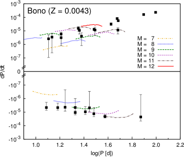
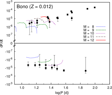
Figure 9: Comparison of the measured rates of period change with rates calculated from Bono et al. (2000) models at two indicated metallicity parameters, $Z$, and indicated initial masses, $M$, in solar units. The third crossing may be distinguished from the first crossing by the lower rates at specified periods and the longer periods at specified mass. At $M=12M_{\odot}$ there is only one crossing.

In Fig. 9 rates of period changes determined for the ASAS sample of LMC Cepheid are compared with the calculated values obtained from Bono et al. (2000) models at two metal abundance parameters, $Z$, around the value of $Z=0.008$, which is typically assumed for the young LMC objects. We should note that the positive measured rates are between those calculated for the first and third crossing of the instability strip for both values of $Z$. Since the relative chance for capturing an object during the first crossing is expected much lower than during the third crossing, this may suggest that the calculated rate for the third crossing is somewhat low. As for the negative rates, the agreement with the calculated rates at $Z=0.0043$ is good but at $Z=0.012$ the calculated rates are again somewhat lower than measured. Pietrukowicz (2001), who also compared his determinations with rates inferred from Bono et al. models, concludes that this comparison revealed "a crude agreement". Unfortunately, the calculated numbers cover only the short period part of our sample.

To cover the whole range of periods, we used data from evolutionary tracks calculated by Fagotto et al. (1994) and Schaerer et al. (1993). The data do not include pulsation periods and, thus, we calculated them with our code for envelope models with the surface parameters taken from the tracks. The models are rather scarce in time, therefore we determined only ages and periods interpolated at the ends of the instability strip crossings. We approximated the values of effective temperatures at the blue and red ends of the instability strip with the linear relations, $\log T_{\rm eff,blue}=3.803-0.045[\log(L/L_{\odot})-3]$ and $\log T_{\rm eff,red}=3.740-0.060[\log(L/L_{\odot})-3]$, respectively, which are based on nonlinear pulsation models calculated by Smolec and Moskalik (2008). For these models, only one rate for each crossing is given in Fig. 10. The bars at a given rate extend over the period ranges for the corresponding instability strips.

The models were calculated with the same metal abundance parameter, $Z=0.008$. The initial He abundance adopted by Fagotto et al. models is by about 5 percent lower than by Schaerer et al. There are differences in the adopted mass loss rate and overshooting from convective cores. In a consequence the period ranges in the corresponding instability strips at the same mass are somewhat shorter in the former models. The rates of period decrease during the second crossing are similar and, especially in the short period range, much lower than we determined from the ASAS data. Let us recall that in this range the measured rates agree quite well with calculated with Bono et al. (2000) models. As we may see in Fig. 10, the rates of period increase calculated by Fagotto et al. and Schaerer et al. differ quite a lot. In the first case, the mean rate of period change is significantly lower during the third than the first crossing, except at $M=15M_{\odot}$, when the opposite is true. In the second case, the rates are very similar during these two crossing except at $M=15M_{\odot}$, when the rate during the third crossing is significantly lower. Our rates of period increase are satisfactorily reproduced with Schaerer et al. (1993) models at $\log P\leq 1.7$ but at longer periods Fagotto et al. (1994) models do much better. The measured rates of period decrease are somewhat faster than predicted by models from both sources.

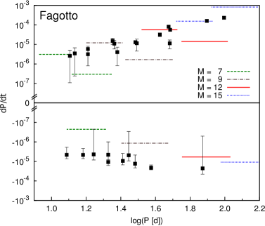
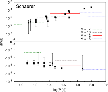
Figure 10: Comparison of the measured rates of period change with rates calculated from Fagotto et al. (1994) and Schaerer et al. (1993) models at indicated initial masses, $M$, in solar units.

5 Conclusions

We updated the list of Large Magellanic Cloud Cepheids in the ASAS sample and recalculated their pulsation characteristics and mean magnitudes in the $V$-band. The current list, which is given in Section 2, contains 65 confirmed objects covering the period range from 8 to 133 days. With these data, we determined the linear PL relation.

Within its large uncertainty, the PL relation from ASAS data does not significantly differ from that determined based on the OGLE data (Soszyński et al. 2008) linearly extended towards longer periods. For the sample of 12 objects with period longer than 40 days we found a flatter dependance which agrees with that determined by Bird et al. (2009). The large uncertainty is presumably caused mainly by reddening. Unfortunately the scarce data in the $I$-band did not allow to determine the reddening-free relation employing the Wesenheit index. Hopefully it will be possible in the future and this will help in the interpretation of period changes.

We tried to determine the rates of evolutionary period changes for all 65 objects. However, only for 25 we derived values significant at 1$\sigma$ level. The uncertainty may arise from measurement errors but it may arise also from non-evolutionary period variations. We argued that the first cause is dominant. Both, negative and positive rates were found. For some of the objects, we could compare the rates with earlier determinations and we find a reasonable agreement.

The derived rates were also compared with the values calculated for stellar models. We noted that the models from different sources yield very different values at similar parameters. The negative rates in the short period range are well reproduced by models in the second crossing phase calculated by Bono et al. (2000). The positive rates in the short-period range are in good agreement with Schaerer et al. (1993) models but in the long-period range the agreement with Fagotto et al. (1994) models is much better. We thank Radek Poleski for helpful information and remarks and Igor Soszyński (the referee) for his constructive comments. PK gratefully acknowledges support from Nicolaus Copernicus Center during her stays in 2010 and 2011. PP is supported from funding to the OGLE project from the European Research Council under the European Community^′s Seventh Framework Programme (FP7/2007-2013)/ERC grant agreement no. 246678, and by the grant No. IP2010 031570 financed by the Polish Ministry of Sciences and Higher Education under Iuventus Plus programme. Part of the research presented in this was supported by the Polish MNiSW grant number N N203 379636.

References

- \refitemAlibert, Y., Baraffe, I., Hauschildt, P., and Allard, F.1999Å344551 \refitemBird, J.C., Stanek, K. Z., and Prieto, J.L.2009\AJ695874 \refitemBono, G., Caputo, F., Cassisi, S., Marconi, M., Piersanti, L., and Tornambe, A.2000\ApJ543955 \refitemFagotto, F., Bressan, A., Bertelli, G., and Chiosi, C.1994Å10529 \refitemKippenhahn, R., and Weigert, A.1990Stellar Structure and EvolutionXVISpringer-Verlag Berlin Heidelberg New York \refitemLauterborn, D., Refsdal, S., and Weigert, A.1971Å1097 \refitemLenz, P., and Breger, M.2005Commun. Astroseismology14653 \refitemPaczyński, B.1970\Acta20195 \refitemPietrinferni, A., Cassisi, S., Salaris, M., and Castelli, F.2006\AJ642797 \refitemPietrukowicz, P.2001\Acta51247 \refitemPilecki, B., Fabrycky, D., and Poleski, R.2007\MNRAS378757 \refitemPojmański, G.2002\Acta52397 \refitemPoleski, R.2008\Acta58313 \refitemSchaerer, D., Meynet, G., Maeder, A., and Schaller, G.1993Å98523 \refitemSmolec, R., and Moskalik, P.2008Å58193 \refitemSoszyński, I., Poleski, R., Udalski, A., Kubiak, M., Szymański, M., Pietrzyński, I., Wyrzykowski, Ł., Szewczyk, O., and Ulaczyk, K.2008\Acta58163 \refitemSubramaniam, A.2003ApJL59819 \refitemTurner, D. G., and Abdel-Latif, M., A.-S.2006\PASP118410