The Self-Calibrating Hubble Diagram

Abstract

As an increasing number of well measured type Ia supernovae (SNe Ia) become available, the statistical uncertainty on $w$ has been reduced to the same size as the systematic uncertainty. The statistical error will decrease further in the near future, and hence the improvement of systematic uncertainties needs to be addressed, if further progress is to be made. We study how uncertainties in the primary reference spectrum – which are a main contribution to the systematic uncertainty budget – affect the measurement of the Dark Energy equation of state parameter $w$ from SNe Ia. The increasing number of SN observations can be used to reduce the uncertainties by including perturbations of the reference spectrum as nuisance parameters in a cosmology fit, thus “self-calibrating” the Hubble diagram.
We employ this method to real SNe data for the first time and find the perturbations of the reference spectrum consistent with zero at the 1%-level. For future surveys we estimate that $\sim\!3500$ SNe will be required for our method to outperform the standard method of deriving the cosmological parameters.

1 Introduction

Since the discovery of the accelerated expansion of the universe [1, 2, 3, 4, 5] type Ia supernovae (SNe Ia) have proven an excellent tool for probing the Dark Energy equation of state (EOS). Over the last decade the sensitivity of the measurements has increased due to the inclusion of larger, better calibrated data sets [6, 7, 8, 9, 10, 11, 12, 13]. By now, the statistical uncertainties in the measurement of the EOS match the size of the systematic ones (see e.g. [12, 14]). With an expected increase in the number of SNe that will be available from future surveys, the statistical errors will decrease fast, hitting the “systematic error wall” – if the systematic uncertainties cannot be reduced.

Measuring cosmological parameters from SNe Ia relies on comparing the luminosity distances of distant SNe with those of nearby ones. While the measurements of high-redshift SNe rely on redder bands (e.g. $r$, $i$ and $z$), small/intermediate distances require bluer bands (e.g. $u$ and $g$) as well [15]. Therefore the chromatic error in the flux calibration is a main contribution to the systematic uncertainties of cosmological parameters. Two main sources for chromatic uncertainties are the systematic errors for the zero-point determination for any given survey and the measurement of the fundamental flux standard that all surveys use to compare their measurements.

For the effect of zero-point uncertainties, it was shown [12, 14] that a 1% shift in the zero-point for a given high-redshift survey causes a variation of $\sim\!0.04$ in the dark energy equation of state parameter $w$.

With regard to the error for the fundamental flux standard, the generic calibration procedure can be summarized as follows: One or more fundamental spectroscopic standard stars, for which the spectral energy distributions (SEDs) are assumed to be known from careful modelling, serve as a reference. For example, Bohlin [16] observed three white dwarfs (WDs) for this purpose using HST, confirming repeatability as well as consistency (both at sub-0.5% level) with model SEDs. Subsequently, a set of fundamental standard stars - among them Vega and BD+17${}^{\circ}\!$4708 - was observed with the same instrument, adopting the calibration from the WDs. In a final step (undertaken by the “calibration” user), a system of secondary standard stars, e.g. that of Landolt [17], for which the relative calibration to the fundamental standard star is precisely determined, is used to determine the nightly calibration of the survey telescopes. Each step in the calibration chain will introduce a new set of errors. For photometric surveys, the detailed pass bands need to be known in addition and introduce further uncertainties. As the calibration error is a main component of systematic uncertainties, cosmology oriented surveys have undertaken great efforts to achieve calibration uncertainties below 1%, notably the Sloan Digital Sky Survey (SDSS) [18, 19] and SNLS [15]. Less attention is given to the uncertainty due to the primary reference star, which is believed to be below 1% as well, but is ultimately model dependent.

For uncertainties of the fundamental flux standard the calibration uncertainties can be reduced by a self-calibrating fit. In a self-calibration approach, studied with simulated data in [20, 21], the growing number of observed SNe is used to constrain the uncertainties by including them as nuisance parameters in the fit. This is possible because SNe Ia are observed in multiple bands and are standardizable, i.e. the absolute magnitude is very similar for all SNe after standardization. For instance, one can relate the $r$ band response for $z\approx 0.5$ to the $g$ band response of a SN at $z\approx 0.2$. Because for each SN multiple bands are available, and their response has a distinct redshift dependence, one can break a potential degeneracy with achromatic cosmological effects.

The main focus of this paper is to constrain the uncertainty of the fundamental flux standard using a self-calibrating fit. In doing so, the error wall can be avoided as the statistical uncertainties will continue to decrease as more SN Ia data become available. A self-calibrating fit can in principle constrain the uncertainties in both hardware and reference star calibration given large enough data sets. In [20, 21] zero-point uncertainties were added to the apparent magnitudes in each observed filter and it was shown that while the advantages of self-calibration are not evident for the currently available amount of data, they will become more significant for future surveys.

In this work we apply the method of self-calibration to real SN Ia data for the first time to search for systematic errors in the reference spectrum BD+17${}^{\circ}\!$4708. For our analysis we use light-curve data from the Union2 compilation [12], extend by the SNLS 3 year data [13], which we fit using the SALT2 light-curve fitter [22]. We then perturb the reference spectrum of BD+17${}^{\circ}\!$4708 in several wavelength bands and redo the light-curve fitting process for each perturbation. From that we determine the behaviour of each SN under small changes in the flux of the reference spectrum in a given wavelength range. We then include these dependencies on the perturbations in a cosmological fit by introducing the size of the perturbations as a nuisance parameter for each band. Using the data at hand, our results show that we can constrain the calibration uncertainty to about 1% in the $r$- and $i$-band, and about 2% for the $g$- and $z$-band (we do not perturb the $u$-band due to the scarcity of available data). Finally, we ascertain that the self-calibrating fit behaves in a statistically sound fashion and give an estimate of the number of SNe where self-calibration starts to outperform the standard method.

The paper is organized as follows. In section 2 we discuss our method by comparing the standard SN cosmology fit with our self-calibrating fit. The data we used is reviewed in section 3. The results and their implications for future surveys are discussed in section 4.

2 Method

Our analysis starts from the standard method to derive the cosmological parameters from SN Ia measurements, which we will summarize briefly. Subsequently, we will describe our approach to self-calibrate the Hubble diagram and account for uncertainties in the fundamental flux standard BD+17${}^{\circ}\!$4708.

Currently two empirical relations are used to standardize SNe Ia: a) the width-luminosity (or brighter-slower) relation, i.e. brighter SNe having a slower decline rate [23, 24, 25] and b) the brighter-bluer relation which is mainly attributed to dust absorption but may in part also account for an intrinsic variation [26, 27, 28, 22, 13, 29].

In our analysis we use the latest version of the SALT2 [22] light-curve fitter which was used by SNLS3 [13]. It describes the measured light-curves using three parameters: the apparent magnitude at peak brightness $m_{\rm B}$, the light-curve shape expressed by generic parameter $x_{1}$, and the colour parametrized by $c=(B-V)_{\textrm{MAX}}-\langle B-V\rangle$. The SALT2 parameters are then used to estimate the distances (e.g. [7, 22, 12]) by applying the following linear correction:

$$\mu =m_{B}-\mathcal{M}+\alpha\cdot x_{1}-\beta\cdot c$$

$$=\boldsymbol{V}^{T}\boldsymbol{X}-\mathcal{M}$$ (2.1)

with

$$\boldsymbol{V}=\begin{pmatrix}-\beta\\ 1\\ \alpha\end{pmatrix},\quad\boldsymbol{X}=\begin{pmatrix}c\\ m_{B}\\ x_{1}\end{pmatrix},$$

where $\alpha$, $\beta$ and the magnitude $\mathcal{M}=M+5\log(H_{0}/70\textrm{ km s}^{-1}\textrm{ Mpc}^{-1})$ are nuisance parameters that are determined by minimizing the Hubble residuals while fitting for the cosmological parameters. Since $H_{0}$ and $M$ are degenerate we fix the Hubble constant to $H_{0}=70$ km s^-1 Mpc^-1 for our analysis.

These corrections do not standardize the SNe perfectly and some ”intrinsic scatter” $\sigma_{\textrm{int}}$ remains originating from gaps in our understanding of SN physics and systematic measurement uncertainties and has to be included in the uncertainties on $\mu$. In the standard approach to determine the cosmological parameters $\Omega_{\textrm{M}}$, $\Omega_{\Lambda}$, $w$, the measured distance moduli are compared to the predictions from the cosmological model by using a standard $\chi^{2}$ fit with

$$\chi^{2}=\sum\limits_{\textnormal{SNe}}\frac{|\boldsymbol{V}^{T}\boldsymbol{X}-\mathcal{M}-\mu_{\textrm{cosmo}}(z;\Omega_{\textrm{M}},\Omega_{\Lambda},w)|^{2}}{\boldsymbol{V}^{T}\boldsymbol{C}(\boldsymbol{X})\boldsymbol{V}+\sigma_{\textrm{int}}^{2}}$$ (2.2)

where $\boldsymbol{C}(\boldsymbol{X})$ is the covariance matrix of $\boldsymbol{X}$ and $\sigma_{\textrm{int}}$ is adjusted so $\chi_{\textrm{red}}^{2}=\chi^{2}/({\rm d.o.f.})=1$.

Measurement uncertainties of the fundamental flux standard will affect the rest frame magnitudes depending on the redshift. At a redshift of $\sim\!0.45$ the $r$ band corresponds to rest frame $B$, whereas at redshift $\sim\!0.75$ this is the case for $i$. Hence the fit actually compares different filters with each other which means that uncertainties in the spectrum of the reference star BD+17${}^{\circ}\!$4708 will cause a large systematic uncertainty in the resulting cosmological parameters.

One way to address this problem is to use the data itself to correct for these uncertainties by introducing perturbations of the reference spectrum as nuisance parameters in the correction of the distance moduli (eq. (2)) and the subsequent fit (eq. (2.2)). This way, provided with enough statistics, we can correct for uncertainties in the reference spectrum.

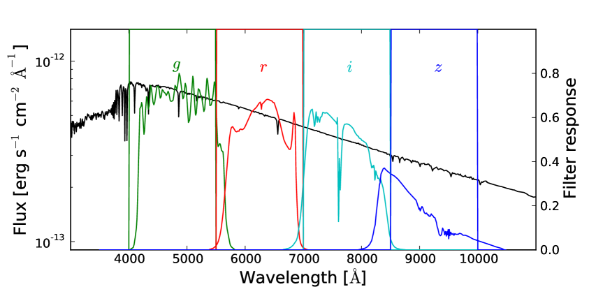
We start by determining how much the SALT2 parameters will be affected by a given modification in the reference spectrum BD+17${}^{\circ}\!$4708. This is done by refitting the SN Ia light curve data using a spectrum of BD+17${}^{\circ}\!$4708 which was perturbed using a step function, i.e. by increasing the flux by a factor $(1+\delta_{j})$ in four different wavelength ranges (one at a time) which roughly correspond to the wavelength coverage of the MegaCam $ugriz$ filter set shown figure 1. As an alternative to using step functions for the perturbation of the SED of BD+17${}^{\circ}\!$4708, we also tested perturbation bands with smooth edges. We replaced the sharp edge of the step functions with parabolic flanks of 250 Å width. The results for these perturbation bands differ only slightly from those for step functions. However, the functions avoid the complications due to overlapping bands. We chose the step functions for our default tests.

From this we determine the derivatives of the SALT2 parameters with respect to the perturbations $\delta_{i}$ with second-order numerical accuracy. We choose the MegaCam filters because a large fraction of the SNe we used either uses them (SNLS3 [15]) or uses similar filters (e.g. SDSS [30]). We make this specific choice of the perturbation bands so the results can be interpreted in a straight forward manner. Any other choice would be as valid. Note again that we perturb the SED of BD+17${}^{\circ}\!$4708 and not the zero points of the filters. Therefore the SNe with photometric data in other filter systems, e.g. BVRI, are affected by the perturbation as well. In section 3 the derivatives are used as part of data quality cuts, results and behaviour of the derivatives for the data set are discussed in section 4.1.

Figure 1: Perturbation bands compared to the MegaCam response functions [15] and the spectrum of BD+17${}^{\circ}\!$4708 (CALSPEC, as used by SALT2 [22])

We include the perturbations in the distance modulus (2) by linearizing their effect on light-curve parameters:

$$\mu^{\prime}=\mu+\sum\limits_{j}\frac{\partial m_{B}}{\partial\delta_{j}}\cdot\delta_{j}+\alpha\sum\limits_{j}\frac{\partial x_{1}}{\partial\delta_{j}}\cdot\delta_{j}-\beta\sum\limits_{j}\frac{\partial c}{\partial\delta_{j}}\cdot\delta_{j}$$ (2.3)

The cosmological fit (2.2) is modified to include the perturbations as parameters by replacing $\boldsymbol{V}$ and $\boldsymbol{X}$ with:

$$\boldsymbol{V^{\prime}}=\begin{pmatrix}\boldsymbol{V}\\ \boldsymbol{V}\delta_{g}\\ \boldsymbol{V}\delta_{r}\\ \vdots\end{pmatrix}=\begin{pmatrix}-\beta\\ 1\\ \alpha\\ -\beta\delta_{g}\\ \delta_{g}\\ \alpha\delta_{g}\\ \vdots\end{pmatrix},\quad\boldsymbol{X^{\prime}}=\begin{pmatrix}\boldsymbol{X}\\ \partial_{g}\boldsymbol{X}\\ \partial_{r}\boldsymbol{X}\\ \vdots\end{pmatrix}=\begin{pmatrix}c\\ m_{B}\\ x_{1}\\ \frac{\partial c}{\partial\delta_{g}}\\ \frac{\partial m_{B}}{\partial\delta_{g}}\\ \frac{\partial x_{1}}{\partial\delta_{g}}\\ \vdots\end{pmatrix},$$ (2.4)

thus extending the set of nuisance parameters by the perturbations $\delta_{j}$.

A similar technique was used in [14] to assess the systematic uncertainties due to calibration errors. However, there the aim was not to constrain the uncertainties of the reference spectrum, but to propagate the systematic uncertainties properly. In that analysis the light-curve template of SALT2 was retrained for each perturbed reference spectrum. We omit this step as training a light-curve template is beyond the scope of this work. We note, however, that this simplification is justified because the retraining of the template increases the effects of the perturbations only by $\sim\!5\%$ (A. Conley, private communication, 2011): the degeneracy between our nuisance parameters and the light-curve model, most notable the colour relations of the SN Ia light-curve, is expected to be small since the nuisance parameters are measured in the observer frame while the SN colour relations are given in the rest-frame. Hence, by using the full available redshift range, this affect should largely average out. Finally, we can test the validity of this approximation by comparing our cosmological results for a self-calibrating fit to some of the results found in [14] which include the systematic errors from uncertainties in the reference star colours (see section 4.2).

3 Data set and selection

For the method to work, the SN data set should be distributed over a large redshift range. Therefore we chose the Union2 data set [12] for our analysis which we expanded by 166 new SNe from the SNLS 3 year release [13] using only those not classified as SNe Ia$\star$. (SNe Ia$\star$ correspond to Confidence Index 3 of [31], i.e. the spectrum matches a SN Ia better than any other SN type, but another SN type — usually SNe Ic — is not ruled out from the spectrum alone.)

After fitting all light curves using SALT2 we followed the framework used in [12] to ensure sufficient quality of the data. All SNe are required to meet the Union2 criteria: (1) There is data from at least two bands with rest-frame wavelength between 3000 Å and 7000 Å, i.e. the default SALT2 wavelength range. This is very important for our analysis because the number of available bands affects the precision with which the SALT2 colour is determined. (2) There are at least five photometric measurements (3) There is at least one measurement between -15 and 6 (rest frame) days relative to the $B$-band maximum; (4) The fit values for $x_{1}$, including the fit uncertainties, lie between $-5<x_{1}<5$; (5) The CMB-centric redshift is greater than $z>0.015$.

To this list of requirements we add our own. As described in section 2, we include the effects of the perturbation of BD+17${}^{\circ}\!$4708 to our fit by linearizing them according to equation (2.3). For the linearization to be justified, we require that the quadratic terms in the Taylor expansion and hence the second derivatives are small. The quadratic term for e.g. the colour perturbed in $r$ is $\frac{1}{2}\frac{\partial^{2}c}{\partial\delta_{r}^{2}}\cdot\delta_{r}^{2}.$

While the light curve fits result in a first derivative that is $\lesssim\!1$ for all SNe as well as a similarly small second derivative for most SNe, there are some cases for which the second derivative is much larger, in a few cases even $>\!1000$. Such large second derivatives appear only for SNe with few photometric measurements. For a typical uncertainty of $\delta\!=\!1\%$, both the linear and quadratic terms are the same order of magnitude for a second derivative of about 200. We hence require of each SNe that the absolute values of its second derivatives $|\partial^{2}m_{B}/\partial\delta_{j}^{2}|$, $|\partial^{2}c/\partial\delta_{j}^{2}|$ and $|\partial^{2}x_{1}/\partial\delta_{j}^{2}|$ are smaller than 200. So this cut is chosen so that the quadratic term is at most the same size as the linear term.

After quality cuts there are 538 SNe from Union2 and 161 SNe from SNLS3 in our data set, 11 SNe are solely excluded because of non-linearity (9 for Union2 and 2 for SNLS3). Note that of the 569 SNe in Union2 before the $3\sigma$-clipping, 22 were excluded beforehand. These SNe all have photometric measurements in filter systems for which the zero points for BD+17${}^{\circ}\!$4708 could not be determined reliably.

To clean the data from outliers, the robust $3\sigma$-clipping as in [9] was adopted: the data set was first fit using median statistics [32] with $\mathcal{M}$ as the only free parameter (using $\alpha=0.12$ and $\beta=2.51$ as well as a flat cosmology with $\Omega_{\textrm{M}}=0.281$ (values taken from [12]) with $\sigma_{\textrm{int}}=0.1$). SNe outside a $3\sigma$ range were then excluded. Note that median statistics were only used to exclude outliers, for further fits we minimized $\chi^{2}$ according to eq. (2.2). This procedure leaves 501 SNe in Union2 and 158 in SNLS3 and thus a total of 659 SNe for our analysis. Note that considerably more SNe were rejected than the 12 SNe in [12]. This is due to the simplified approach undertaken here: The clipping was not done separately for each sample (and not using different $\sigma_{\textrm{int}}$), but for the whole data set at once. We note that the aim of this work is the first application of a method to incorporate systematic errors and not a new determination of cosmological parameters.

4 Results

4.1 Light-curve fits for the perturbed reference spectrum

Figure 2: Derivatives of the peak magnitude $m_{\textrm{B}}$ w.r.t. the perturbations. The colours and marker shapes indicate the number of bands from which data was available and in the default wavelength range of SALT2 (3000 Å to 7000 Å): 2 (red dots), 3 (orange circles), 4 or more (green crosses).

Figure 3: Derivatives of the colour $c$ w.r.t. the perturbations. Colours and marker as in figure 2.

Figure 4: Derivatives of the stretch parameter $x_{1}$ w.r.t. the perturbations. Colours and markers as in figure 2.

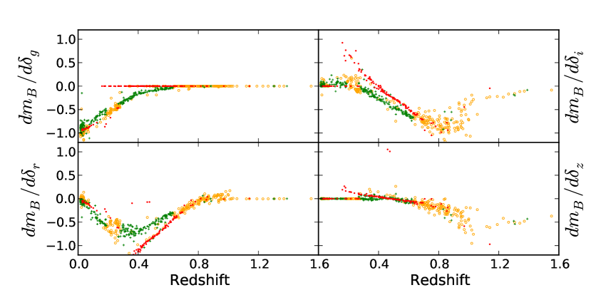
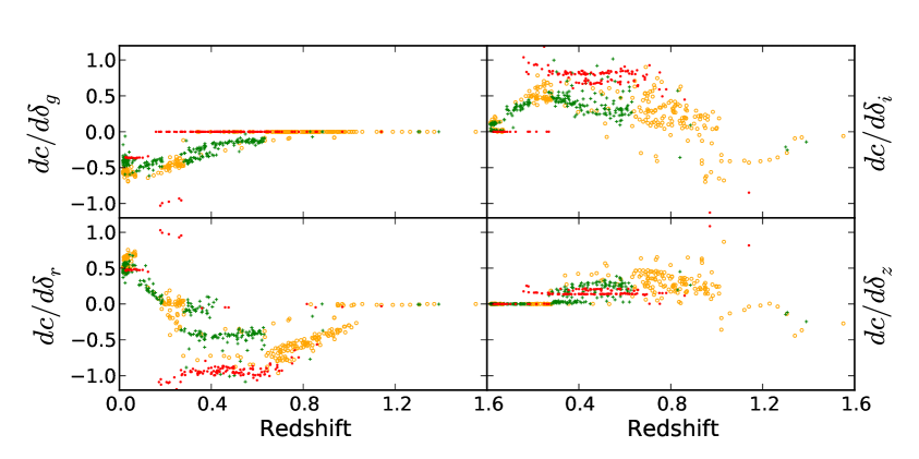
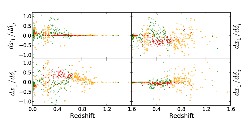
The behaviour of the light-curve fit results under perturbation of BD+17${}^{\circ}\!$4708 differs greatly from SN to SN. This is expected, as the effects of the perturbation depend on the redshift of the SN as well as the number of bands for which data is available. Figures 2–4 show the derivatives of the light-curve parameters with respect to the perturbations in a given band. We also tested perturbations of 2% and 3%, but the change of the derivatives is insignificant. Hence we used derivatives calculated form 1% perturbations throughout our analysis. A general behaviour can be observed that matches the expectations well. Firstly, there is a redshift dependence of the effects: Perturbations in $g$ have the greatest effect on low-redshift SNe, whereas perturbing $r$ and $i$ affects intermediate redshifts and $z$ takes effect for high redshifts. Secondly, the number of available bands influences the strength of the effect. Generally the perturbation will cause a smaller change in the fit parameters if the number of bands is larger.

Increasing the flux of BD+17${}^{\circ}\!$4708 causes the peak magnitude $m_{\textrm{B}}$ to drop for most of the SNe because the light-curve points are interpreted as being brighter. This means that the derivative $\partial m_{B}/\partial\delta_{j}$ (see figure 2) is negative and its value is expected to be between -1 and 0. We also see the aforementioned dependence on the number of bands: when perturbing $r$, the drop in $m_{B}$ is larger if only two bands are available because a greater fraction of light-curve points are affected by the perturbation than if more bands were given. When perturbing in $g$ on the other hand, most SNe with two bands are unaffected by the perturbation since these SNe only have photometric measurements in $R$ and $I$ which do not overlap with $g$.

The SALT2 colour parameter $c$ shows a similar behaviour. Hence values for $\partial c/\partial\delta_{j}$ (see figure 3) are expected to be between -1 and 1 with a clear redshift dependence. We observe that the effects are very similar for adjacent bands but have opposite signs and have the same dependence on the number of bands as $\partial m_{B}/\partial\delta_{j}$. These effects are best explained with a simple example: at redshift $z=0.45$ $r$ roughly correspond to the $B$ band, hence perturbing the spectrum of BD+17${}^{\circ}\!$4708 by 1% in $r$ decreases $B$ by 0.01 which in turn decreases $B-V$ by 0.01. Perturbing $i$ on other hand would decrease $V$ and thus increase $B-V$. So far in this analysis we assumed that only one colour (i.e. two bands) is available but if $U-B$ is also measured, it will increase when $r$ is perturbed and lessen the total change in $c$. Additionally we notice a sudden drop in $\partial c/\partial\delta_{r}$ around $z\sim\!0.63$ which coincides with a decrease of the number of bands from four to three. These SNe are all from SNLS. At $z\gtrsim 0.63$ the effective wavelength of the MegaCam-$g$ band corresponds to a rest-frame wavelength below 3000 Å and hence is ignored by SALT2.

An effect on the shape parameter $x_{1}$ can also be observed. However, this effect is more complicated than the effect on the other parameters, as the effect of the perturbations on the shape of the light-curve depends strongly on the number of light-curve points that were measured and on how the measurements are distributed relative to the peak.

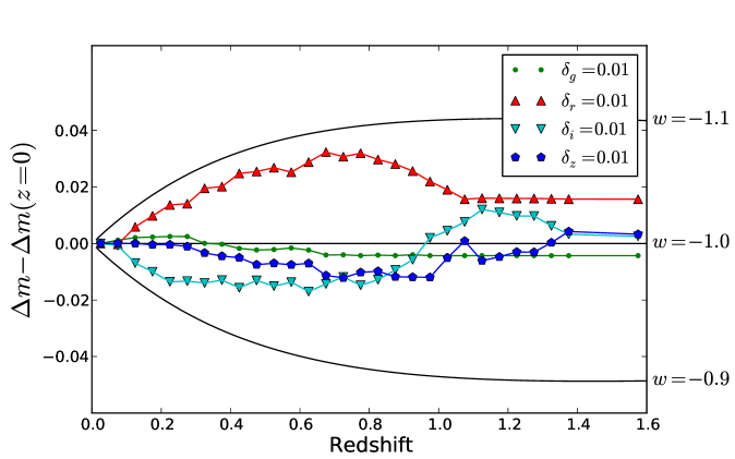
We can now combine the terms according to equation (2.3), using $\alpha=0.127$ and $\beta=2.802$. These values were determined in a cosmological fit of the data as described in section 4.2. Figure 5 shows the total effect of perturbations of 1% on the corrected magnitude. We averaged the values in redshift bins of the size $\Delta z=0.05$. Note that the values were shifted by $\Delta m_{g}=0.004,\Delta m_{r}=-0.016$ and $\Delta m_{i}=-0.002$ such that they meet at $z=0$. This is justified because cosmological parameters are anchored by nearby SNe. Shifting the magnitudes of nearby SNe changes results for the absolute magnitude of SNe Ia and hence changes $\mathcal{M}$ in a cosmology fit by a similar amount. For perturbations in the $z$-band no such shift was necessary as low-redshift SNe are not affected by the perturbation.

The largest effect is seen in $r$ and $i$ which is expected because all SNe are affected by perturbing those bands. For $g$ and $z$ some SNe have no measurements that are affected by the perturbation. Further the plot shows $\Delta m$ for different values of $w$ around a fiducial flat wCDM model with $\Omega_{\textrm{M}}=0.281$ and $w=-1$. This shows that changing $w$ by 0.1 changes $\Delta m$ by 0.04 for redshifts above $z\gtrsim 0.6$. The effect of perturbing $r$ alone is $\Delta m\sim\!0.03$. Hence we can predict a systematic uncertainty of $\sim\!0.075$ in $w$ for a 1% uncertainty in $r$ alone.

Figure 5: Change of the corrected magnitude for a 1% perturbation in a given filter. Note that the values were shifted such that the lowest redshift bin is at zero. The values of $\Delta m(z=0)$ are 0.004, -0.016, -0.002 and 0 for $g$, $r$, $i$, and $z$, respectively.

4.2 Cosmological fits

		$\chi^{2}$	$w$	$\mathcal{M}$	$\delta_{g}$	$\delta_{r}$	$\delta_{i}$	$\delta_{z}$
		662.2	-0.968(45)	-19.075(12)	–	–	–	–
one band	$g$	662.12	-0.962(50)	-19.071(18)	0.006(23)	–	–	–
	$r$	661.68	-1.027(96)	-19.090(24)	–	0.008(11)	–	–
	$i$	662.12	-0.975(54)	-19.074(13)	–	–	-0.002(10)	–
	$z$	658.69	-1.053(67)	-19.082(13)	–	–	–	-0.036(19)
two bands	$gr$	660.81	-1.069(108)	-19.089(24)	0.027(29)	0.016(15)	–	–
	$gi$	662.05	-0.969(58)	-19.071(19)	0.006(23)	–	-0.002(10)	–
	$gz$	657.61	-1.048(67)	-19.068(19)	0.025(24)	–	–	-0.043(21)
	$ri$	661.58	-1.039(103)	-19.097(33)	–	0.011(15)	0.004(13)	–
	$rz$	658.31	-1.105(110)	-19.095(25)	–	0.007(11)	–	-0.035(19)
	$iz$	656.6	-1.154(100)	-19.082(13)	–	–	-0.016(12)	-0.053(23)
three bands	$gri$	655.71	-1.539(236)	-19.205(47)	0.156(58)	0.107(35)	0.057(21)	–
	$grz$	654.11	-1.306(158)	-19.104(26)	0.072(35)	0.031(17)	–	-0.057(22)
	$giz$	654.76	-1.171(102)	-19.064(19)	0.033(25)	–	-0.019(12)	-0.067(25)
	$riz$	655.61	-1.097(109)	-19.044(40)	–	-0.019(20)	-0.032(20)	-0.071(30)

Table 1: Results of cosmology fits. The first line shows the standard fit, the blocks thereafter show self-calibrating fits for different numbers of perturbation bands. The results for the correction coefficients are $\alpha=0.127(6)$ and $\beta=2.802(58)$. Their values do not change significantly for self-calibrating fits.

The uncertainties of reference star colours have a large impact on the measurements of $w$. SNe alone cannot constrain $w$ and $\Omega_{\textrm{M}}$ very well at the same time. Therefore we only fit $w$ while assuming a flat universe with $\Omega_{\textrm{M}}=0.281$. This emulates the inclusion of BAO and CMB priors which constrain strongly $\Omega_{\textrm{M}}$. The choice of $\Omega_{\textrm{M}}$ is taken from [12]. A proper full analysis was beyond the scope of this paper. However, choosing a different $\Omega_{\textrm{M}}$ between 0.26 and 0.3 only changes the mean value of $w$ and does not affect its uncertainty. Recall that we are interested in the statistical behaviour of the uncertainties and not the mean values.

First we fit the cosmology without perturbations, i.e. minimizing $\chi^{2}$ as per equation (2.2). $\sigma_{\textrm{int}}$ was tuned to 0.115 which yielded $\chi_{\textrm{red}}^{2}=1.011$. For further fits $\sigma_{\textrm{int}}$ was kept at this value to ensure comparability. The top row of table 1 shows the resulting parameters for this fit. The table only shows the parameters $w$ and $\mathcal{M}$, the nuisance parameters $\alpha$ and $\beta$ were also determined in every fit but they do not change significantly in a self-calibrating fit. For the unperturbed fit we found $\alpha=0.127\pm 0.006$ and $\beta=2.802\pm 0.058$. The resulting value of $w$ is consistent with a cosmological constant. The error of $w$, $\sigma_{w}=0.045$, only contains the statistical uncertainty, not the systematic one.

Next, we included a single perturbation parameter in the fit while leaving the other bands as they are (see the first block in table 1). The resulting deviations are of the order of a few percent and consistent with zero. The interesting results are the uncertainties of $w$: While perturbing the $g$- and $i$-bands increases $\sigma_{w}$ only slightly, perturbing $r$ more than doubles the uncertainty. Also there is a larger change in $\sigma_{\mathcal{M}}$ for the $r$-band as well. This matches our predictions from figure 5. The overall change of $\Delta m$ is largest for the $r$-band and more importantly it is large for low redshift which changes $\mathcal{M}$. The self-calibrating fit already constrains the perturbation of the reference spectrum to about 1% in $r$ and $i$ and to about 2% in $g$ and $z$. It is noteworthy that the method already constrains the flux to a level that is compatible with the currently quoted uncertainties. The increase in measurement uncertainty due to self-calibration is given by

$$\Delta w=\sqrt{\sigma_{w}^{2}\textrm{(self-calibrating)}-\sigma_{w}^{2}\textrm{(unperturbed)}}.$$ (4.1)

This gives a $\Delta w=0.02$ for perturbations in $g$ and $\Delta w=0.085$ for $r$. The latter matches our predictions from figure 5 well. The confidence regions for the perturbed fits (see figures 6 and 7) show the same effect. While $\delta_{g}$ is less constrained than $\delta_{r}$, it has a smaller effect on the uncertainties in $w$ and $\mathcal{M}$.

Figure 6: 95% confidence regions for self-calibration in $g$ and $r$ compared to the unperturbed fit

Figure 7: 95% confidence regions for self-calibration in $i$ and $z$ compared to the unperturbed fit

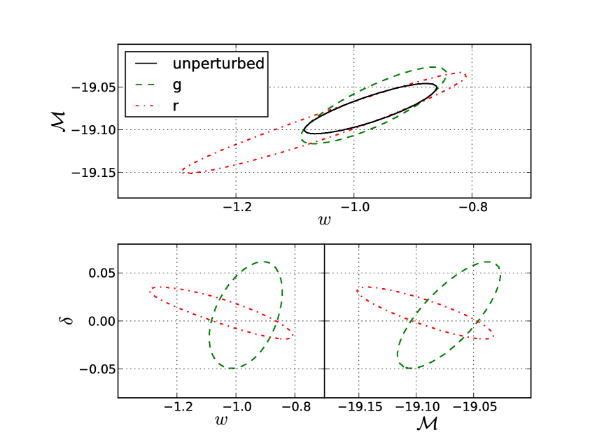
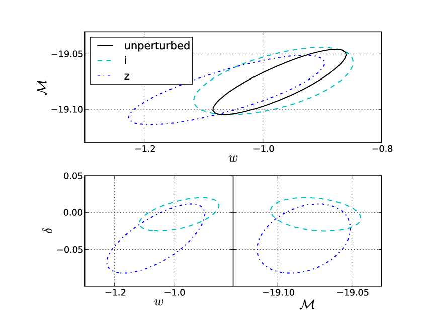
To verify that the omission of retraining the light-curve template is justified, we can compare the $\Delta w$ to the results found by SNLS [14] which include the systematic errors from uncertainties in the reference star colour. In [14] the uncertainties of the reference colours were marginalized over to include systematic uncertainties. Hence, this comparison is only valid for colours which have a systematic uncertainty that is at least the same order of magnitude as the constraints we determine using a self-calibrating fit. The only colour that meets this requirement is $z_{M}-V$ for which an uncertainty of 0.0178 was used [15]. In a cosmology fit with fixed $\Omega_{\textrm{M}}$ similar to ours this leads to an increase of the uncertainty in $w$ from 0.058 to 0.071 which corresponds to adding 0.041 quadratically. Therefore we find that our result for $z$ – a quadratic increase by 0.049 – is in good agreement with the systematic uncertainty found in [14]. However, given that $z$ contributes only at high redshifts and has typically a lower signal-to-noise ratio, this does not conclusively show that the effect of retraining is insignificant.

Next, two bands are included as perturbation parameters in the fit, see the second block of table 1. This adds another degeneracy because one perturbation might cancel out the others effect on the colour. For some combinations of bands ($gr$, $gz$, $iz$) the mean values of both parameters increases. For the other combinations ($ri$, $rz$, $gi$) they do not change, nor do the uncertainties change much. There are two reasons for this stability. Firstly, non-adjacent bands are more stable because increasing two adjacent bands result in virtually no change of the colour. Secondly, the inner bands $r$ and $i$ are better constrained and hence help to constrain the other band.

Furthermore it is possible to include three perturbation parameters (see the third block of table 1), while including all four bands would create an almost perfect degeneracy to $\mathcal{M}$ because increasing all $\delta$s by the same amount can the absorbed by increasing $\mathcal{M}$ as well. Hence, in our analysis one band needs to be left unperturbed. This band should be in the middle of the wavelength range, so only two bands are adjacent. Thus we left the $r$-band fixed while $g$, $i$ and $z$ were perturbed. For this fit we get $w=-1.166\pm 0.101$.

4.3 Extrapolation to larger data sets

Figure 8: Extrapolated uncertainty in $w$ for the self-calibrating fit and the unperturbed fit with 4% systematics. The number of SNe at which the self-calibrating fit is expected to be more precise is $N_{\textrm{eq}}\sim\!3500$. Note that the mean points are highly correlated as the are calculated from the same data set split randomly in smaller samples.

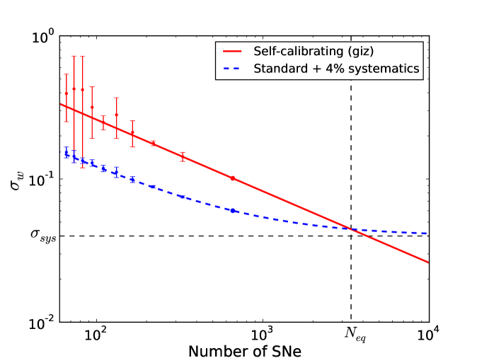
As a next step we tested if the uncertainties behave in a statistically sound fashion by splitting the data set randomly into several smaller samples, i.e. two samples of 330 SNe, three of 220 SNe and so on. For the unperturbed fit we clearly observe that the statistical uncertainty $\sigma_{w}$ decreases with $1/\sqrt{N}$ but for the self-calibrating fits the uncertainties can vary greatly from one random realization to the other. We calculated the mean uncertainties for each sample size taking their standard deviation as an error. Figure 8 shows this for the unperturbed fit and a self-calibrating fit in $g$, $i$ and $z$. Note that we add a constant uncertainty $\sigma_{\textrm{sys}}=0.04$ to the result of the unperturbed fit (see below). The behaviour of the uncertainties, when compared with the $1/\sqrt{N}$ predicted scaling, confirms that the data set behaves statistically sound in the self-calibrating fit.

We can extrapolate the uncertainties for larger data sets. If the calibration does not improve, the systematic uncertainty on $w$ will stay at the current value of about $\sigma_{\textrm{sys}}=0.04$ which is the systematic error currently found in cosmological analyses [12, 14]. Therefore $\sigma_{w}$ will approach this value asymptotically and not improve beyond that. The uncertainty from a self-calibrating fit, however, contains the calibration error and will keep decreasing with larger numbers of observed SNe. Figure 8 shows uncertainties from unperturbed and self-calibrating fits and the extrapolation of $\sigma_{w}$ for larger surveys. Based on this, we find that for number of observed SNe $N_{\textrm{SNe}}\sim\!3500$, a self-calibrating fit will reach the same precision as the unperturbed fit with systematics. Beyond that, our method will be outperforming the conventional method of treating the uncertainty.

5 Discussion and conclusion

In this paper we have applied the method of a self-calibrating Hubble diagram to existing data for the first time to constrain uncertainties in the flux measurements of the fundamental flux standard. To construct a self-calibrating Hubble diagram, the SN light-curve data is refit using SALT2 with a perturbed reference spectrum in which the flux was increased or decreased slightly in a certain redshift range. The change of the light-curve fit results due to this perturbation can then be linearized and included in the Hubble fit, using the strength of the perturbation as a nuisance parameter.

Our analysis has shown that a self-calibrating approach to incorporating calibration uncertainties works well with the current SN Ia data sets. The self-calibrating Hubble diagram can be constructed for any compilation of data from various surveys as the photometric measurements are compared relative to a single reference star. However, we identified non-linear effects of the perturbation of the reference spectrum as an issue for using this method with the current data and included a quality cut for this in the data selection framework accordingly. Also we have omitted the retraining of the SN Ia light-curve template. Based on a related study this is only a 5% effect and hence will not alter the conclusions significantly. However, for a future study of the self calibration method, it would be appropriate to further investigate the role of the light curve training.

Self-calibrating Hubble fits for the current data can already constrain the uncertainties for the spectrum of BD+17${}^{\circ}\!$4708 to almost the same level as found in the literature, where the spectrum was calibrated using three white dwarfs. Only for shorter wavelengths, i.e. the $g$-band, these constraints are not that tight because the redshift range usable for self-calibration is limited. When using more than one perturbation parameter in the fit, degeneracies between the parameters can appear. Even though they increase the penalty of self-calibration at the current number of SNe, the uncertainties behave in a statistically sound fashion. Therefore the uncertainties can still be expected to decrease when larger data sets become available. Extrapolations from the results for current data show that the self-calibrating Hubble diagram will outperform the standard method when the number of observed SNe has grown by about a factor of five, i.e. $\sim\!3500$ SNe are available. This number of SN observation will be achieved by upcoming surveys such as DES and LSST. In this prediction, several simplifications were made which might influence the number of SNe that will actually be required. Simply scaling the uncertainties, implicitly assumes that the accuracy of the CMB and BAO priors will also improve similarly within the next decade. This is justified as surveys to improve CMB and BAO results are already underway, e.g. Planck or BigBOSS. Also the quality of the data taken by future surveys will be better than the average quality of the data set used here. Using more SN light-curve data with smaller uncertainties (especially at low or high redshifts) will constrain the uncertainties of the primary reference star better than extrapolated by simply scaling the uncertainties. Furthermore this work only used SNe with spectroscopic redshifts but future surveys will also rely on photometric redshift determinations. In that case, calibration uncertainties will also affect the resulting redshifts. This effect will have to be analysed with techniques similar to those presented here.

When constraining the calibration uncertainties using the self-calibration method, one makes use of the assumption that SNe Ia are truly standardizable and therefore do not evolve with redshift. More precisely, the method requires that the rest-frame colour relations remain the same for all redshifts. However, a change in the metallicity, for instance, can have a greater effect on the rest-frame $U$-band than on redder bands (see e.g. [29]). This change in the colour relations will be partially absorbed during the self-calibration procedure, which potentially can lead to a wrong interpretation of the resulting cosmological parameters and affect the nuisance parameters in the self-calibrating fit. Consequently any significant departure of a nuisance parameter from zero would need to be investigated carefully for evolution effects, e.g. by separating the SNe by host type and/or SN characteristics, as well as possible survey specific effects that can be investigated by subdividing the data according the surveys.

In our analysis we have only constrained the uncertainties of the SED of BD+17${}^{\circ}\!4708$. With the framework presented here, it is also possible to constrain the zero points of individual surveys, however, at the potential expense of more nuissance parameters. Once sufficiently large SN data sets from single surveys become available (e.g. $\sim 10^{5}$ SNe from LSST), that do not require the combination with other samples, perturbing the zero point will have the same effect on the cosmological fit results as perturbing the reference spectrum. Hence, it will not further worsen the constraints on $w$, while absorbing another significant source of systematic error.

References

- [1] S. Perlmutter et. al., Discovery of a supernova explosion at half the age of the universe, Nature 391 (Jan., 1998) 51–+, [astro-ph/9712212].
- [2] P. M. Garnavich et. al., Supernova Limits on the Cosmic Equation of State, ApJ 509 (Dec., 1998) 74–79, [astro-ph/9806396].
- [3] B. P. Schmidt et. al., The High-Z Supernova Search: Measuring Cosmic Deceleration and Global Curvature of the Universe Using Type IA Supernovae, ApJ 507 (Nov., 1998) 46–63, [astro-ph/9805200].
- [4] A. G. Riess et. al., Observational Evidence from Supernovae for an Accelerating Universe and a Cosmological Constant, AJ 116 (Sept., 1998) 1009–1038, [astro-ph/9805201].
- [5] S. Perlmutter et. al., Measurements of Omega and Lambda from 42 High-Redshift Supernovae, ApJ 517 (June, 1999) 565–586, [astro-ph/9812133].
- [6] R. A. Knop et. al., New Constraints on , , and w from an Independent Set of 11 High-Redshift Supernovae Observed with the Hubble Space Telescope, ApJ 598 (Nov., 2003) 102–137, [astro-ph/0309368].
- [7] P. Astier et. al., The Supernova Legacy Survey: measurement of , and w from the first year data set, A&A 447 (Feb., 2006) 31–48, [astro-ph/0510447].
- [8] W. M. Wood-Vasey et. al., Observational Constraints on the Nature of Dark Energy: First Cosmological Results from the ESSENCE Supernova Survey, ApJ 666 (Sept., 2007) 694–715, [astro-ph/0701041].
- [9] M. Kowalski et. al., Improved Cosmological Constraints from New, Old, and Combined Supernova Data Sets, ApJ 686 (Oct., 2008) 749–778, [arXiv:0804.4142].
- [10] M. Hicken et. al., Improved Dark Energy Constraints from New CfA Supernova Type Ia Light Curves, ApJ 700 (Aug., 2009) 1097–1140, [arXiv:0901.4804].
- [11] R. Kessler et. al., First-Year Sloan Digital Sky Survey-II Supernova Results: Hubble Diagram and Cosmological Parameters, ApJS 185 (Nov., 2009) 32–84, [arXiv:0908.4274].
- [12] R. Amanullah et. al., Spectra and Hubble Space Telescope Light Curves of Six Type Ia Supernovae at and the Union2 Compilation, ApJ 716 (June, 2010) 712–738, [arXiv:1004.1711].
- [13] J. Guy et. al., The Supernova Legacy Survey 3-year sample: Type Ia supernovae photometric distances and cosmological constraints, A&A 523 (Nov., 2010) A7+, [arXiv:1010.4743].
- [14] A. Conley et. al., Supernova Constraints and Systematic Uncertainties from the First Three Years of the Supernova Legacy Survey, ApJS 192 (Jan., 2011) 1–+, [arXiv:1104.1443].
- [15] N. Regnault et. al., Photometric Calibration of the Supernova Legacy Survey Fields, A&A 506 (Aug., 2009) 999.
- [16] R. C. Bohlin and R. L. Gilliland, Hubble Space Telescope Absolute Spectrophotometry of Vega from the Far-Ultraviolet to the Infrared, AJ 127 (June, 2004) 3508–3515.
- [17] A. U. Landolt, UBVRI photometric standard stars in the magnitude range 11.5-16.0 around the celestial equator, AJ 104 (July, 1992) 340–371.
- [18] Ž. Ivezić et. al., Sloan Digital Sky Survey Standard Star Catalog for Stripe 82: The Dawn of Industrial 1% Optical Photometry, AJ 134 (Sept., 2007) 973–998, [astro-ph/].
- [19] N. Padmanabhan et. al., An Improved Photometric Calibration of the Sloan Digital Sky Survey Imaging Data, ApJ 674 (Feb., 2008) 1217–1233, [astro-ph/].
- [20] A. G. Kim and R. Miquel, Optimal extraction of cosmological information from supernova data in the presence of calibration uncertainties, Astroparticle Physics 24 (Jan., 2006) 451–458, [astro-ph/].
- [21] L. Faccioli et. al., Reducing zero-point systematics in dark energy supernova experiments, Astroparticle Physics 34 (July, 2011) 847–857, [arXiv:1004.3511].
- [22] J. Guy et. al., SALT2: using distant supernovae to improve the use of type Ia supernovae as distance indicators, A&A 466 (Apr., 2007) 11–21, [astro-ph/0701828].
- [23] M. M. Phillips, The absolute magnitudes of Type IA supernovae, ApJ 413 (Aug., 1993) L105–L108.
- [24] A. G. Riess, W. H. Press, and R. P. Kirshner, Using Type IA supernova light curve shapes to measure the Hubble constant, ApJ 438 (Jan., 1995) L17–L20, [astro-ph/].
- [25] S. Perlmutter et. al., Measurements of the Cosmological Parameters Omega and Lambda from the First Seven Supernovae at 0.35, ApJ 483 (July, 1997) 565–+, [astro-ph/].
- [26] R. Tripp, A two-parameter luminosity correction for Type IA supernovae, A&A 331 (Mar., 1998) 815–820.
- [27] A. G. Riess, W. H. Press, and R. P. Kirshner, A Precise Distance Indicator: Type IA Supernova Multicolor Light-Curve Shapes, ApJ 473 (Dec., 1996) 88–+, [astro-ph/].
- [28] J. Guy et. al., SALT: a spectral adaptive light curve template for type Ia supernovae, A&A 443 (Dec., 2005) 781–791, [astro-ph/].
- [29] N. Chotard et. al., The reddening law of type Ia supernovae: separating intrinsic variability from dust using equivalent widths, A&A 529 (May, 2011) L4, [arXiv:1103.5300].
- [30] M. Fukugita et. al., The Sloan Digital Sky Survey Photometric System, AJ 111 (Apr., 1996) 1748–+.
- [31] D. A. Howell et. al., Gemini Spectroscopy of Supernovae from the Supernova Legacy Survey: Improving High-Redshift Supernova Selection and Classification, ApJ 634 (Dec., 2005) 1190–1201, [astro-ph/0509195].
- [32] J. R. Gott, III et. al., Median Statistics, H0, and the Accelerating Universe, ApJ 549 (Mar., 2001) 1–17, [astro-ph/].