The Effects of Anisotropic Viscosity on Turbulence and Heat Transport in the Intracluster Medium
Abstract
In the intracluster medium (ICM) of galaxy clusters, heat and momentum are transported almost entirely along (but not across) magnetic field lines. We perform the first fully self-consistent Braginskii-MHD simulations of galaxy clusters including both of these effects. Specifically, we perform local and global simulations of the magnetothermal instability (MTI) and the heat-flux-driven buoyancy instability (HBI) and assess the effects of viscosity on their saturation and astrophysical implications. We find that viscosity has only a modest effect on the saturation of the MTI. As in previous calculations, we find that the MTI can generate nearly sonic turbulent velocities in the outer parts of galaxy clusters, although viscosity somewhat suppresses the magnetic field amplification. At smaller radii in cool-core clusters, viscosity can decrease the linear growth rates of the HBI. However, it has less of an effect on the HBI’s nonlinear saturation, in part because three-dimensional interchange motions (magnetic flux tubes slipping past each other) are not damped by anisotropic viscosity. In global simulations of cool core clusters, we show that the HBI robustly inhibits radial thermal conduction and thus precipitates a cooling catastrophe. The effects of viscosity are, however, more important for higher entropy clusters. We argue that viscosity can contribute to the global transition of cluster cores from cool-core to non cool-core states: additional sources of intracluster turbulence, such as can be produced by AGN feedback or galactic wakes, suppress the HBI, heating the cluster core by thermal conduction; this makes the ICM more viscous, which slows the growth of the HBI, allowing further conductive heating of the cluster core and a transition to a non cool-core state.
keywords:
convection—galaxies: clusters: intracluster medium—instabilities—turbulence—X-rays: galaxies: clusters1 Introduction
Clusters of galaxies are the largest gravitationally bound objects in the universe, and as such, they potentially provide sensitive tests of cosmological parameters. They are filled with a hot, dilute, magnetized plasma, the intracluster medium (ICM), that emits copious X-rays. Observations of the ICM provide an interesting and unique window on problems ranging from constraining dark energy to understanding the accretion and feedback processes for supermassive black holes.
The plasma in the ICM has temperatures ranging from 1–15 keV and number densities from to . This dilute plasma has a magnetic field that has been estimated to range from 0.1–10 G (Carilli & Taylor, 2002). With these parameters the mean free path of electrons along the magnetic field line is times larger than the gyroradius at all radii in the ICM. Ions have a similar separation of scales. The mean free path is, however, always shorter than the local scale height; therefore, a fluid description of the plasma (as opposed to a collisionless description) is appropriate and the ICM can be described by the Braginskii-MHD equations (Braginskii, 1965). These equations are the standard ideal MHD equations supplemented with anisotropic conduction due to the electron heat flux and anisotropic momentum transport due to the ion viscosity along the magnetic field. In the ICM, transport perpendicular to the local magnetic field is negligible.
As a result of the anisotropic heat transport in the ICM, the Schwarzschild criterion for convective instability—that the entropy increase in the direction of gravity—is replaced by a criterion on temperature. In recent years, two buoyant instabilities have been discovered that drive convection with the temperature gradient as a source of free energy. The first instability, the magnetothermal instability (MTI), was described in Balbus (2000) and has been simulated in two and three dimensions (Parrish & Stone, 2005, 2007; McCourt et al., 2011a). The MTI is unstable when the temperature gradient and gravity are in the same direction and grows fastest for a magnetic field perpendicular to gravity. The MTI operates in the outskirts of galaxy clusters and has been found to drive vigorous convection that can provide over 30% of the pressure support near the virial radius (Parrish et al., 2011). The second instability, the heat-flux-driven buoyancy instability (HBI) was described in Quataert (2008) and has been simulated in local simulations in 2D and 3D (Parrish & Quataert, 2008). The HBI is unstable when the temperature gradient and gravity point in opposite directions and has the fastest growth for a magnetic field parallel to gravity. The HBI operates in the centers of cool-core clusters and saturates by reorienting the magnetic field to be perpendicular to gravity, greatly reducing the effective radial conductivity and hastening a cooling catastrophe (Parrish et al., 2009; Bogdanović et al., 2009). The interaction of the HBI with turbulence can help explain the bimodality observed between cool core and non-cool core clusters (Parrish et al., 2010; Ruszkowski & Oh, 2010).
None of these previous numerical studies have self-consistently included viscosity because the ratio of viscous to thermal diffusion, the Prandtl number,111This quantity should not be confused with the often-discussed magnetic Prandtl number in which the thermal diffusivity is replaced by the electrical resistivity. The magnetic Prandtl number is very large in the ICM. for a hydrogenic plasma is
| (1) |
where and are the diffusion coefficients for momentum (by ions only) and thermal energy (by electrons only), respectively. Pr is relatively small, and thus the effects of viscosity were expected to be small in comparison with those of conduction.222The effective value of the Prandtl number that enters the perturbed total energy equation in the linear analysis corresponds to . This is because : only electrons participate in conduction, while both electrons and ions contribute to the total thermal energy. The net effect is that is smaller for the MHD fluid by a factor of 2. In our calculations we take and . However, the Reynolds number is fairly small in the ICM:
| (2) |
and thus it is not so clear that the effects of viscosity can be neglected. Kunz (2011) (hereafter K11) recently extended the linear dispersion relation for the MTI and HBI to include anisotropic viscosity and provides an intuitive, physical explication of its effects. The most important is that the growth rates of the HBI can be suppressed by viscosity in the limit of very rapid conduction (and thus very rapid viscous damping). Isotropic viscosity has been utilized in a small number of previous numerical studies; e.g., Reynolds et al. (2005) studied the effect of viscosity on the shapes of rising AGN-blown bubbles. More recently, Dong & Stone (2009) showed that it is critical to consider anisotropic viscosity, rather than isotropic viscosity, in such calculations because the former is much less effective at suppressing the Rayleigh-Taylor instability.
In this paper, we present fully self-consistent 2D and 3D Braginskii-MHD simulations of the ICM, focusing on the evolution of the MTI and HBI. We introduce our computational methods in §3. In §4 we present local 2D and 3D simulations of the HBI and MTI to provide physical insight into the role of viscosity. We then use global calculations to study the effect of viscosity on the MTI in the outskirts of galaxy clusters and the role of the viscous HBI in cluster cores in §5 & §6, respectively. In the appendix we describe our numerical method for anisotropic viscous transport and discuss the numerical verification of this algorithm.
2 Method and Models
We solve the usual equations of magnetohydrodynamics (MHD) with the addition of anisotropic thermal conduction and anisotropic viscous transport. The MHD equations in conservative form are
| (3) |
| (4) |
| (6) |
which are the equations of conservation of mass, momentum, and energy and the induction equation, respectively. The total energy is given by
| (7) |
where . Throughout this paper, we assume . The anisotropic electron heat flux is given by
| (8) |
where is the Spitzer conductivity (Spitzer, 1962) and is a unit vector in the direction of the magnetic field. The Spitzer conductivity can be written as , where is the actual diffusion coefficient (in units of ). The viscous stress tensor is given by
| (9) |
where is the microphysical momentum diffusion coefficient, often termed the kinematic viscosity. Both transport coefficients are functions of temperature proportional to , where we presume . The microphysics fixes the ratio of the transport coefficients to be as given by Equation (1).
The energy equation also includes a cooling term, . The cooling function we adopt is from Tozzi & Norman (2001) with the functional form
| (10) |
with units of erg cm-3 s-1. The temperature dependence is a fit to cooling dominated by Bremsstrahlung above 1 keV and metal lines below 1 keV with
| (11) |
where , , and , for a metallicity of , with units of . We use a mean molecular weight of which corresponds to a metallicity of approximately solar.
For our simulations we use the Athena MHD code (Gardiner & Stone, 2008; Stone et al., 2008) combined with the anisotropic conduction methods of Parrish & Stone (2005) and Sharma & Hammett (2007). The anisotropic viscosity is implemented in a very similar manner to conduction (see the appendix). The heating, cooling, and anisotropic conduction and viscosity are operator split and sub-cycled with respect to the MHD timestep. The cooling simulations are implemented with a temperature floor of keV, below which UV lines become important, and the cooling curve fit is no longer accurate. This temperature floor prevents the cooling catastrophe from going to completion.
This paper will cover a variety of initial conditions from local Cartesian boxes to global cluster models. Our initial conditions will thus be described briefly in subsequent sections with appropriate references for more details. In each case, we have carried out a least one resolution study to assure numerical convergence. Any deviations will be noted.
3 Physics of the MTI and HBI with Viscosity
We begin with a qualitative description of the physics of the HBI and MTI. Despite the mathematical similarities of the instabilities, it is useful to discuss each instability separately. The MTI is most unstable for horizontal () magnetic fields with the temperature gradient . An upwardly displaced fluid element is connected by magnetic field lines to a hotter region deeper in the atmosphere. Heat flowing along the field expands the fluid element relative to its surroundings, lowers its density and buoyantly destabilizes the perturbation. The upward motion causes the magnetic field to be more aligned with the background temperature gradient, leading to an instability.
The HBI, on the other hand, is most unstable for vertical () magnetic fields with the temperature gradient . Imagine a small displacement of fluid elements with a wavevector that has a component both parallel and perpendicular to gravity (and ). This configuration, illustrated in Figure 1 of Quataert (2008), has regions in which the magnetic field lines bunch together and spread apart, leading to a converging and diverging heat flux. Rapid heat conduction along the perturbed magnetic field lines causes an upwardly displaced fluid element to be heated (by tapping into the background heat flux), leading to a buoyant runaway.
K11 carried out a full linear perturbation analysis on equations 3–8 and presents a dispersion relation for the MTI and HBI including the effects of anisotropic viscosity. For clarity when comparing with our results, we reproduce the K11 dispersion relation here in a slightly different coordinate system. We define gravity to be in the -direction, the initial magnetic field is in the - plane and is the component of the wavevector perpendicular to gravity. The dispersion relation for the growth rate, , is given by
where , and is the Alfvén velocity. The Brunt-Väisälä oscillation frequency is given by
| (13) |
where , and corresponds to buoyant oscillations in an unmagnetized plasma (g-modes). The characteristic frequency at which conduction and viscosity act are given by
| (14) | |||||
| (15) |
where is the thermal diffusivity and is the ion collision frequency. The buoyancy frequency is given by
| (16) |
which is roughly the fastest growth rate of the MTI or HBI. Finally, the dimensionless geometric factor is given by
| (17) |
where is the dimensionless magnetic field strength.
We can greatly simplify this expression and improve our physical intuition by assuming that the magnetic field is weak (or, equivalently, that the perturbation wavelength in the cluster core , where is a typical timescale for the instabilities to grow). We also assume the perturbation lies in the plane containing and , i.e. . In this limit, the dispersion relation simplifies to
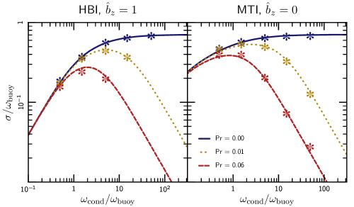
Without viscosity, there is a fast conduction limit in which the growth rate asymptotes to a constant ; with viscosity, however, no such limit exists. In Figure 1 we plot the theoretical curves for the growth rates of both the HBI and MTI as a function of the ratio for several Prandtl numbers. These curves assume a wave vector at 45 degrees from the magnetic field ; these represent typical, not maximum, growth rates. The ratio so that larger values of this ratio correspond physically to smaller scales at fixed conductivity.
Figure 1 shows that the inviscid solution reaches an asymptotic growth rate in the fast conduction limit; however, with viscosity the growth rate slowly decreases as one moves to the infinite conduction limit. For the HBI, the fastest growth occurs on scales satisfying , i.e., , and the maximum growth rate for is about 70% of the asymptotic inviscid value. This is independent of unless . For higher viscosities, the maximum growth rate scales as . The influence of viscosity on the MTI is much more modest. In particular, the fastest growing mode is achievable even for ; this is not seen in Figure 1 because of the particular perturbation chosen. One can, however, always find short wavelength MTI modes that grow at .
The microphysical plasma physics fixes the ratio of the diffusion coefficients, the Prandtl number (eqn. [1]), to be . This value corresponds to . Because there are MTI modes that grow rapidly even for , we would a priori not expect viscosity to have a significant effect on the evolution of the MTI. For the HBI, the viscous and inviscid growth rates are similar only when ; these larger scales in a physical system are only minimally affected by viscosity. We thus expect the HBI to be modified by viscosity only if on the largest scales of the system.
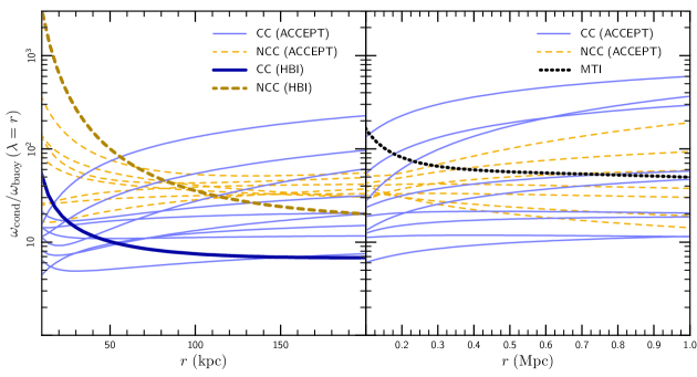
In Figure 2 we show the ratio of for observed clusters using as the conduction length scale and not including any geometric factors, i.e. . The left panel focuses on the core of the cluster where the HBI operates while the right panel is at larger radii where the MTI is present. The values of in Figure 2 are characteristic of the largest scales in the system. Smaller scales are more viscous/conducting, but are also where magnetic tension is most likely to suppress the MTI/HBI. Figure 2 also shows the ratio (defined in the same way) for our model clusters used in the global simulations in §5 & 6. The models are generally representative of real clusters.
The data in Figure 2 comes from the ACCEPT sample (Cavagnolo et al., 2009); the analysis of the data follows the methodology described in McCourt et al. (2011b) with the clusters listed in Table 2 of that work. These examples span relatively massive NCC clusters all the way down to groups. Cool-core (CC) clusters have –30 in the bulk of the core between a few–200 kpc. By comparing the real CC clusters to Figure 1 we see that viscosity only modestly reduces the growth rates of the HBI. Non-cool-core (NCC) clusters are more conducting/viscous as a result of the hotter and lower density cores. The effects of viscosity on the HBI are theoretically more likely to be significant in NCC clusters.
The star symbols in in Figure 1 show good agreement between the measured growth rates in our simulations and the analytic results; this represents a strong test of our algorithms for anisotropic conduction and viscosity. We discuss this in more detail in the appendix.
4 Local Simulations
4.1 Initial Conditions

It is illustrative to start with the simplest possible experiments, namely local two- and three-dimensional boxes with system sizes the scale-height . For this section we work in units with , , and with a hydrogenic plasma that has . Our initial conditions are fully detailed in McCourt et al. (2011a). For the HBI, we start with a simple hydrostatic equilibrium that is linearly unstable:
| (19) | |||||
| (20) |
where we set and choose a scale height of . Our boxes are of size in each dimension with a resolution of or . Results at this resolution are very well converged by all metrics. The vertical boundary conditions fix the temperature to its initial value, and the horizontal boundary conditions are periodic. The initial magnetic field is weak and vertical, .
For the local MTI simulations we utilize the set-up from §3.3 of McCourt et al. (2011a) given by
| (21) | |||||
| (22) |
with and . We select and solve numerically for to ensure hydrostatic equilibrium. These boxes are of size with an initially weak horizontal magnetic field, . Convergence is a bit more subtle in these simulations, but is reasonably well-converged (McCourt et al., 2011a).
For the HBI, the atmosphere satisfies the Schwarzschild criterion () and would be buoyantly stable in the absence of anisotropic conduction. In these calculations we fix the diffusivities so that the conduction frequency across the box is a chosen constant relative to the buoyancy frequency, and show results for different values of for both the inviscid case and the physical case with .
4.2 Nonlinear Saturation
4.2.1 HBI
We begin by examining the nonlinear saturation of the HBI with 2D single mode simulations. The magnetic field lines from these simulations are visualized in Figure 3. Each vertical column compares inviscid and viscous simulations at the time . This is well into the non-linear regime, in which the statistical properties of the plasma do not evolve strongly with time. We are able to simulate a variety of physical scales in these local simulations by changing the constant conductivity. We then label the simulation with a ratio of calculated using the box size, , for the conduction length in . For , the leftmost column shows that viscosity does not strongly change the saturated state. The inviscid cases shown in the top row all show qualitatively no difference in the nonlinear saturated state as a function of ; however, the effect of anisotropic viscosity becomes clear for the viscous case with (bottom right). This case shows prominent, highly-bunched vertical magnetic field structures that are never seen in the inviscid case. This bunching occurs because the field lines cannot slip past each other in 2D, a point we will return to shortly.
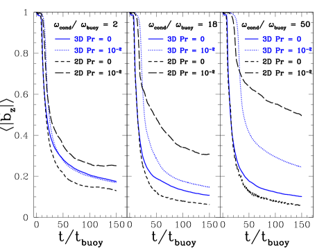
In order to better understand the limitations of 2D simulations, it is useful to compare the 2D and 3D evolution for identical parameters. Figure 4 shows the exact same simulations performed in 2D and 3D for three different conductivities. For the HBI, the results for simulations with different box sizes are essentially the same provided that the same value of is used (McCourt et al., 2011a). We demonstrate this result explicitly in Figure 5 which compares the magnetic geometry evolution for the viscous HBI in two different box sizes. To keep the ratio of fixed, the simulation with has a conductivity and viscosity that are 9 times larger than the simulation with . The evolution, especially at linear and early nonlinear times, is nearly indistinguishable. At very late times, the larger box has experienced slightly more magnetic field evolution as a result of the different modes in the domain relative to the scale height. We conclude from Figure 5 that local simulations of the HBI with are independent of domain size; the results depend instead on the value of , the fundamental dimensionless parameter that quantifies the influence of conduction and viscosity. Thus although the boxes in Figure 4 are only in size, the local simulations with & 50 are quite indicative of how the HBI would evolve on large scales in the ICM (see Fig. 2). The large scales are the most important because both tension and viscosity suppress the growth of the HBI on smaller scales. We justify this interpretation of the local HBI simulations using global cluster models in §6.

Figure 4 shows the mean magnetic field direction, , which is related to the effective vertical thermal conductivity as . In 2D the ability of the HBI to reorient that magnetic field is retarded by viscosity relative to the inviscid case, especially for (right). However, in 3D the effect of the viscosity is much less pronounced. The biggest effect of viscosity is that for , the initial growth of the HBI is slower; however, the instability still produces a significant rearrangement of the magnetic field by . We note that our initial velocity perturbations have white noise amplitudes with a mean magnitude of . For a larger and more realistic perturbation, the linear phase would complete more quickly.
What is the cause of the striking difference in the 2D and 3D evolution of the HBI with viscosity? Recall in Figure 3 that the magnetic field lines strongly bunched up in 2D and could not slip past each other. This type of motion is known as the interchange mode and can be thought of as two magnetic flux tubes slipping past each other. Interchange motions have and therefore are not damped at all by anisotropic viscosity, although they would be damped by an isotropic viscosity. In 3D the magnetic field lines are able to slip past each other, and the HBI is able to continue to reorient the magnetic field. This effect is seen in a different guise in studies of the magnetic Rayleigh-Taylor (RT) instability (Stone & Gardiner, 2007). In 2D, magnetic tension suppresses the RT instability below a critical wavelength; however, in 3D magnetic tension does nothing to suppress the interchange motions of flux tubes. Thus, the instability grows despite the apparent wavelength cut-off in the dispersion relation. This uniquely 3D effect of anisotropic viscosity makes 2D studies of nonlinear saturation irrelevant, and greatly reduces the effect of viscosity relative to what one might naïvely expect from the dispersion relation. It is particularly striking for (right panel in Fig. 4) the non-linear evolution in 3D is quite similar with and without viscosity, although the viscous evolution is delayed by the considerably longer linear growth time.
4.2.2 MTI
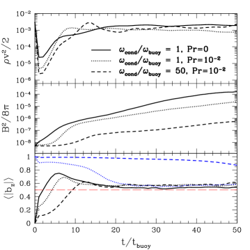
Next, we also examine the nonlinear evolution of the MTI in 3D Cartesian simulations. The dispersion relation shows that the fastest growing modes of the MTI are less affected by viscosity than they are for the HBI. Figure 6 shows the results of our Cartesian simulations of the MTI with and without viscosity and reveals several interesting properties. First, the saturated kinetic energies are largely independent of both the ratio of and whether anisotropic viscosity is included. Note that the simulation with is consistent with the range of clusters in the ACCEPT sample that we have examined (see the right panel of Figure 2). The fact that the kinetic energies are so similar even in the high-viscosity simulation, is likely the result of interchange-like turbulence.
Second, we find the very interesting result that the growth of the magnetic energy (middle panel of Figure 6) is suppressed as the viscosity is increased. This result can be understood in relatively easy terms: the increase in the magnetic field strength in this type of turbulence is proportional to the increase in the length of the magnetic field line, as it is stretched and tangled. These parallel stretching motions are precisely those motions that are damped by anisotropic viscosity, thus suppressing the growth of the magnetic field.
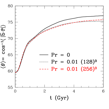
Finally, we consider the reorientation of the magnetic geometry by the MTI (bottom panel of Figure 6). In the inviscid case, an initially horizontal magnetic field is re-oriented to be largely isotropic, in 3D. For modest viscosities , there is little change in the saturated geometry; however, for higher conductivity and viscosities (e.g., ) the magnetic field becomes slightly more vertical than isotropic (about a change in ). We can gain insight into this behavior by considering the evolution of simulations with an initially vertical field, a case that is linearly stable, but non-linearly unstable (see Figure 6 of McCourt et al., 2011a). An initial horizontal perturbation is purely Alfvénic in nature, and thus is unaffected by Braginskii viscosity. A simulation with an initially vertical field and (blue dotted line) evolves towards an isotropic magnetic field configuration. However, in doing so, the field develops a component parallel to the velocity, which is susceptible to viscous damping. Thus, for an initially vertical magnetic field, the higher viscosity simulation (, blue dashed line) evolves much more slowly than its less viscous counterpart. It is precisely this partial stabilization of modes that initially have the field aligned with gravity that results in the radial bias seen in the high-conductivity, horizontal simulation.
5 Global Models of the MTI in Cluster Outskirts
In this section we discuss the effect of Braginskii viscosity on the evolution of the MTI in the outskirts of galaxy clusters using global cluster models. Beyond approximately the scale radius of a cluster, the temperature profile of the ICM almost always declines with radius, thus making it unstable to the MTI. Recent work has shown that the MTI is able to drive large turbulent velocities which provide non-thermal pressure support in hot, massive clusters (Parrish et al., 2011). It is critical to understand this non-thermal pressure support and its implications for measuring cluster masses for use in cosmological parameter estimation through either X-ray or Sunyaev-Zelovich (SZ) methods.
Our initial condition for this section is a spherically-symmetric, hot, massive cluster that resembles Abell 1576 with a mass of . We use a softened NFW profile with a scale radius of kpc and a softening radius of 70 kpc. We initialize an atmosphere in hydrostatic equilibrium using the entropy power law in the ACCEPT database for Abell 1576: a central entropy , , and power-law exponent, (Cavagnolo et al., 2009). If we assume that our fiducial cluster is located at , then for the appropriate WMAP5 cosmological parameters , and the virial radius is Mpc, where corresponds to an overdensity of times the critical density. We do not include cooling, as we focus on the portion of the cluster that is well outside the cooling radius. For full simulation details, see Parrish et al. (2011). By examining Figure 2, we can see that the ratio of in our model is consistent with the range observed in real clusters in the ACCEPT database at the radii of interest ( kpc).
The simulations are carried out on a Cartesian grid in a computational domain that extends from the center of the cluster out to kpc. Within this Cartesian domain, we define a spherical subvolume with a radius of 1225 kpc from which we extract cluster properties. In this volume we initialize tangled magnetic fields with (plasma –) and a Kolmogorov power spectrum. In order to simulate clusters with a negative radial temperature gradient, we fix the temperature at the peak of the cluster temperature profile (approximately 10 keV at 200 kpc) and at the maximum radius (approximately 6.5 keV at 1225 kpc) of our model cluster to the initially-computed temperature values. Thus, we are imposing Dirichlet boundary conditions on the temperature profile. This fixed temperature gradient then drives the continued evolution of the MTI.
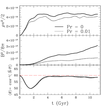

Figure 7 shows the non-linear evolution of the MTI in the global galaxy cluster context. The evolution of the kinetic energy with time is quite similar for both the viscous and inviscid case just as in the local simulations (Figure 6); however, the amplification of the magnetic field is again somewhat suppressed in the viscous case. The magnetic field stretching necessary to amplify the field is exactly the motion that is damped by anisotropic viscosity. This damping of magnetic field amplification makes it more difficult to use a turbulent dynamo, regardless of the source of the turbulence, to amplify the magnetic field from primordial values to those observed today in galaxy clusters. The magnetic geometry evolution is very similar with and without viscosity, as we initially began with a geometrically isotropic magnetic field. A very slight radial bias exists in the steady state in both cases.
Figure 8 shows the saturated and azimuthally-averaged rms Mach number profile for our model cluster at a time of 8.3 Gyr. The turbulence profiles with and without viscosity are almost identical beyond 400 kpc. More quantitatively, at the rms Mach numbers differ by only 5%. Near the very center of the cluster, the rms velocity is actually larger for the viscous simulation. Although we have no definitive explanation, this is perhaps due to the turbulent eddies becoming less aligned with the magnetic geometry. Since our cluster is on the massive and hot end of the cluster mass function, this cluster has a particularly large value of , which yields the greatest effect of viscosity on the linear MTI (see Figure 1). Since viscosity has little effect on the MTI-generated turbulence in this hot cluster, we expect viscosity to make almost no difference for the MTI in lower mass (and cooler) clusters.
6 Global Models of the HBI in Cluster Cores
We now move inwards to consider the effects of viscosity in global models of the cores of galaxy clusters. Within 200 kpc, the cooling times are as short as 100 Myr at kpc. These short cooling times, along with evidence that large mass fluxes of gas are not cooling from a hot to cold phase constitute the modern cooling flow problem (Peterson & Fabian, 2006). Namely, what is keeping cool core cluster cools from cooling further? There has been speculation that thermal conduction from large radii could offset the cooling luminosity (e.g., Narayan & Medvedev, 2001); however, the HBI presents a serious problem to this scenario. Alternatively, there are many observations of AGN feedback that present a more plausible heating mechanism.
The first cluster model we consider is modeled on observations of Abell 2199 (Johnstone et al., 2002). We initialize a cluster in a static NFW halo with a mass of and a scale radius of 390 kpc. In this potential we calculate a spherically-symmetric atmosphere in hydrostatic equilibrium and thermal equilibrium with conduction (at 1/3 of Spitzer) exactly balancing cooling. The model cluster has a central temperature and electron density of keV and , respectively, and a temperature and density of 5 keV and at 200 kpc. This corresponds to a central cooling time of 1.7 Gyr. In this region we initialize a tangled magnetic field with a Kolmogorov power spectrum and an amplitude of . The magnetic field is tangled on scales from 50 kpc down to 30 kpc. The simulations are computed on a Cartesian grid in a domain extending from the cluster center to 240 kpc with gridpoints. A resolution study at showed that the behavior of the magnetic field geometry was almost indistinguishable from the lower resolution results we focus on here (Fig. 9). The magnetic field geometry and temperature profiles as a function of radius (not plotted) are nearly identical; as a result, we consider these simulations very well-converged. In these simulations, the temperature is fixed to the initial temperature at a radius of 200 kpc everywhere, but there is no central boundary condition. For more details of the set-up see Parrish et al. (2009). Our CC atmosphere model has , which is reasonably consistent with the cool-core ACCEPT cluster plotted in Figure 2. Relative to observed clusters, our model is somewhat high in at small radii and on the low-end at larger radii. This discrepancy is due to the fact that by enforcing thermal equilibrium, we demand that conduction match cooling everywhere without any AGN feedback. This is, perhaps, a hint that other heating mechanisms, such as AGN feedback, are necessary for real CC clusters.
We first evolve our fiducial cluster model with anisotropic conduction and cooling only. We diagnose the effect of the HBI by calculating the mean magnetic field angle from radial . This quantity is relevant to the thermal evolution as the effective radial thermal conductivity, often called the Spitzer fraction, is given by
| (23) |
where , which is the radial heat flux if the conduction were purely isotropic at the Spitzer value. Figure 9 shows that the HBI acts to reorient the magnetic field to be more azimuthal, thus reducing the effective radial conductivity. In this calculation the cooling catastrophe (defined as the central temperature reaching our imposed floor of 0.05 keV) occurs at Gyr.
When the effects of Braginskii viscosity are added, the evolution changes very little as shown by the dotted line in Figure 9. As we saw previously in the local calculations, in 3D interchange-type motions are able to proceed unimpeded by any viscosity at all. As the HBI drives rather small turbulent velocities ( at 2 Gyr), the viscous dissipation does next to nothing to impede the cooling catastrophe which occurs at almost the exact same time as in the inviscid simulation. In the Braginskii (collisional, anisotropic) limit, heating by viscous dissipation of turbulence is thermally unstable as , so even more vigorous turbulence cannot stably balance cooling.
Turbulence driven by galaxy wakes, AGN feedback, structure formation, or any other source can counteract the ability of the HBI to reorient magnetic field lines (McCourt et al., 2011a). Quantitatively, turbulence on a scale with velocity is able to suppress the HBI when
| (24) |
where is the HBI growth time, and is a dimensionless constant that is determined by simulations (Sharma et al., 2009; Parrish et al., 2010). Since , this inequality is most difficult to satisfy at the outer scale, which dominates the turbulent energy. Possible sources of turbulence are galaxy wakes (Kim et al., 2005) or AGN feedback itself.

We simulate the interaction of turbulence, the HBI, and cooling in the fiducial cluster core model described previously by adding a random velocity forcing. We drive the velocity fields in Fourier space with a flat spectrum on a scale such that the phases are random and the forcing is incompressible. We have simulated forcing that results in turbulent velocities from 30–, which corresponds to a pressure support of less than a few percent in the cluster cores. The turbulent energy input from this forcing. , is negligible compared to the cooling rate, and thus the turbulence is not energetically important.
Figure 10 shows the late-time, azimuthally-averaged temperature profiles for the same cluster model with different injected turbulent velocities. Viscosity is present at the Spitzer value for these simulations. At low turbulent velocities, , the HBI acts to reorient the magnetic field lines, reducing the effective thermal conductivity and driving the cluster core towards a cooling catastrophe. The time of the cooling catastrophe is reported in parentheses in the legend. Turbulence does indeed delay the cooling catastrophe somewhat, but below a critical value is incapable of preventing it. For example, a turbulent forcing velocity of is able to delay the cooling catastrophe from 2.4 Gyr with no turbulence to 12 Gyr with turbulence.
On the other hand, for larger turbulent velocities, the turbulence is able to keep the magnetic field geometry close to isotropic. In this case, the central temperature approaches a new thermally stable state at a higher temperature. In fact, as increases, the central temperature increases due to both conduction and the larger radially-inward advective heat flux driven by the turbulence. In the final state of the cluster, the central entropy is significantly larger than in the initial condition. For example, a driving velocity of takes the initial central entropy from to .
We find a strikingly strong bimodality in the behavior of the cluster temperature profiles and central entropies. Figure 10 shows that changing the driving velocity by a mere causes a cluster to go from heating approximately balancing cooling () to a core experiencing a cooling castatrophe (). The former simulation is almost exactly on the border of the stability boundary and departs only marginally from the initial temperature profile. This particular case where conduction plus turbulence is balancing cooling to maintain a cool core is an example of fine tuning. For turbulent velocities 5% above or below this value, the core evolves to a clear non-cool-core (NCC) profile or experiences a cooling catastrophe. Note, that we have not included any source of AGN feedback that could avert the cooling catastrophe in the latter situation.
What does Braginskii viscosity do? Including the viscosity makes little difference to the fundamental bimodality observed. In fact, it may even sharpen the transition since the viscosity scales as . A cluster whose core is heating from the initial condition becomes more viscous and thus a given turbulent velocity is more readily able to reorient the magnetic field relative to the HBI as the temperature increases.
We checked the robustness of our conclusions by varying our initial fiducial physical a variety of ways:
-
•
A hotter, more massive CC cluster. We initialize a model with a central temperature of 2.5 keV and entropy of which increases to a temperature of 8 keV at 300 kpc. In the absence of turbulence this cluster proceeds to a cooling catastrophe in Gyr, much as our fiducial model. With turbulent driving at an rms velocity of , the cluster transitions to a NCC cluster with a central entropy of . The viscous and inviscid cases are very similar as in our fiducial calculation.
-
•
A NCC cluster of equivalent mass. We initialize our fiducial model with temperature ranging from 4 keV to 5 keV over 200 kpc and a central entropy of . From linear theory, one expects viscosity to reduce the HBI growth rates somewhat due to the higher ratio of relative to our fiducial model (see Figure 1); however, the evolution of the temperature profile is almost indistinguishable with and without viscosity. Without any imposed turbulence this cluster reaches a cooling catastrophe around 6.2 Gyr which is somewhat faster than the initially predicted cooling time of 7.2 Gyr.333This cooling time is an overestimate as the Bremsstrahlung cooling rate increases as material cools at constant pressure.
-
•
A hotter, more massive NCC cluster We initialize a hotter cluster with a mass of and a temperature that ranges from 6 keV at the center to 8 keV at 300 kpc. This model has a scale radius of 650 kpc and a central entropy of . The profile of is shown in Figure 2 with the NCC (HBI) label. The value of is at 50 kpc and at 100 kpc, consistent with the ACCEPT NCC measurements. Figure 11 shows the evolution of the radial profile of the magnetic field angle from its initial statistical isotropy of . In the majority of the volume, the magnetic field is reoriented to be substantially more tangential () with little difference between the viscous and inviscid cases. The small radial bias around 20 kpc is caused by inhomogeneous radial infall as the cluster begins to suffer a cooling catastrophe. Based on the profiles in Figure 2, viscosity is even more important at these small radii in the initial cluster model; additional suppression of the HBI may be present but is overwhelmed by the effects of cooling in our global calculations. At larger radii, viscous effects are smaller, and the HBI has already reduced conduction from the outskirts. Overall this hot, NCC cluster model shows that the HBI can operate even when viscous effects are important.
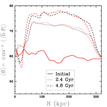
Figure 11: Radial profiles of the azimuthally-averaged angle of the magnetic field with respect to the radial direction in our global non-cool-core cluster model (model NCC in Fig. 2) at two times. is radial. corresponds to a random, isotropic magnetic field. The HBI reorients the magnetic field, reducing the effective conductivity, which precipitates the cooling catastrophe at 2.4 Gyr. Very little difference is seen between the inviscid (black curves) and viscous (red curves) evolution. The radial bias seen around 20 kpc is due to inhomogeneous radial infall. -
•
Reduced magnetic field correlation length. We simulate our fiducial cluster with the magnetic field tangled on scales ranging from 20 kpc to 10 kpc. The shorter correlation length can reduce the effective conduction length scale, increasing , and reducing the HBI growth rate. The thermal evolution, however, is nearly identical to our fiducial model both with and without viscosity.
-
•
Higher initial magnetic field. We simulate our fiducial cluster with the magnetic field increased to which is similar to observed magnetic field strengths (Carilli & Taylor, 2002). Magnetic tension is able to suppress short wavelength modes in a way very similar to viscosity. With the higher field, the HBI proceeds slightly more slowly and the fiducial cluster reaches a cooling catastrophe approximately 200 Myr later. We find no difference between the viscous and inviscid simulations.
7 Discussion and Conclusions
The dilute plasma in the ICM of galaxy clusters has a mean free path along magnetic field lines that is many orders of magnitude larger than the electron/proton gyroradii. As a result, thermal conduction by electrons and momentum transport by ions are strongly anisotropic with respect to the magnetic field. In this paper we have carried out the first simulations of buoyancy instabilities in the ICM (the MTI and HBI) that include anisotropic conduction and viscosity simultaneously and self-consistently. This extends the analytic work of K11, who showed that viscosity can change the instabilities in the limit of very rapid conduction/viscosity, suppressing the growth rates of some of the modes (Fig. 1).
In 2D simulations of the HBI, viscosity changes the nonlinear saturation of the instability. Figure 3 shows that strong viscosity drives the magnetic field to bunch up in prominent vertical structures. However, in 3D the magnetic field lines slip past each other in interchange-like motions. These interchange motions are not damped by parallel viscosity. As a result, in 3D the saturated state of the HBI (as measured by statistical quantities like ) is not as strongly altered by the addition of viscosity, although it can take longer to reach the saturated state because viscosity slows the growth of the modes (Figure 4). This conclusion is true even for very rapid conduction (and thus very rapid viscous damping), with (where the conduction frequency here is defined across the scale of the box ); this is a value characteristic of cluster cores (Fig. 2).
In the cores of galaxy clusters the cooling times are short compared to the age of the universe. There is a long-standing problem of finding processes that can provide sufficient heating to counteract this cooling. One possible solution is for conduction to bring in heat from the large thermal reservoir beyond the core. However, in the absence of other sources of turbulence, the HBI exacerbates the cooling flow problem by reorienting magnetic field lines to be more azimuthal, thus reducing the effective radial thermal conductivity, . Our global simulations of realistic cool-core cluster models (Fig. 2) demonstrate that this reorientation of the magnetic geometry by the HBI is only minimally influenced by anisotropic viscosity (Fig. 9 & 11).
We also simulated galaxy cluster cores with additional turbulent forcing, intended to mimic the turbulence driven by galaxy wakes and/or AGN feedback. Turbulence is capable of suppressing the magnetic field reorientation of the HBI when the eddy turnover time is similar to the instability growth time (see Figure 11 of McCourt et al., 2011a). The interplay between turbulence, the HBI, and cooling in the cluster core, results in a very strong bimodality in the temperature profile and other cluster properties such as the central entropy (Parrish et al., 2010). Modest levels of subsonic turbulence, less than , are capable of transforming a cool core cluster into a non-cool-core cluster. This turbulence is energetically small compared to the cooling luminosity in the cluster core; instead, the turbulence can be considered a catalyst that enables conduction to efficiently couple to the central regions. Larger turbulent velocities result in larger central temperatures and entropies, aided by both conduction and an inwardly-directed turbulent heat transport. With Braginskii viscosity, these conclusions about cluster bimodality are unchanged. In fact, we believe that viscosity aids the generation of a bimodal cluster population: as the cluster core heats up, it becomes more viscous, which makes it somewhat more difficult for the HBI to re-orient the magnetic field, further promoting the transition to a non-cool-core cluster.
Our numerical experiments are encouragingly consistent with the observed bimodality in cluster core properties (Voit et al., 2008; Cavagnolo et al., 2009). We find that cool-core clusters (with central entropies ) cannot be efficiently heated by conduction and must have an additional source of heating. This source is plausibly AGN feedback through bubbles, jets, or other coupling mechanisms. Indeed, cool-core clusters generically show evidence of radio emission consistent with AGN activity. With turbulence above a critical threshold value, however, we find that conduction is able to transform a cool-core cluster into a non-cool-core cluster with a much higher central entropy—this does not necessarily require AGN activity though it does require roughly volume-filling turbulence. Observationally, this is consistent with the lack of significant AGN feedback indicators for high central entropy clusters.
In local Cartesian simulations of the MTI we find that the evolution of kinetic energy is statistically unchanged by anisotropic viscosity; however, the amplification of the magnetic field is diminished with the addition of viscosity (Fig. 6). Magnetic fields are amplified by turbulence increasing the length of magnetic field lines; this motion is precisely the one damped by anisotropic viscosity. As a result, the magnetic field is amplified more slowly than the kinetic energy with anisotropic viscosity. For simulations with initially horizontal fields, increased viscosity leads to a small vertical bias in the magnetic field direction relative to isotropy. Simulations that start with initially vertically magnetic fields, a nonlinearly unstable configuration, evolve much more slowly at high viscosity (bottom panel of Fig. 6). This mechanism explains the small vertical bias seen for higher viscosity.
In the outskirts of galaxy clusters, the temperature declines with increasing radius and the plasma is unstable to the MTI rather than the HBI. At these radii, the MTI can generate significant turbulent velocities up to an rms Mach number of near . This turbulence represents a non-thermal source of pressure that can bias hydrostatic estimates of cluster masses. As emphasized in Parrish et al. (2011), this turbulence is in addition to that generated by structure formation. In the global cluster models of the MTI presented here (Fig. 8), we find that viscosity only weakly affects this turbulence, as predicted analytically by K11. The rms velocities with viscosity are only 5% smaller than the inviscid case. Consistent with our local simulations, we find that the amplification of the magnetic field is modestly reduced for simulations with viscosity. The fact that anisotropic viscosity specifically damps all sources of turbulence that couple to magnetic field amplification makes it more difficult to invoke turbulent mechanisms for amplifying the magnetic field in clusters from primordial values.
Although our results with anisotropic viscosity do not significantly change any of the previous conclusions about the role of the HBI and MTI in the ICM, we believe that it is important to have established this conclusively. Most importantly, a fluid with a low collisionality like the ICM or the solar wind has a high viscosity, as the viscosity scales inversely with the collision frequency; the Reynolds number is correspondingly rather small (Fig. 2). Thus the importance of viscosity is not a priori clear and needed to be explicitly studied. In future work it will be interesting to consider the role of anisotropic viscosity on other problems in the ICM, such as cold fronts or the large surface brightness fluctuations (ripples) observed in Perseus (Fabian et al., 2006).
Appendix A Algorithm and Tests of Anisotropic Viscosity
A.1 Method
We now describe the details of our algorithm for anisotropic momentum transport. This algorithm is similar to that used in Dong & Stone (2009). For simplicity consider the momentum and energy equations with only anisotropic viscosity
| (25) | |||||
| (26) |
where the viscous stress tensor is given by Equation 9. We proceed to discretize this in a very similar manner to how anisotropic conduction was first discretized in Parrish & Stone (2005). For example, the first component in square brackets of the tensor has terms that can be written as
| (27) |
where the ellipsis indicates similar derivatives of and , respectively. We will see momentarily that this stress is computed as an area-averaged, face-centered quantity which then requires velocity derivatives to be appropriately centered.
The calculation of is straightforwardly discretized from the cell-centered velocities. The calculation of the transverse velocity gradients, such as requires special care as monotonicity is required. This issue surfaces in anisotropic thermal conduction when it proves essential to limit the slope of the transverse temperature derivatives, e.g. the term in the calculation of , to prevent heat from being conducted from cold to hot regions (Sharma & Hammett, 2007).
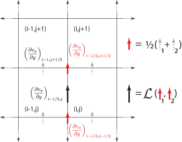
This type of non-monotonicity can lead to negative internal energies with conduction. The same symptom can occur with viscosity, and it is necessary to ensure that momentum flows in the correct direction at all times. We therefore interpolate the transverse velocity gradients to cell faces with a slope limiter:
| (28) |
where represents the left face of cell (), and represents a slope limiter. The velocity gradients at cell edges are simply arithmetic averages, e.g.
| (29) |
We choose the monotonized central difference (MC) limiter for our slope limiter (see van Leer, 1979, for details).
Our explicit methods for anisotropic conduction and viscosity both have timesteps that are more restrictive than the MHD timestep as they are parabolic equations. The momentum diffusion has a Courant-limited timestep that is proportional to . Therefore, we choose to sub-cycle both diffusive operators with respect to the MHD timestep. For the anisotropic viscosity, we are able to simply call the standard MHD boundary conditions in between each sub-cycle. Due to the smaller physical diffusivity, we are able to take much longer timesteps for viscosity than conduction. Sub-cycling the conduction and viscosity do not change the evolution of the HBI compared to reducing the MHD timestep to match the conduction timestep.
After these preliminaries, we are now prepared to outline the method for anisotropic momentum transport. Careful attention is paid to the centering of the terms in the difference equations. Our method resembles the underlying Godunov scheme for Athena in that conservative cell-centered variables, e.g. momentum, are updated by differencing face-centered fluxes, e.g. the viscous stress—such a scheme is manifestly conservative. Our method for calculating one sub-cycle of a cell centered on () is as follows:
-
1.
Apply the MHD boundary conditions to synchronize all ghost zones across processors.
-
2.
Calculate face-centered velocity gradients, including limiters on transverse gradients, e.g. .
-
3.
Calculate the face-centered viscous prefactor
(30) where the diffusion coefficient (sometimes known as the kinematic viscosity) depends on density and temperature as . The density dependence drops out of the stress tensor. The density dependence, however, is relevant for calculation of the viscous timestep.
-
4.
Calculate the face-centered viscous stresses, e.g. on the left -face.
-
5.
Difference the viscous stresses to get a cell-centered update to the energy and momentum equation, which is in the -direction:
(31) (32) There are similar terms in the - and -directions. The here is the sub-cycle timestep.
Steps (i)–(v) are repeated for each sub-cycle.
A.2 Verification
It is important to verify a new numerical method, such as anisotropic viscosity, with test problems with known solutions. To wit, we begin with two tests of the physics of linear MHD waves. We take advantage of the property that Braginskii viscosity damps viscous motions only along field lines; however, our numerical implementation will have some spurious .
We test our algorithm by measuring the viscous damping rates of MHD waves. These damping rates are sensitive to both the magnitude and anisotropy of the viscosity and therefore provide a stringent test of our code. Moreover, when the viscosity is small enough (quantified later), the damping rates can be calculated analytically, permitting a rigorous point of comparison for our simulations. In order to test the multi-dimensional nature of the code, we pick the wave vector to be 45∘ from the grid axes and the magnetic field to be 56.3∘ from . Thus, nothing is aligned with the grid axes and all terms in our algorithm are evaluated.
Alfvén waves directly probe the anisotropy of our algorithm. The fluid motions induced by these waves are purely transverse to the magnetic field and therefore are not damped by parallel viscosity. Any measured damping represents a spurious perpendicular (or isotropic) viscosity due to errors in the algorithm. We confirm that our code does not damp Alfvén waves: even with an extremely large viscosity , where is the wavelength and is the wave period, we measure a damping rate of . This damping is only % larger than that produced by the inviscid, default version of Athena with no explicit viscosity. For more reasonable viscosities, this damping is much reduced. Thus, the spurious, cross-field diffusion in our algorithm is typically much smaller than other sources of numerical dissipation in our simulations.
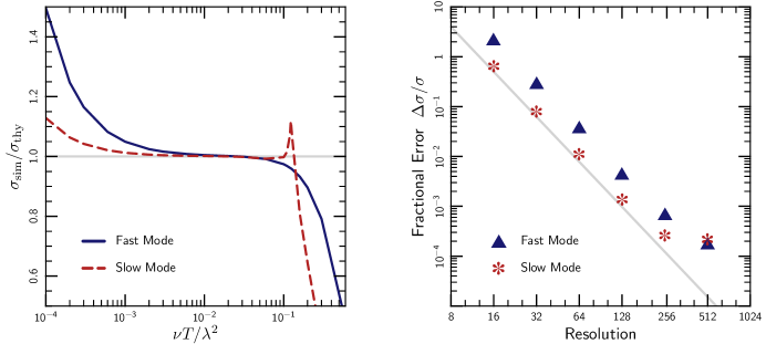
We test the parallel component of the viscosity by measuring the damping of fast and slow magnetosonic waves. Both of these waves have a component of velocity parallel to the magnetic field and thus damp at a rate
| (33) |
where , , and are unit vectors in the directions of the magnetic field, wave vector, and wave perturbation velocity, respectively (Braginskii, 1965). Figure 13 compares the damping rates measured in our simulations with this analytic expectation. In the left panel, we plot the ratio of the measured to expected damping rates. The disagreement at low viscosities is most likely caused by the numerical, isotropic viscosity inherent in Athena’s integrator. This viscosity is not included in the analytic expectation, so equation 33 underestimates the damping rate in this limit. With higher viscosity , the linear damping assumption in the derivation of equation 33 is not valid. The algorithm performs well in between these limits.
In order to test the the numerical convergence of our algorithm, we chose a fiducial viscosity , such that the damping remains small but is not dominated by numerical viscosity. We plot the fractional error in the damping rate in the right panel of Figure 13. This is not the usual L2 norm that is often plotted for linear wave convergence tests. Even at 16 zones/wavelength, the damping rate is correct to order unity. The quantity converges at third order. This excellent convergence results from a convolution of the increasing accuracy of the linear waves themselves as well as the improved accuracy of the viscous transport, both of which are second-order algorithms.
Perhaps the most demanding test of our combined algorithm for MHD, anisotropic conduction, and anisotropic viscosity is our measurement of the linear growth rates of the HBI and MTI in Figure 1. We are able to confirm the analytic growth rates to within %, but unfortunately cannot reach the same accuracy as with the linear MHD waves.
At least two effects limit our precision when measuring the growth rates of the HBI and MTI. First, the analytic growth rates to which we compare are only strictly known in the WKB limit . Practical considerations limit our simulation setups to , however. We expect corrections to the analytic growth rates of order , similar the typical discrepancy in our measurements. Additionally, the structure of the eigenmodes of the HBI and MTI depend on the growth rate. Since we only know the growth rate to an accuracy of %, we cannot initialize the simulation in an exact eigenstate. Thus, the perturbations we apply do not grow strictly exponentially in our simulations; there is an initial period of order during which the perturbations settle into their respective eigenstates. In practice, this limits the period of growth from , when exponential growth begins, to , when the instability begins to become nonlinear. Thus we have only a limited time window over which to fit the data and cannot reach an arbitrary level of precision. It might seem that we could delay saturation, and therefore improve the accuracy of our growth rate measurement, by using a smaller initial perturbation. In practice, however, our boundary conditions do not hold hydrostatic equilibrium perfectly and eventually generate motions of order . Thus, when we use a weaker perturbation we lose it in the noise.
Despite these limitations, we are able to confirm the growth rates with a comparable accuracy to the validity of the analytic theory. This, along with our measurements of the damping of linear MHD waves, represents a strong validation of our code.
Acknowledgments
We thank Jim Stone for sharing the anisotropic viscosity module used in Dong & Stone (2009) with us and for useful feedback on the paper. We also thank Matt Kunz for helpful comments on an early draft. Support was provided in part by NASA Grant ATP09-0125, NSF-DOE Grant PHY-0812811, and by the David and Lucille Parker Foundation. Support for P.S. was provided by NASA through the Chandra Postdoctoral Fellowship grant PF8-90054 awarded by the Chandra X-Ray Center, which is operated by the Smithsonian Astrophysical Observatory for NASA under contract NAS8-03060. We would like to thank the hospitality of the KITP where much of this work was performed and supported in part by the National Science Foundation under grant PHY05-51164. The computations for this paper were perfomed on the Henyey cluster at UC Berkeley, supported by NSF grant AST-0905801 and through computational time provided by the National Science Foundation through the Teragrid resources located at the National Institute for Computational Sciences under grant TG-AST080049.
References
- Balbus (2000) Balbus, S. A. 2000, ApJ, 534, 420
- Bogdanović et al. (2009) Bogdanović, T., Reynolds, C. S., Balbus, S. A., & Parrish, I. J. 2009, ApJ, 704, 211
- Braginskii (1965) Braginskii, S. I. 1965, Reviews of Plasma Physics, ed. M. A. Leontovich, Vol. 1 (New York: Consultants Bureau), 205
- Carilli & Taylor (2002) Carilli, C. L., & Taylor, G. B. 2002, ARA&A, 40, 319
- Cavagnolo et al. (2009) Cavagnolo, K. W., Donahue, M., Voit, G. M., & Sun, M. 2009, ApJS, 182, 12
- Dong & Stone (2009) Dong, R., & Stone, J. M. 2009, ApJ, 704, 1309
- Fabian et al. (2006) Fabian, A. C., Sanders, J. S., Taylor, G. B., Allen, S. W., Crawford, C. S., Johnstone, R. M., & Iwasawa, K. 2006, MNRAS, 366, 417
- Gardiner & Stone (2008) Gardiner, T. A., & Stone, J. M. 2008, Journal of Computational Physics, 227, 4123
- Johnstone et al. (2002) Johnstone, R. M., Allen, S. W., Fabian, A. C., & Sanders, J. S. 2002, MNRAS, 336, 299
- Kim et al. (2005) Kim, W., El-Zant, A. A., & Kamionkowski, M. 2005, ApJ, 632, 157
- Kunz (2011) Kunz, M. W. 2011, MNRAS, 1288
- McCourt et al. (2011a) McCourt, M., Parrish, I. J., Sharma, P., & Quataert, E. 2011a, MNRAS, 413, 1295
- McCourt et al. (2011b) McCourt, M., Sharma, P., Quataert, E., & Parrish, I. J. 2011b, ArXiv:1105.2563
- Narayan & Medvedev (2001) Narayan, R., & Medvedev, M. V. 2001, ApJL, 562, L129
- Parrish et al. (2011) Parrish, I. J., McCourt, M., Quataert, E., & Sharma, P. 2011, MNRAS, L356
- Parrish & Quataert (2008) Parrish, I. J., & Quataert, E. 2008, ApJL, 677, L9
- Parrish et al. (2009) Parrish, I. J., Quataert, E., & Sharma, P. 2009, ApJ, 703, 96
- Parrish et al. (2010) —. 2010, ApJL, 712, L194
- Parrish & Stone (2005) Parrish, I. J., & Stone, J. M. 2005, ApJ, 633, 334
- Parrish & Stone (2007) —. 2007, ApJ, 664, 135
- Peterson & Fabian (2006) Peterson, J. R., & Fabian, A. C. 2006, PhysRep, 427, 1
- Quataert (2008) Quataert, E. 2008, ApJ, 673, 758
- Reynolds et al. (2005) Reynolds, C. S., McKernan, B., Fabian, A. C., Stone, J. M., & Vernaleo, J. C. 2005, MNRAS, 357, 242
- Ruszkowski & Oh (2010) Ruszkowski, M., & Oh, S. P. 2010, ApJ, 713, 1332
- Sharma et al. (2009) Sharma, P., Chandran, B. D. G., Quataert, E., & Parrish, I. J. 2009, ApJ, 699, 348
- Sharma & Hammett (2007) Sharma, P., & Hammett, G. W. 2007, Journal of Computational Physics, 227, 123
- Spitzer (1962) Spitzer, L. 1962, Physics of Fully Ionized Gases (Physics of Fully Ionized Gases, New York: Interscience (2nd edition), 1962)
- Stone & Gardiner (2007) Stone, J. M., & Gardiner, T. 2007, ApJ, 671, 1726
- Stone et al. (2008) Stone, J. M., Gardiner, T. A., Teuben, P., Hawley, J. F., & Simon, J. B. 2008, ApJS, 178, 137
- Tozzi & Norman (2001) Tozzi, P., & Norman, C. 2001, ApJ, 546, 63
- van Leer (1979) van Leer, B. 1979, Journal of Computational Physics, 32, 101
- Voit et al. (2008) Voit, G. M., Cavagnolo, K. W., Donahue, M., Rafferty, D. A., McNamara, B. R., & Nulsen, P. E. J. 2008, ApJL, 681, L5