RELATIVISTIC MODEL ON PULSAR RADIO EMISSION AND POLARIZATION

Abstract

We have developed a relativistic model for pulsar radio emission and polarization by taking into account of detailed geometry of emission region, rotation and modulation. The sparks activity on the polar cap leads to plasma columns in the emission region and modulated emission. By considering relativistic plasma bunches streaming out along the rotating dipolar field lines as source of curvature radiation, deduced the polarization state of the radiation field in terms of the Stokes parameters. We have simulated a set of typical pulse profiles, and analyzed the role of viewing geometry, rotation and modulation on the pulsar polarization profiles. Our simulations explain most of the diverse behaviors of polarization generally found in pulsar radio profiles. We show that both the ‘antisymmetric’ and ‘symmetric’ types of circular polarization are possible within the frame work of curvature radiation. We also show that the ‘kinky’ nature in the polarization position angle traverses might be due to the rotation and modulation effects. The phase lag of polarization position angle inflection point relative to the phase of core peak also depends up on the rotationally induced asymmetry in the curvature of source trajectory and modulation.

1 INTRODUCTION

Even though pulsars were discovered more than four decades ago, their radio emission process is still not completely understood. The very high degree of linear polarization and systematic polarization position angle (PPA) swing of pulsar radiation have been naturally invoked in curvature radiation (Sturrock, 1971; Ruderman & Sutherland, 1975). In the frame work of curvature radiation models the radio emission is believed to be emitted by relativistic plasma streaming ‘force-freely’ along the open field lines of the super-strong magnetic field, the geometry of which is assumed to be predominantly dipolar. In the non-rotating approximation, the velocity of relativistic plasma will be parallel to the tangents of the field lines to which they are associated with, and hence emitted radiation beamed in the direction of field line tangents. In the rotating vector model (RVM), as the pulsar rotates, observer sight line encounters different dipolar field lines, and results in the ‘S’ shaped PPA swing, which is more or less determined by the geometry of emission region (Radhakrishnan & Cooke, 1969; Komesaroff, 1970).

Pulsar radio emission is believed to be coming from mainly open dipolar field lines which lie within the polar cap region. The shapes of individual pulses indicate that the entire polar cap might not be radiating uniformly. The sub-pulse modulation can be explained on the idea of isolated sparks on the polar cap (e.g., Ruderman & Sutherland, 1975; Cheng & Ruderman, 1980). Pulsar average profiles resulted from the summation of several hundreds of individual pulses, have well defined shapes and in general they made up of many components. Phenomenologically, pulsar emission is recognized as central ‘core’ emission arising from the region near to the magnetic pole and ‘cone’ emission arising from concentric rings around the pole (e.g., Rankin, 1983, 1990, 1993; Mitra & Deshpande, 1999; Gangadhara & Gupta, 2001; Mitra & Rankin, 2002). However, there are some contrary arguments that the emission is ‘patchy’ (Lyne & Manchester, 1988).

Since pulsars are fast spinning objects, the rotation effects such as aberration, retardation and polar cap currents are believed to be strongly influencing their emission. For an inertial observer, in addition to intrinsic velocity along the field line tangents, particles will have co-rotation velocity component. Therefore, in the inertial observer frame, the net velocity of particles will be offset from the field line tangents to which they are associated with, and hence the emission will be aberrated in the direction of pulsar rotation. By taking into account of rotation, Blaskiewicz, Cordes and Wasserman (1991), hereafter BCW (1991), have proposed a relativistic pulsar polarization model. By assuming a constant emission altitude $r$ across the whole pulse, they have predicted that the midpoint of the intensity profile shifts to the earlier phase by $\sim r/r_{LC}$ with respect to fiducial phase, whereas PPA inflection point shifts to later phase by $\sim 3r/r_{LC}.$ The parameter $r_{LC}=c~{}P/2\pi$ is the light cylinder radius, and $c$ is the velocity of light and $P$ is the pulsar rotation period. Further, they have shown that the intensity on leading side becomes stronger than that on trailing side due to rotation, which has strong observational support (Lyne & Manchester, 1988). Hibschman & Arons (2001) further improved the relativistic RVM model by taking into account of induced magnetic field due to polar cap currents. Dyks (2008) has presented a more simple derivation in which he has reproduced the BCW (1991) prediction. Following these deductions Thomas & Gangadhara (2010) have estimated the absolute emission altitudes of a few pulsars. The asymmetry in the phase location of conal components with respect to core has been interpreted in terms of rotation effects such as aberration and retardation phase shifts (Gangadhara & Gupta, 2001; Gupta & Gangadhara, 2003; Dyks, Rudak & Harding, 2004; Gangadhara, 2005; Krzeszowski et al., 2009).

By solving the equation of motion, Thomas & Gangadhara (2007) have also predicted that the emissions on leading side dominate over the trailing side due to rotation induced asymmetry in the curvature of trajectory of bunches. Dyks, Wright & Demorest (2010) have analyzed the influence of rotation on shape of pulse profiles of millisecond pulsars and identified two opposing effects of corotation: (1) the caustic enhancement of the trailing side emission due to squeezing into a narrower component; and (2) the weakening of the trailing side caused by the the smaller curvature of source trajectories. Thomas, Gupta & Gangadhara (2010) have discussed the significance of geometric and rotation effects on the pulsar radio profiles and interpreted the asymmetry in the pulsar radio profiles, particularly “partial cones” (which were first termed by Lyne & Manchester, 1988) in terms of the rotation effects. These are notable for their highly asymmetric average intensity profiles and PPA traverses, wherein one side of a double component conal profiles is either missing or significantly suppressed, and the PPA inflection point lies well towards the trailing side.

Among the several theoretical problems related to exploring the pulsar radio emission mechanism, the mostly unexplained observational fact is the high degree of circular polarization and its very diverse behavior. By analyzing average pulsar profiles, Radhakrishnan & Rankin (1990) have identified two types of circular polarization, namely, ‘antisymmetric’, where the circular polarization changes its sense near the center of the pulse profile, and ‘symmetric’, where the circular polarization will have the same sense across the whole pulse profile. In the case of pulsars with antisymmetric type, they found a strong correlation between the sense reversal of circular polarization and the PPA swing, and speculated that it could be a geometric property of emission mechanism. Han et al. (1998) have noticed that the circular polarization is common in pulsars but diverse in nature, and even though it is generally strongest in the central or ‘core’ regions, is by no means confined to central regions. They found a strong correlation between the sense of circular polarization and the PPA swing in the double-conal pulsars, and no correlation between the sense reversal of circular polarization near the center of pulse profiles and the PPA swing in the pulsars with antisymmetric type of circular polarization. Further, You & Han (2006) have reconfirmed these investigations with a larger data.

There are two probable origins of circular polarization proposed for the pulsar radiation: either intrinsic to the emission mechanism (e.g., Michel, 1987; Gil & Snakowski, 1990a, b; Radhakrishnan & Rankin, 1990; Gangadhara, 1997, 2010) or generated by the propagation effects (e.g., Cheng & Ruderman, 1979; Melrose, 2003). Gil, Kijak & Zycki (1993) have modeled the single-pulse polarization characteristics of pulsar radiation and argued that the strong sense reversing circular polarization is a natural feature of curvature radiation. Cheng & Ruderman (1979) have suggested that conversion of linear polarization to circular polarization is possible due to expected asymmetry between the positive and negative charged components of magneto active plasma in the far magnetosphere. On the other hand, Kazbegi, Machabeli & Melikidze (1991) have argued that the cyclotron instability, rather than propagation effect, is responsible for the circular polarization of pulsar radiation. By considering the rotation of magnetosphere, Lyubarskii & Petrova (1999) have shown that the induced wave mode coupling in the polarization-limiting region can result in circular polarization in linearly polarized normal waves. Melrose (2003) reviewed the properties of intrinsic circular polarization, and the circular polarization due to cyclotron instability, and discussed the circular polarization due to propagation effects in an inhomogeneous birefringent plasma.

Recently, Gangadhara (2010) has developed a curvature radiation model by considering the detailed geometry of emission region in the non-rotating pulsar approximation. His results supports the fact that the circular polarization survives only when there is a sufficient gradient in the sub-pulse modulation, and the antisymmetric circular polarization is an intrinsic nature of the curvature radiation. He has confirmed the Radhakrishnan & Rankin (1990) correlation between the sense reversal of circular polarization and the PPA swing. He has also shown that the sense reversal of circular polarization is by no means confined to central core regions.

Although an extensive pulsar polarimetric studies are available, the pulsar emission and polarization are not well understood due to their diverse nature. Despite the rotation effects such as aberration and retardation are strongly believed to influence the pulsar radio profiles, a complete polarization model including rotation effects has not been attempted in the literature. In the work of Thomas and co-authors, and Dyks, Wright & Demorest (2010) modeled only the total intensity, and left the polarization part untouched. On the other hand, relativistic models proposed by BCW (1991), Hibschman & Arons (2001), and Dyks (2008) deals with PPA only, and not even the linear polarization. Further, in their models, emission from the points at which bunch velocity exactly aligns with the sight line is only considered, and the emissions from the neighboring points at which velocity lies within $\sim 1/\gamma$ with respect to sight line are not considered. But such emissions does have influences on PPA swing if modulated as we show in our model.

For the first time, we have developed a complete polarization model by taking into account of a detailed geometry of emission region, rotation effects and modulation. We adopt the features of curvature radiation, and incorporated the Gaussian sub-pulse modulation. At any instant of time, observer tends to receive the incoherent curvature radiation from a modulated beaming region, which constitutes a small flux tube of dipolar field lines. Based on simulated profiles, we discuss the combined effect of rotation and modulation on the typical pulsar radio profiles. We ascribe the asymmetry in the pulsar radio profiles in terms of combined effects of viewing geometry, rotation, and modulation. In § 2 we derive the expressions for radiation electric field in frequency domain and the Stokes parameters. In § 3 we present the simulation of typical pulse profiles, and the discussion in § 4 and conclusion in § 5.

2 POLARIZATION STATE OF THE RADIATION FIELD

Relativistic plasma streaming ‘force-freely’ along the super-strong dipolar magnetic field lines emit beamed curvature radiation. The curvature radiation model requires an efficient plasma bunching to account for the very high brightness temperature of the pulsar radio emission, wherein the plasma bunches of size less than or equal to the radiation wavelength can emit coherently (e.g., Sturrock, 1971; Ruderman & Sutherland, 1975; Cheng & Ruderman, 1980). In our model, we treat the plasma bunch as a single particle of charge $q=Ne,$ where $e$ is the electronic charge, and $N$ is the number of particles. In this paper we alternatively use source, particle, or plasma bunch as source of radio emission but they all mean the same. The emissions from different bunches become incoherent as such emissions do not bear any phase relation.

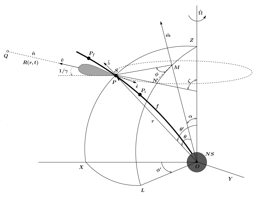
Figure 1: Geometry of radiation emission from a relativistic source S accelerated along a rotating field line f (thick curve) in a stationary inertial frame XYZ with neutron star center O as the origin. $\hat{\Omega}$ is the rotation axis, $\hat{m}$ is the magnetic axis, and $\hat{b}$ is the field line tangent. The rotation direction is $\hat{\epsilon}$ and the net velocity is $\hat{v}$. The observer’s sight line $\hat{n}$ lies in the fiducial plane (XZ-plane). ZPX, ZML, and XL are the great circles centered on O. The observation point Q is at a distance R from the emission point P.

Consider an inclined and rotating magnetic dipole in the inertial observer’s frame (IOF), a stationary Cartesian coordinate system–XYZ with neutron star center O as the origin as shown in Figure 1. The angular velocity $\Omega$ is considered along positive Z-axis, and the magnetic axis $\hat{m}$ is inclined by an angle $\alpha$ with respect to $\Omega$. Consider a radiation source S constrained to move along the rotating field line f. The velocity v of the source is given by

$$\textbf{v}=\kappa c\,\hat{b}+\mathbf{\Omega}\times\textbf{r}~{},$$ (1)

where $\hat{b}$ is unit tangent vector to the field line and r is the position vector of the source, and their expressions are given in Gangadhara (2010). The parameter $\kappa$ specifies the speed of the source along the field line as a fraction of the speed of light c. The first term on the r.h.s. of Equation (1) is the velocity in the corotating frame and is in the direction of the associated field line tangent, and the second term is corotation velocity. Hence the velocity of the source is offset from the field line tangent to which it is associated with, and is aberrated in the direction of pulsar rotation. The parameter $\kappa$ can be deduced from the Equation (1) by assuming $|\textbf{v}|=\beta c$,

$$\kappa=\sqrt{\beta^{2}-\left(\frac{\Omega r}{c}\right)^{2}\sin^{2}\theta^{\prime}\sin^{2}\Theta}-\frac{\Omega r}{c}\sin\theta^{\prime}\cos\Theta~{},$$ (2)

where $\beta=\sqrt{1-1/\gamma^{2}}$, $\gamma$ is the Lorentz factor of the source, $\theta^{\prime}$ is the angle between r and $\Omega$, and $\Theta$ is the angle between b and the rotation direction $\hat{\epsilon}$. The expressions for $\theta^{\prime}$ and $\Theta$ are given in Gangadhara (2005).

The acceleration $\textbf{a}=d\textbf{v}/dt$ of source in IOF is given by

$$\textbf{a}=\frac{(\kappa c)^{2}}{|\textbf{b}|}\frac{\partial\hat{b}}{\partial\theta}+\frac{\kappa c^{2}}{|\textbf{b}|}\frac{\partial\kappa}{\partial\theta}\hat{b}+2\kappa c(\mbox{\boldmath$\Omega$}\times\hat{b})+\mbox{\boldmath$\Omega$}\times(\mbox{\boldmath$\Omega$}\times\textbf{r})~{},$$ (3)

where we have used the expression of arc length of the field line $ds=|\textbf{b}|d\theta=\kappa c~{}dt$ wherein $|\textbf{b}|$ is the magnitude of the field line tangent and $\theta$ is magnetic colatitude. The expression for $|\textbf{b}|$ is given in Gangadhara (2004).

The first term on r.h.s. of Equation (3) is the acceleration of bunch due to curvature of dipolar magnetic field line, and this is the only term which exists in the absence of rotation (Gangadhara, 2010). The second term is due to a small change in the speed of bunch due to motion along field line. The third and last terms are the accelerations due to Coriolis and the Centrifugal forces, respectively.

As the relativistic source accelerates along the rotating field line, it emits curvature radiation whose spectral distribution at the observation point Q is given by (Gangadhara, 2010)

$$\textbf{E}(\textbf{r},\omega)=\frac{1}{\sqrt{2\pi}}\frac{qe^{i\omega R_{0}/c}}{R_{0}~{}c}\int^{+\infty}_{-\infty}\frac{\hat{n}\times[(\hat{n}-\mbox{\boldmath$\beta$})\times\mbox{\boldmath$\dot{\beta}$}]}{\xi^{2}}e^{i\omega(t-\hat{n}\cdot\textbf{r}/c)}dt~{},$$ (4)

where $\hat{n}=\left\{\sin\zeta,~{}0,~{}\cos\zeta\right\}$ is the observer’s sight line and $\zeta=\alpha+\sigma$ with $\sigma$ being the sight line impact angle. The parameters $\mbox{\boldmath$\beta$}=\textbf{v}/c$ and $\mbox{\boldmath$\dot{\beta}$}=\textbf{a}/c$ are the velocity and acceleration of source, respectively. $\xi=1-\mbox{\boldmath$\beta$}\cdot\hat{n},$ and $R_{0}$ is the distance from the neutron star center to observer.

At any rotation phase $\phi^{\prime}=\phi^{\prime}_{m}$ of the magnetic axis and for a given emission altitude $r,$ the viewing geometry allows observer to receive the beamed emission only from a specific region of the pulsar magnetosphere. Observer receives the maximum radiation from the emission point at which $\hat{v}$ and $\hat{n}$ are exactly aligned, and we define the corresponding magnetic colatitude $\theta=\theta_{0}$ and azimuth $\phi=\phi_{0}.$ By considering a slowly rotating (or non-rotating) magnetosphere Gangadhara (2004) has derived the expressions for $\theta_{0}$ and $\phi_{0}$ as functions of rotation phase $\phi^{\prime}=\phi^{\prime}_{m}$ of the magnetic axis (see Eqns. 9 & 11 in Gangadhara, 2004). We solve $\hat{n}\cdot\hat{v}=1$ numerically to find $\theta_{0}$ and $\phi_{0},$ as the exact analytical solutions become complicated once the effect of rotation is considered. Our numerical algorithm starts with $\theta_{0}$ and $\phi_{0}$ obtained from the Gangadhara (2004) as the initial guess values, and find the refined ones by solving $\hat{n}\cdot\hat{v}=1.$

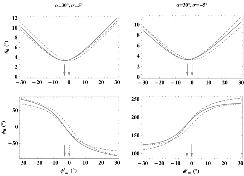
Figure 2: The magnetic colatitude $\theta_{0}$ and azimuth $\phi_{0}$ of the emission point as functions of rotation phase $\phi^{\prime}_{m}$ in the non-rotating (dotted curves) and the rotating (solid curves) cases. The dashed curves are those due to BCW (1991) model. Chosen $P=1$ s, and $r_{n}=r/r_{LC}=0.05.$ The dotted and solid arrows in the upper panels represent the location of $\theta_{0}$ minima while in the lower panels the location of inflection point of $\phi_{0}$ in non-rotating and rotating cases, respectively.

The magnetic colatitude $\theta_{0}$ and azimuth $\phi_{0}$ as functions of rotation phase $\phi^{\prime}_{m}$ are plotted in Figure 2 for both non-rotating (dotted curves) and rotating (solid curves) cases by using the parameters $\alpha=30^{\circ}$, $P=1$ s, $r_{n}=r/r_{LC}=0.05$ and $\sigma=\pm 5^{\circ}$ In the rotating case both the minimum of $\theta_{0}$ and inflection point of $\phi_{0}$ shift to the earlier rotation phase compared to those in non-rotating case. The absolute phase shifts of both $\theta_{0}$ minimum and the inflection point of $\phi_{0}$ from the fiducial phase $(\phi^{\prime}_{m}=0)$ are found to be $2.9^{\circ},$ which is about $\sim r_{n},$ as predicted by BCW (1991). For comparison we have superposed the curves (dashed line) due to BCW (1991) model, and find that their approximated analytical solutions are valid only over a smaller rotation phase around $2.9^{\circ}.$

Even though the observer receives maximum radiation from the emission point $(\theta_{0},\,\phi_{0})$ at which $\hat{v}$ and $\hat{n}$ are exactly aligned, observer receives a considerable radiation from the neighboring emission points too due to the finite width of emission beam. It is about $\sim 2/\gamma,$ and the boundary of the emission region centered on $\hat{n}$ is specified by the condition $\hat{n}\cdot\hat{v}=\cos(1/\gamma).$ For the computational purpose we discretized the beaming region into ‘beaming region points’ (BRP), and the coordinates $\theta$ and $\phi$ of each point is specified by $\theta_{e}$ and $\phi_{e},$ respectively. Since the coordinates $\theta$ and $\phi$ are orthogonal, their ranges $\theta_{e,min}\leq\theta\leq\theta_{e,max}$ and $\phi_{e,min}\leq\phi\leq\phi_{e,max}$ can be used to specify the beaming region boundary, where the subscripts (e,min) and (e,max) denote the lower and upper boundaries of the emission region. By considering $\theta_{0}-1/\gamma$ and $\theta_{0}+1/\gamma$ as initial guess values for $\theta_{e,min}$ and $\theta_{e,max}$ at $\phi=\phi_{0},$ we solve $\hat{n}\cdot\hat{v}=\cos(1/\gamma)$ numerically and find the roots $\theta_{e,min}$ and $\theta_{e,max}.$ Next for any $\theta=\theta_{e}$ within the range between $\theta_{e,min}$ and $\theta_{e,max}$, we consider $\phi_{0}-1/\gamma$ and $\phi_{0}+1/\gamma$ as the initial guess values for $\phi_{e,min}$ and $\phi_{e,max}$, and solve again $\hat{n}\cdot\hat{v}=\cos(1/\gamma)$ numerically to find the roots $\phi_{e,min}$ and $\phi_{e,max}.$ Note that beaming regions on leading side become broader compared to those on corresponding trailing ones, but, they are symmetric in the non-rotating case (Gangadhara, 2010). This is because the source trajectories on leading side get squeezed whereas on trailing side they get stretched (e.g., Thomas & Gangadhara, 2007).

Note that Equation (4) is the integration of the electric field of radiation emitted by the relativistic source along its trajectory. Observer receives the beamed radiation only for a small segment of source trajectory, say between the points $P_{i}$ and $P_{f}$ along a rotating field line (see Figure 1). As the source moves from $P_{i}$ to $P_{f}$ along the rotating field line, time changes from $t_{i}$ to $t_{f}$, colatitude $\theta$ changes from $\theta_{i}$ to $\theta_{f}$, and the rotation phase $\phi^{\prime}$ of magnetic axis changes from $\phi^{\prime}_{i}$ to $\phi^{\prime}_{f}$. From the relation $ds=|\textbf{b}|d\theta=\kappa c~{}dt$, we deduce the expression for time $t:$

$$t=\int\frac{|\textbf{b}|}{\kappa c}d\theta+K~{},$$ (5)

where $K$ is the integration constant. Using the condition $t=\phi^{\prime}_{m}/\Omega$ for all $\theta=\theta_{e}$ within the beaming region, it follows from Equation (5) that $K=(\phi^{\prime}_{m}/\Omega)-\left({\int{|\textbf{b}|/(\kappa c)}d\theta}\right)_{\rm\theta=\theta_{e}}$. Therefore we have

$$t=\frac{\phi^{\prime}_{m}}{\Omega}+\int\frac{|\textbf{b}|}{\kappa c}d\theta-\left({\int\frac{|\textbf{b}|}{\kappa c}d\theta}\right)_{\rm\theta=\theta_{e}}$$ (6)

and the corresponding $\phi^{\prime}=\Omega t$ for the source motion along any given field line within the beaming region. Hence the argument of the integrand in Equation (4) becomes function of $\theta$ only:

$$\textbf{E}(\textbf{r},\omega)=\frac{1}{\sqrt{2\pi}}\frac{qe^{i\omega R_{0}/c}}{R_{0}~{}c}\int^{+\infty}_{-\infty}\frac{|\textbf{b}|}{\kappa c}\frac{\hat{n}\times[(\hat{n}-\mbox{\boldmath$\beta$})\times\mbox{\boldmath$\dot{\beta}$}]}{\xi^{2}}e^{i\omega\left\{t-\hat{n}\cdot\textbf{r}/c\right\}}d\theta~{},$$ (7)

where time $t$ has to be replaced by the expression given in Equation (6).

Let

$$\textbf{A}=\{A_{i}\}=\frac{|\textbf{b}|}{\kappa c}\frac{\hat{n}\times[(\hat{n}-\mbox{\boldmath$\beta$})\times\mbox{\boldmath$\dot{\beta}$}]}{\xi^{2}}~{},$$ (8)

where $A_{i}$ with $i=x,~{}y$ and $z$, are the components of A in the $X,$ $Y$ and $Z$ directions, respectively (see Fig. 1). We series expand the components of A in powers of $\theta$ about $\theta_{e}$, and obtain

$$A_{i}(\theta)=a_{i0}+a_{i1}(\theta-\theta_{e})+a_{i2}(\theta-\theta_{e})^{2}+O[(\theta-\theta_{e})^{3}]~{},$$ (9)

where $a_{ij}$ with $i=x,~{}y$ and $z$, and $j=0,~{}1$ and $2$ are the series expansion coefficients. They are given by

$$a_{i0}=A_{i}(\theta_{e})~{},\quad a_{i1}=A^{\prime}_{i}(\theta_{e})~{},\quad a_{i2}=\frac{1}{2}A^{\prime\prime}_{i}(\theta_{e})~{},$$ (10)

where $A^{\prime}_{i}$ and $A^{\prime\prime}_{i}$ are the respective first and second derivatives of $A_{i}$ with respect to $\theta$ evaluated at $\theta_{e}$. Since the expressions of $a_{i0},$ $a_{i1},$ and $a_{i2}$ are too big, we have not reproduced them here. However one can always reproduce them by differentiating $\bf A.$

We set the argument of exponential in Equation (7), $\omega\left\{t-\hat{n}\cdot\textbf{r}/c\right\}=C,$ and series expand in powers of $\theta$ about $\theta_{e}$, and obtain

$$C(\theta)=c_{0}+c_{1}(\theta-\theta_{e})+c_{2}(\theta-\theta_{e})^{2}+c_{3}(\theta-\theta_{e})^{3}+O[(\theta-\theta_{e})^{4}]~{},$$ (11)

where $c_{k}$ with $k=0,~{}1,~{}2$ and $3$ are the series expansion coefficients. They are given by

$$c_{0}=C(\theta_{e})~{},\quad c_{1}=C^{\prime}(\theta_{e})~{},\quad c_{2}=\frac{1}{2}C^{\prime\prime}(\theta_{e})~{},\quad c_{3}=\frac{1}{6}C^{\prime\prime\prime}(\theta_{e})~{},$$ (12)

where $C^{\prime}$, $C^{\prime\prime}$, and $C^{\prime\prime\prime}$ are the respective first, second, and third derivatives of $C$ with respect to $\theta$ evaluated at $\theta_{e}$. Since the expressions of $c_{0},$ $c_{1},$ $c_{2}$ and $c_{3}$ are too big, we have not reproduced them here.

By substituting Equations (9) and (11) into Equation (7), we obtain the components of $\textbf{E}(\omega):$

$$E_{i}(\omega)=E_{0}\int^{+\infty}_{-\infty}(a_{i0}+a_{i1}\vartheta+a_{i2}\vartheta^{2})e^{i(c_{1}\vartheta+c_{2}\vartheta^{2}+c_{3}\vartheta^{3})}d\vartheta~{},$$ (13)

where $i=x,~{}y$ and $z.$ Here $\vartheta=\theta-\theta_{e}$ and $E_{0}=qe^{i[(\omega R_{0}/c)+c_{0}]}/(\sqrt{2\pi}R_{0}c).$

Next, by substituting the integral solutions $S_{0}$, $S_{1}$ and $S_{2}$ given in Appendix–A, we obtain

$$E_{i}(\omega)=E_{0}(a_{i0}S_{0}+a_{i1}S_{1}+a_{i2}S_{2})~{}.$$ (14)

The Stokes parameters: $I,$ $Q,$ $U$ and $V$ have been used as tools to specify the polarization state of the radiation field. The net radiation that the observer tends to receive at any rotation phase $\phi^{\prime}_{m}$ will be incoherent addition of radiation from bunches from all those emission points which lie within the beaming region. Following the definitions given by Gangadhara (2010), we estimate the resultant Stokes parameters $I_{s},$ $Q_{s},$ $U_{s}$ and $V_{s}.$

3 SIMULATION OF PULSE PROFILES

3.1 Emission From Beaming Region

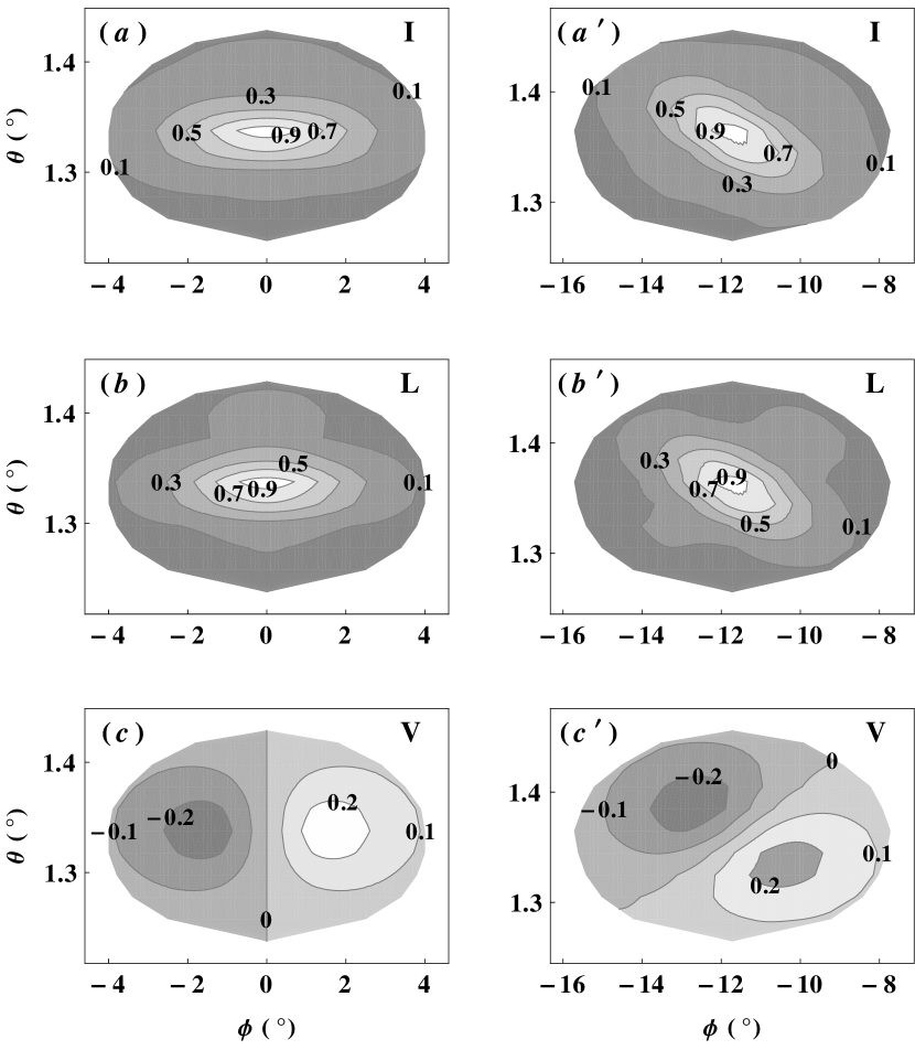
Figure 3: The simulation showing the emission from a beaming region due to an uniform distribution of sources in the non-rotating (left column panels) and the rotating (right column panels) cases at $\phi^{\prime}_{m}=0^{\circ}$. Chosen $\alpha=45^{\circ}$, $\sigma=2^{\circ}$, $r_{n}=0.01$, $P=1$ s, $\gamma=400$, and $\nu=600$ MHz.

By assuming uniform source distribution and using the viewing parameters: $\alpha=45^{\circ},$ $\sigma=2^{\circ},$ pulsar rotation period $P=1$ s, phase $\phi^{\prime}_{m}=0^{\circ}$, normalized emission height $r_{n}=0.01,$ particle’s Lorentz factor $\gamma=400$ and observation frequency $\nu=600$ MHz, we computed the Stokes parameters for the radiation field. The contour plots of $I,$ $L$ and $V$ in $(\theta,~{}\phi)$–plane are given in Figure 3. For comparison we present both the cases: non-rotating - panels (a), (b), and (c), and rotating - panels ($\textit{a}^{\prime}$), ($\textit{b}^{\prime}$), and ($\textit{c}^{\prime}$). The parameters $I,$ $L$ and $V$ are normalized with the corresponding maximum value of $I$ within the beaming region. We find the ratio of peak intensity in the rotating case to that in non-rotating is about 2. In all panels, the contour levels are marked on the respective contours. Also the contours are gray colored in such a way that darker the region lower the corresponding parameter value.

In the non-rotating case, the trajectory of the sources are same as their associated dipolar field lines. Hence the contours of $I$, and $L$ are symmetric, while those of $V$ are antisymmetric with respect to $(\theta,~{}\phi_{0})$ plane. In the rotating case, the contours of $I$, $L$, and $V$ gets rotated in ($\theta,~{}\phi$)–plane due to non-uniform aberration within BRP.

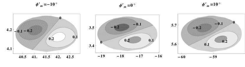
Figure 4: The simulation showing the circular polarization $V$ from the beaming region in the rotating case at three discrete rotation phases. Chosen $\alpha=30^{\circ}$, $\sigma=5^{\circ}$, $r_{n}=0.05$, $P=1$ s, $\gamma=400$ and $\nu=600$ MHz.

Using the parameters $\alpha=30^{\circ}$, $\sigma=5^{\circ}$, $r_{n}=0.05$, $P=1$ s, $\gamma=400$ and $\nu=600$ MHz at discrete rotation phases of the magnetic axis $\phi^{\prime}_{m}=-10^{\circ},$ $0^{\circ},$ and $10^{\circ}$, we simulated the emissions from the beaming region and presented the contours of $V$ in Figure 4. In each panel $V$ is normalized with the corresponding peak intensity $I_{peak}$ within the beaming region. The rotation of circular contour pattern is more towards the inner rotation phases $(\phi^{\prime}_{m}=0^{\circ})$ compared to that on outer rotation phases $(\phi^{\prime}_{m}=\pm 10^{\circ})$. This is because, the perpendicular distance from the pulsar spin axis to the beaming region decreases towards the outer rotation phases, and hence the smaller rotation effects. Further, circular contour pattern on the trailing side $(\phi^{\prime}_{m}=10^{\circ})$ gets more rotated compared to that on the leading side $(\phi^{\prime}_{m}=-10^{\circ})$. This is due to larger asymmetry in the intrinsic curvature of the field lines between the smaller and larger $\theta$ parts within the beaming region on the trailing side compared to that on the leading side.

To describe the behaviors of circular polarization and the swing of polarization position angle (PPA), we define the symbols: “+/-” for transition of $V_{s}$ from left-handed (LH) to right-handed (RH) and “-/+” for transition from RH to LH. Call the counterclockwise swing of PPA $(d\psi_{s}/d\phi^{\prime}_{m}>0)$ as “ccw” and the clockwise swing ($d\psi_{s}/d\phi^{\prime}_{m}<0)$ as “cw”.

3.2 Emission With Uniform Source Distribution

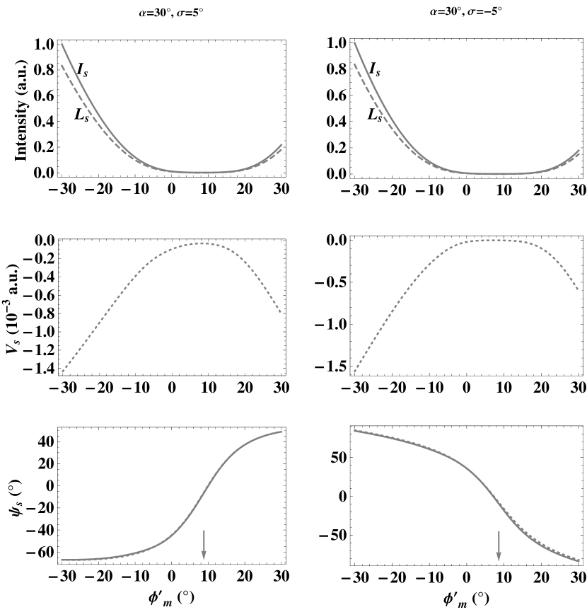
Figure 5: Simulated pulse profiles: chosen $P=1$ s, $\gamma=400$, $\nu=600$ MHz and $r_{n}=0.05$. In the $\psi_{s}$ panels: solid curves are due to our simulations and the dotted curves are due to BCW (1991) model. The arrows in the $\psi_{s}$ panels mark the polarization angle inflection point.

Assuming uniform source distribution and using the viewing parameters: $\alpha=30^{\circ},$ $\sigma=\pm 5^{\circ},$ $P=1$ s, $r_{n}=0.05,$ $\gamma=400$ and $\nu=600$ MHz, we computed the Stokes parameters for the curvature radiation. The profiles of $I_{s},$ $L_{s},$ $V_{s}$ and $\psi_{s}$ are plotted in Figure 5. The parameters in each panel are normalized with the corresponding maximum value of $I_{s}.$ In both the cases of $\sigma,$ $I_{s}$ becomes more stronger on leading side $(\phi^{\prime}_{m}<0^{\circ})$ of the fiducial phase $(\phi^{\prime}_{m}=0^{\circ})$ than on the trailing side. This is because, due to the rotation induced curvature, the source trajectories on leading side become more curved than on the trailing side. The dip in the intensity near $\phi^{\prime}_{m}=0^{\circ}$ is due larger radius of curvature $\rho$ compared to the other regions. The behavior of $L_{s}$ is similar to $I_{s}$ except it’s smaller values due to incoherent addition of radiation from bunches. We observe that a small quantity of circular polarization survives due to the rotation induced asymmetry. The polarization position angle is increasing (ccw) in the case of $\sigma=5^{\circ}$, whereas it is decreasing (cw) in the case of $\sigma=-5^{\circ}.$ The PPA inflection point, the phase at which $|d\psi_{s}/d\phi^{\prime}_{m}|$ is maximum (indicated by an arrow), is found to be shifted to $\phi^{\prime}_{m}=8.8^{\circ}$ for $\sigma=5^{\circ}$ and to $\phi^{\prime}_{m}=8.6^{\circ}$ for $\sigma=-5^{\circ}.$ These shifts are about $3~{}r_{n}.$

For comparison we have superposed BCW (1991) PPA curves (dotted curves) on our simulated PPA curves. Our simulated PPA profile shapes and the shift of PPA inflection point are found to be in good agreement with BCW (1991) model near the central parts $(\phi^{\prime}_{m}\sim 0)$ but slightly deviated at larger rotation phases due to the approximations made in the BCW (1991) model. Also, note that at any rotation phase $\phi^{\prime}_{m}$, BCW (1991) model considers only the emission from the central point of the beaming region, whereas we consider the emissions from the whole of the beaming region.

3.3 Emission With Modulation

In general pulsar average radio profiles consist of many components, which could be due to emission from plasma columns that are associated with sparks on polar cap. When sight line cuts through such emissions, it encounters intensity pattern, which may be treated as approximately Gaussians (e.g., Kramer et al., 1994). We consider time independent modulation (Gangadhara, 2010) so that any fluctuation in the intensity strength of individual pulses will be smoothed out and hence our simulated profiles are expected to resemble the pulsar average profiles. Consider a time independent Gaussian modulation in both the polar and azimuthal directions:

$$f(\theta,\phi)=\sum f_{0}\,\exp\left[-(\theta-\theta_{p})^{2}/\sigma_{\theta}^{2}\right]~{}\exp\left[-(\phi-\phi_{p})^{2}/\sigma_{\phi}^{2}\right]~{},$$ (15)

where $(\theta_{p},\phi_{p})$ define the peak location of the Gaussian and $f_{0}$ is the amplitude. The parameters $\sigma_{\theta}=\rm{w}_{\theta}/(2\sqrt{ln2})$ and $\sigma_{\phi}=\rm{w}_{\phi}/(2\sqrt{ln2})$, where $\rm{w}_{\theta}$ and $\rm{w}_{\phi}$ are the corresponding full width at half-maximum (FWHM) of the Gaussian in the two directions. The resultant Stokes parameters $I_{s},~{}Q_{s},~{}U_{s}~{}\rm{and}~{}V_{s}$ after taking into account of modulation are given in Gangadhara (2010).

3.3.1 Simulation of Core Emission

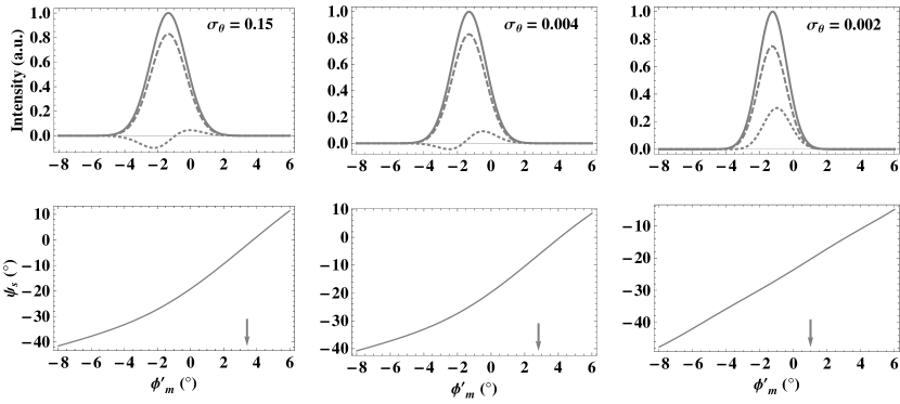
Figure 6: Simulated pulse profiles: Chosen $\alpha=10^{\circ},$ $\sigma=2^{\circ},$ $P=1$ s, $r_{n}=0.02,$ $\gamma=400$, $\nu=600$ MHz, $f_{0}=1,$ $\theta_{p}=1^{\circ},$ $\phi_{p}=0^{\circ}$ and $\sigma_{\phi}=0.15$. In each panel $I_{s}$ (solid curves), $L_{s}$ (dashed curves) and $V_{s}$ (dotted curves) are normalized with the respective peak intensity. The arrows in the $\psi_{s}$ panels mark the polarization angle inflection point.

To explore the effect of rotation on the central core component of pulsar radio profiles, we consider a Gaussian modulation having peak at ($\theta_{p},~{}\phi_{p})=(1^{\circ},~{}0^{\circ})$. We have chosen the peak of modulation slightly away from the magnetic axis to have modulation in both the $\theta$ and $\phi$ directions. For simulation, we used the viewing parameters: $\alpha=10^{\circ},$ $\sigma=2^{\circ},$ $P=1$ s, $r_{n}=0.02,$ $\gamma=400$ and $\nu=600$ MHz. Since the minimum of the coordinate $\theta$ is $\sim 2/3~{}\sigma=1.33^{\circ}$ in this case, sight line passes through the emission region where modulation strength is slightly below its amplitude. To see the combined effect of rotation and modulation, we considered $\sigma_{\phi}=0.15$ and three cases for $\sigma_{\theta}=0.15,$ 0.004 and 0.002, and the simulated polarization profiles are given in Figure 6. In all the three cases of $\sigma_{\theta}$, intensity profiles are shifted to earlier phase with respect to the fiducial phase $\phi^{\prime}_{m}=0^{\circ}$ while the polarization position angle profile shifts to the later phase due to effect of rotation. Note that in the absence of rotation, the minimum of $\theta_{0}$ and the antisymmetric point of $\phi_{0}$ (i.e., phase at which $\phi_{0}=0$) occur at $\phi^{\prime}_{m}=0^{\circ}$ and hence the intensity will peak at $\phi^{\prime}_{m}=0^{\circ}.$ But in the rotating case intensity peaks shift to earlier phases by about $1.36^{\circ},$ $1.31^{\circ}$ and $1.24^{\circ}$ in the three cases of $\sigma_{\theta}=0.15,$ 0.004 and 0.002, respectively. The phase shift of $I_{s}$ peak is found to decrease with decreasing $\sigma_{\theta}.$ The reasons are, due to aberration, the minimum of $\theta_{0}$ and the antisymmetric point of $\phi_{0}$ and hence the peak of modulation (phase at which observer encounters maximum modulation strength) shift to earlier phase. But the emission due to uniform source distribution becomes more stronger on the leading side of the modulation peak compared to that on the trailing side. Therefore, the peak of modulated total intensity will be further advanced in phase with respect to the peak of modulation. However this extra phase shift of modulated intensity peaks with respect to modulation peaks favor the formation of a more symmetric component: larger unmodulated emission on smaller radius of curvature side will be less enhanced by weaker modulation whereas smaller unmodulated emission on larger radius of curvature side will be more enhanced by stronger modulation. Note that if the modulation is more steeper then the intensity profile closely follows the modulation. Hence the pulse width and the phase shift of peak of the total intensity will decrease as we go from $\sigma_{\theta}=0.15$ to $\sigma_{\theta}=0.002.$

In the case of $\sigma_{\theta}=0.15$, the circular polarization is antisymmetric and the transition is from RH (negative) to LH (positive). The leading negative circular is found to be more stronger compared to that on the trailing positive circular, whereas they are equal in the non-rotating case (Gangadhara, 2010). The asymmetry in the strengths of negative and positive circulars can be explained as follows: due to rotation , the pattern of circular polarization (see Figure 3) gets rotated in the $(\theta,~{}\phi)$–plane and hence an asymmetry is introduced in both $\theta$ and $\phi$ directions. Since we used $\theta_{p}=1^{\circ}$ and the minimum of $\theta$ that the observer encounters is $\sim 1.3^{\circ},$ the modulation in the $\theta$ direction always enhance the emission over smaller values of $\theta$ (see Figure 3) compared to that over larger values of $\theta$ within the beaming region. Further, since we used $\phi_{p}=0^{\circ}$, modulation in $\phi$ direction selectively enhance the emissions over smaller values of $|\phi|$ compared to those over larger values of $|\phi|$ within the beaming region. Since $\sigma_{\phi}=\sigma_{\theta}$ and beaming regions are more extended in $\phi$ compared to those in $\theta$, the modulation gradient in $\phi$ dominates over that in $\theta$. Further, the magnitude of rotation of circular polarization pattern within the beaming region is more for the inner rotation phases (phases closer to $\phi^{\prime}_{m}=0^{\circ}$) as compared to that on outer phases (see Figure 4). Hence modulation can selectively enhance the leading negative circular over the trailing positive circular. Also, because of above said reasons, the phase location of the sign reversal of circular is found to be lagging the phase location of the peak of total intensity by a small amount.

In the case of $\sigma_{\theta}=0.004,$ the trailing positive circular becomes more stronger than the leading negative circular, which is opposite to $\sigma_{\theta}=0.15.$ Even though the effect of rotation on the pattern of circular polarization is same as in the case of $\sigma_{\theta}=0.15,$ the modulation becomes comparatively stronger in the $\theta$ direction as $\sigma_{\theta}\ll\sigma_{\phi}.$ Hence, on the leading side, the net two dimensional modulation selectively enhances emission over the lower left part of the beaming region, whereas on the trailing side, it selectively enhance the emission over the lower right part (see Figure 4). Hence the positive circular on the trailing side becomes more stronger compared to negative circular on the leading side. Due to above said reasons, the phase of sign reversal of circular is found to be leading the phase of total intensity peak by a small amount.

In the extreme case of $\sigma_{\theta}=0.002$, modulation becomes much more stronger in the $\theta$ direction. Therefore the modulation selectively enhances the emission over the lower part of the beaming region through out the pulse window. Hence the circular polarization becomes almost positive through out the pulse. Again due to asymmetry in the magnitude of rotation of the circular polarization pattern with respect to rotation phase $\phi^{\prime}_{m},$ the survived positive circular is found to be more stronger on the trailing side as compared to that on leading side.

In all the three cases, $L_{s}$ almost follows $I_{s}$ except for its magnitude. Further, when $V_{s}$ is weaker $L_{s}$ is found to be little stronger and vice versa. In all the three cases, PPA swing is ‘ccw’ and PPA inflection points (indicated by arrows) are found to be shifted to later phases by $3.42^{\circ},$ $2.82^{\circ}$ and $1.00^{\circ}$, respectively. The phase shift of the position angle inflection point is found to decrease with decreasing $\sigma_{\theta}$ due to the combined effect of rotation and modulation.

BCW (1991) have predicted that due to aberration both the $\theta$ minimum and the antisymmetric point of $\phi$ shift to earlier phase by $\sim r_{n},$ $(1.14^{\circ}~{}\rm{for}~{}r_{n}=0.02),$ with respect to the fiducial phase $\phi^{\prime}_{m}=0^{\circ}.$ They assumed that the centroid of the intensity profile coincides with the $\theta$ minimum and the antisymmetric point of $\phi$. Further, by using the particle acceleration vector, which reflects direction of the electric field vector in time domain, BCW (1991) have also predicted that the shift of PPA inflection point to later phase by $\sim 3~{}r_{n},$ $(3.44^{\circ}~{}\rm{for}~{}r_{n}=0.02).$ However, in our model, we estimate the radiation field in frequency domain. We consider the effect of rotation along with modulation and a detailed geometry of emission region which includes finite beaming regions from which the observer can receive the considerable radiation, which is not considered in the BCW (1991) model. Hence the phase shifts of total intensity and PPA inflection points can be significantly different from those predicted by BCW (1991).

Note that if one considers the retardation (radiation propagation time delay), the emissions from the beaming region at any rotation phase $\phi^{\prime}_{m}$ will be arrived at later time, i.e., by delay $\delta t=\hat{n}\cdot\textbf{r}/c$, and hence phase delayed by $\delta\phi^{\prime}_{ret}=\Omega\delta t$ (e.g., Gangadhara, 2005). However since we have assumed that emissions from the whole beaming region originate from a particular altitude $r$ for a given phase $\phi^{\prime}_{m}$, they will have roughly the same $\delta t\sim r/c$ (which at most differ by $\sim 10^{-8}s$ between center to boundary within the beaming region). Hence emissions will arrive at the same time $t_{r}=t_{e}+\delta t$, where $t_{e}~{}\rm{and}~{}t_{r}$ are the emission and reception times of the radiation, respectively. Further, since we consider a constant $r$ across the whole pulse, the net emission due to whole beaming region at any phase $\phi^{\prime}_{m}$ will be time delayed by the same $\delta t\sim r/c.$ Hence a constant phase delay of $\delta\phi^{\prime}_{ret}\sim\Omega r/c=r/r_{LC}=r_{n}$ across the whole pulse is introduced. After taking into account of retardation along with aberration, the phase shifts of intensity peak and PPA inflection point for example in the case $\sigma_{\theta}=0.15$ of Figure 6 will be $2.50^{\circ}~{}\rm{and}~{}2.28^{\circ}$, respectively. Since retardation just causes the shift of entire aberrated profile by $\delta\phi^{\prime}_{ret}$ to the earlier phase, we have not reproduced simulations by combining retardation along with aberration. However the shapes of the aberrated profile will be affected if one considers the varying altitude across the pulse.

Also note that if one considers the modulation which is broader than the one considered in the case of $\sigma_{\phi}=\sigma_{\theta}=0.15$ of Figure 6, then the aberration phase shift of the intensity peak becomes substantially different from $r_{n}.$ Further $V_{s}$ becomes almost symmetric type with negative circular through out the profile. This is because as modulation becomes broader pulse also becomes broader. Further in Figure 6, we kept $\sigma_{\phi}$ constant and varied $\sigma_{\theta}$ for the three cases. On the other hand if one considers the case in which $\sigma_{\theta}$ is kept constant and $\sigma_{\phi}$ is varying from more broader modulation to steeper one, then the behavior of total intensity and PPA profiles will be similar to Figure 6. But the evolution of $V_{s}$ will be from almost symmetric type to antisymmetric type due to above mentioned reasons. Also, if one considers the case in which both the $\sigma_{\phi}$ and $\sigma_{\theta}$ vary by the same amount from more broader modulation to steeper one, then the behavior of pulse profiles will be similar to the case wherein $\sigma_{\theta}$ is kept constant and $\sigma_{\phi}$ is varying from larger to smaller value. Further if one considers the negative $\sigma$ then the polarization profiles behave similar to the positive $\sigma$ except for the fact that the polarities of $V_{s}$ and swing of PPA profile will be opposite.

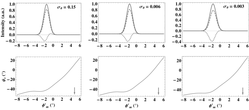
Figure 7: Simulated pulse profiles: Chosen $\sigma=1^{\circ}$ and the other parameters same as in Figure 6.

To see the combined effect of rotation and modulation in the case of sight line passing through the other side of the emission region which lies towards the magnetic axis, we considered the sight line with $\sigma=1^{\circ}.$ For simulations we kept the other parameters the same as those of $\sigma=2^{\circ}$ case of Figure 6. The simulated polarization profiles for $\sigma_{\phi}=0.15$ and the three cases $\sigma_{\theta}=0.15,$ 0.006 and 0.003 are given in Figure 7. The phase shifts of the total intensity peak in the cases $\sigma_{\theta}=0.15,$ 0.006 and 0.003 are found to be $1.44^{\circ},$ $1.46^{\circ}$ and $1.53^{\circ},$ respectively. The phase shift of the intensity peak tends to increase with decreasing $\sigma_{\theta}$, a behavior opposite to the case of $\sigma=2^{\circ}$ (see Figure 6). This is because, since we have chosen $\theta_{p}=1^{\circ}$, the emission point coordinate $\theta$ will be closer to $\theta_{p}$ at the outer rotation phases $|\phi^{\prime}_{m}|>0^{\circ}.$ But the minimum of the emission point coordinate $|\phi|$ will be closer to chosen $\phi_{p}=0^{\circ}$ for the inner earlier rotation phases. Therefore, the modulation mapped onto a broader pulse phase as $\sigma_{\theta}$ decreases. Hence, the phase shift of intensity peak increases as we go from $\sigma_{\theta}=0.15$ to 0.003.

In the case of $\sigma_{\theta}=0.15$ circular polarization is marginally antisymmetric and the transition is from negative to positive. The leading negative circular is found to be much more stronger than the trailing positive circular compared to $\sigma_{\theta}=0.15$ of Figure 6. Due to viewing geometry observer tends to receive radiation from the beaming region whose emission points in $\theta$ are always less than $\theta_{p}=1^{\circ}$ in this case. Hence the net modulation selectively enhances emission over the upper left part of the beaming region (see Figure 4) on the leading side, whereas it selectively enhances the emission over the upper right part of the beaming region on the trailing side. Hence from Figure 4 we see that the leading negative circular becomes much more stronger than the trailing positive circular. The phase lag of the location of sign reversal of circular with respect to intensity peak is found to be more compared to that in the case of $\sigma=2^{\circ}$ and $\sigma_{\theta}=0.15.$ In the case of $\sigma_{\theta}=0.006,$ the negative circular becomes even more stronger compared to positive circular, and in the extreme case of $\sigma_{\theta}=0.003$, circular becomes symmetric, i.e., only negative circular survives through out the pulse.

In all the three cases, the position angle swing is ‘ccw’ and the phase shifts of its inflection point for $\sigma_{\theta}=0.15,$ 0.006 and 0.003 are found to be $4.80^{\circ},$ $4.87^{\circ}$ and $4.97^{\circ},$ respectively. The phase shift of the position angle inflection point is found to increase with decreasing $\sigma_{\theta}$ unlike in the case of $\sigma=2^{\circ}$ where it decreases with decreasing $\sigma_{\theta}.$ The observed opposite trend in the phase shift of the PPA inflection point with respect to modulation parameter $\sigma_{\theta}$ is because of opposite trend in the selective enhancement of the emission over a part of the beaming region in the two cases of $\sigma$.

Note that so far we have considered the general cases of core modulation where the modulation peak is located slightly away from the magnetic axis and modulated in both $\theta$ and $\phi$ coordinates. The more plausible case for core modulation is a Gaussian whose peak is located at the magnetic axis, i.e., at $\theta_{p}=0^{\circ}$ and depends only in $\theta.$ The corresponding modulation function that follows from Equation (15) is $f(\theta)=f_{0}\,\exp(-\theta^{2}/\sigma_{\theta}^{2}).$ If one simulates the pulse profiles with this modulation, $V_{s}$ becomes symmetric type: positive circular (LH) for positive $\sigma$ and negative circular (RH) for negative $\sigma$ through out the pulse due to the selective enhancement. Note that in the non-rotating model (Gangadhara, 2010), the modulation in only $\theta$ direction will never give the considerable net circular irrespective of its gradient, as it always enhance both the positive and negative circulars by the same amount (see panel (c) in Figure 3).

3.3.2 Simulation of Conal Emission

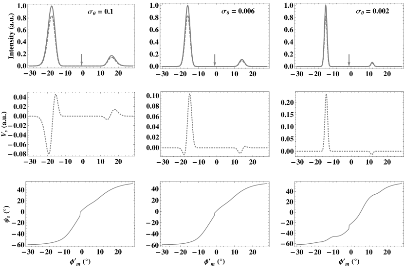
Figure 8: Simulated pulse profiles: The parameters chosen are same as in Figure 6 except $(\theta_{p},\,\phi_{p})=(2^{\circ},\,\pm 65^{\circ})$ and $\sigma_{\phi}=0.1.$

In this section we consider the combined effect of rotation and modulation on the concentric conal emissions. Consider two Gaussians whose peaks are situated at $(\theta_{p},~{}\phi_{p})=(2^{\circ},~{}\pm 65^{\circ})$ and rest of the parameters the same as in Figure 6. The modulation peak locations are chosen such that the sight line passes through the emission regions with modulation strengths below its amplitude and the region of maximum modulation encountered by the observer lies towards the meridional plane. The simulated polarization profiles are given in Figure 8 for the three cases of $\sigma_{\theta}=0.1,$ 0.006 and 0.002. In all the three cases leading side component becomes more stronger than the trailing side component. This is due to the combined effect of enhancement in the intrinsic unmodulated emission and the modulation strength on leading side over the trailing side. However the enhancement due to unmodulated emission is more prominent. In the IOF, due to aberration, the plasma bunch trajectories become more curved on leading side compared to those on trailing side, and hence more emission occurs on leading side. The marginal decrease in the strength of trailing side component as we go from the case $\sigma_{\theta}=0.1$ to $0.002$ is due to weaker modulation that the sight line encountered on trailing side. Further in all the cases of $\sigma_{\theta},$ the trailing side component becomes considerably narrower than the leading side component. This is because, even though the modulation has roughly the same steepness on both the leading and trailing sides, the radius of curvature becomes more steeper in phase on trailing side compared to that on the leading side. Hence it results in a broader component on leading side. The phase shifts of the mid point of intensity peaks (the cone centers indicated by arrows) to the earlier phase in the cases $\sigma_{\theta}=0.1,~{}0.006,~{}\rm{and}~{}0.002$ are found to be $0.74^{\circ}$, $0.94^{\circ}$ and $1.10^{\circ},$ respectively.

In the case of $\sigma_{\theta}=0.1,$ negative circular becomes more stronger compared to positive circular on leading side whereas it is vice versa on the trailing side. This is because, the magnitude of rotation of circular pattern is more for inner rotation phases while the net modulated emission is slightly smaller compared to outer phases and hence selective enhancement of outer side circulars within the intensity components. In the case of $\sigma_{\theta}=0.006,$ positive circular became more stronger compared to negative circular over the leading side component and vice versa over the trailing side component. In the case of $\sigma_{\theta}=0.1,$ the modulation is broader and hence sight line encounters both the parts of modulation which are lying towards and away from the meridional plane. As $\sigma_{\theta}$ decreases, observer tends to selectively encounter the parts of modulation which are closer to meridional plane. This selectively enhances the $V_{s}$ which lies towards $\phi_{m}=0^{\circ}.$ Hence the inner sides of $V_{s}$ become more stronger as compared to outer sides over both the leading and trailing sides of $I_{s}.$ In the extreme case of $\sigma_{\theta}=0.002$, $V_{s}$ becomes symmetric type, i.e., only positive on leading side and negative on the trailing side.

In all the cases of $\sigma_{\theta}$ linear polarization $L_{s}$ profile almost follows the total intensity $I_{s},$ and PPA swing is ‘ccw’. The distortions or kinks are due to combined effect of rotation and modulation on the emissions over the beaming regions. The phase shift of the PPA inflection point has become uncertain as the kinks are affecting the central part of the position angle curves. However if one considers a case where central core component lies between two conal components then the position angle inflection point can be found without difficulty.

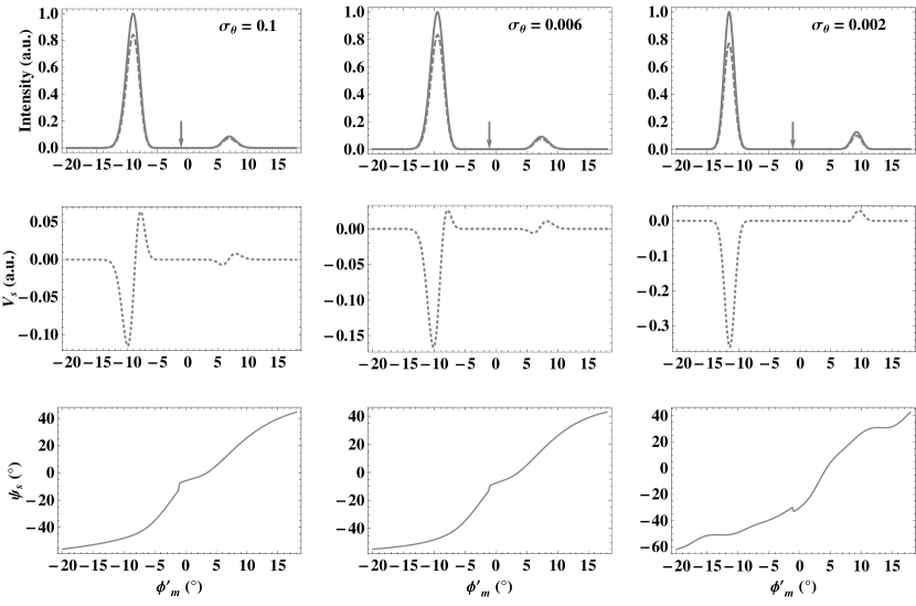
Figure 9: Simulated pulse profiles: The parameters chosen are same as in Figure 8 except $\phi_{p}=\pm 40^{\circ}.$

As a next case, we select the modulations with peaks at different azimuthal locations $(\phi_{p}=\pm 40^{\circ})$ on the same conal ring which is considered in Figure 8. In this case sight line passes through the emission regions with modulation strengths below its amplitude and the region of maximum modulation encountered by the observer lies away from the meridional plane. By keeping other viewing parameters same as in the case of Figure 8, we simulated the polarization profiles for the cases of $\sigma_{\theta}=0.1,$ 0.006 and 0.002 and given in Figure 9. The small increase in the strength of the trailing side component as we go from $\sigma_{\theta}=0.1$ to 0.002 is due to an increase in the modulation strength that the observer encounters on the trailing side. The phase shift of the cone centers to the earlier phase in the cases $\sigma_{\theta}=0.1,$ 0.006 and 0.002 are found to be $1.07^{\circ},$ $1.06^{\circ}$ and $1.08^{\circ}$, respectively. These shifts are found to be almost independent of $\sigma_{\theta}$ unlike in the previous cases where they considerably dependent on the $\sigma_{\theta}.$ In the case of $\sigma_{\theta}=0.1,$ $V_{s}$ is antisymmetric on both the leading and trailing sides with the outer circular is more stronger than the inner. This is similar to the cases $\sigma_{\theta}=0.1$ in Figure 8, where the modulation is broader. In the case of $\sigma_{\theta}=0.006$, $V_{s}$ is again antisymmetric on both leading and trailing sides but outer circular dominates over the inner. This is because, sight line encounters the major part of the modulation, which lies away from the meridional plane. Hence there is a selective enhancement of the outer circular relative to the inner. In the extreme case of $\sigma_{\theta}=0.002$, $V_{s}$ becomes symmetric on both the sides: negative on leading side and vice versa on the trailing. These are of opposite behaviors as compared to Figure 8. In all the three cases of $\sigma_{\theta}$, $L_{s}$ almost follows the $I_{s}$ with lower values similar to the previous cases, and the PPA swing is ‘ccw’ and shows the kinky behavior.

4 DISCUSSION

Pulsar rotation along with modulation and viewing geometry seems to be greatly influencing the pulsar radio profiles. Due to rotation the trajectories of sources on leading side becomes more curved compared to those on trailing side, and hence leading side unmodulated emission always dominate over the trailing one. If one considers an azimuthally symmetric cone modulations then the leading side intensity components become more stronger than the corresponding trailing ones due to the rotationally induced asymmetry in the curvature of plasma trajectories (e.g., Thomas & Gangadhara, 2007). In support of this there is a strong observational result by Lyne & Manchester (1988), and our simulations clearly confirm it. We also find that the leading side intensity components become wider than the corresponding trailing ones due to an asymmetry in the gradient of radius of curvature between leading and trailing sides. These findings have an observational evidence (Ahmadi & Gangadhara, 2002) and a similar behavior has been discussed by Dyks, Wright & Demorest (2010). Note that if we consider higher emission altitude in our simulations then the trailing side component gets substantially weaker or even vanishing. Hence it could serve as an explanation for the “partial cones” (Thomas, Gupta & Gangadhara, 2010).

The fact that the phase shift of the intensity components to earlier rotation phases and that of the PPA inflection point to later phase is a natural consequence of effect of rotation. The phase shifts of the centroid of pulse and that of the PPA inflection points have been predicted to be about $r_{n}$ and $3r_{n}$, respectively (BCW, 1991). But in their simplistic model considered only the emission from the points at which source velocity vector exactly aligns with the observer’s sight line. However there is a considerable emission from the other points of beaming region, which is influenced by rotation and modulation. As a result the shifts of intensity component and PPA inflection point will no longer remain as $r_{n}$ and $3r_{n},$ respectively. We have shown that, due to pulsar corotation, the pattern of emission within the beaming region gets rotated in $(\theta,\phi)$–plane, and hence an asymmetry is introduced in both the $\theta$ and $\phi$ directions. Due to these asymmetries within the beaming region, either the antisymmetric or symmetric type circular polarization become possible depending upon the viewing geometry and modulation. If the modulation is more steeper and has roughly the same gradient in both $\theta$ and $\phi$, then the antisymmetric circular polarization is observed. On the other hand the symmetric type circular polarization is more plausible when modulation is broader and has roughly the same gradient in both $\theta$ and $\phi,$ and also when modulation is more steeper in $\theta$ than in $\phi.$ But in literature, circular polarization has been modeled only in the non-rotating pulsar approximation. Hence only the antisymmetric circular polarization was thought to be a natural feature of curvature radiation, and the symmetric type circular polarization was speculated to be a consequence of propagation effect (e.g., Gil, Kijak & Zycki, 1993; Gangadhara, 2010).

Han et al. (1998) and You & Han (2006) have found that the sign reversal of circular polarization is not only associated with the central ‘core’ region but also found over conal components as well as at the intersection of conal components. From our simulations of conal components, it is possible to explain all types of circular polarization sense reversals and its association with either increasing or decreasing PPA of Table 3 in You & Han (2006). For example, consider the Figures 8 and 9 in the case of $\sigma_{\theta}=0.1.$ On the leading side, we get a case where the circular polarization changes sign from negative to positive with an increasing PPA. Again by considering the $\sigma_{\theta}=0.002$ cases of Figures 8 and 9, on leading side we can get a case where circular polarization changes sign from positive to negative with increasing PPA.

We do confirm the Radhakrishnan & Rankin’s (1990) correlation that the sense reversal of circular polarization from negative to positive is correlated with ‘ccw’ PPA swing (or increasing PPA) and vice versa, and we argue this as a geometric property of curvature radiation. In pulsars with ‘symmetric’ type of circular polarization, Han et al. (1998) have not found any correlation between the sense of circular polarization and the PPA swing. Our simulations also indicate that the negative circular polarization can be associated with either ‘ccw’ or ‘cw’ PPA swing depending upon the viewing geometry and modulation locations. Similarly the positive circular too can be associated with ‘ccw’ or ‘cw’ PPA swing. However, Han et al. (1998) and You & Han (2006) have found that many conal–double pulsars show a single handed circular polarization over both the components. The negative circular correlated with the ‘ccw’ PPA swing and the positive circular with the ‘cw’ PPA swing.

Our simulations of conal components show that if the sight line is missing the modulation peaks and the steepness of modulation in the polar ($\theta$) direction is much larger as compared to that in the azimuthal ($\phi$) direction, then the circular polarization becomes single handed on both the leading and trailing sides but have opposite signs (see for example case $\sigma_{\theta}=0.002$ of Figures 8 and 9). Note that we considered situations where the leading and trailing side modulations symmetrically lie on a cone centered on the magnetic axis. On the other hand if one considers a situation where the modulations are asymmetrically located on a cone, then the correlation between the sense of circular polarization and the PPA swing in the case of conal-double pulsars can be explained. For example, by choosing the locations of modulations in the case of $\sigma_{\theta}=0.002$ of Figure 9 at $\phi_{p}=40^{\circ}$ and $-65^{\circ}$, one can get negative circulars over both the leading and trailing components (see the cases $\sigma_{\theta}=0.002$ of Figures 8 and 9), and hence an association of negative circular with the increasing PPA can be established.

The ‘kinky’ type distortion in PPA profile has been found in some normal pulsars and more commonly in millisecond pulsars. Mitra et al. (2000) have attributed this effect to multi polar magnetic field while Mitra & Seiradakis (2004) have speculated that the aberration/retardation resulting from the height-dependent emission can cause the distorted PPA traverses. Ramachandran & Kramer (2003) following Hibschman & Arons (2001) have proposed that the discrete jumps in the PPA profiles are due to magnetospheric return currents. However, from our simulations it is clear that even with a constant emission altitude across the whole pulse profile the ‘kinky’ behaviors can be produced in PPA traverses. Due to an incoherent addition of radiation field emitted from a beaming region, which is affected by rotation and modulation, the distortions in the PPA traverses are introduced. The PPA traverse under both the core as well as conal components are found to get distorted. But there are observational claims that central core region is more likely to show RVM distortions than the conal regions (e.g., Rankin, 1983, 1990; Radhakrishnan & Rankin, 1990).

In this work we considered a constant emission altitude $r$ across the whole pulse to make comparison with the earlier results. However varying emission altitude across the pulse can be incorporated. We considered only the rotation and time independent modulation effects in our simulations, as we are interested in the polarization properties of curvature radiation which is of intrinsic origin. We plan to consider the propagation effects, polar cap currents, magnetic field sweep back and higher multi polar components of magnetic field on pulsar radio emission in our future works.

5 CONCLUSION

By developing a relativistic model for pulsar radio emission we have attempted to explain the complete polarization state of the curvature radiation. Our model takes into account of a very detailed geometry of emission region, rotation and modulation as detailed in section 3.3, which have not been much incorporated in the earlier models. Based on our pulse profile simulations, we conclude the following:

1. The phase shift of intensity components to earlier phase and the PPA inflection point to later phase, are strongly influenced by the combined effect of rotation and the modulation.

2. The components on the leading side become stronger and broader than those on the trailing side because of rotation.

3. In an unmodulated emission a small quantity of circular polarization survives due to rotationally induced asymmetry, but from the point of view of observations it is insignificant.

4. For the very first time we are able to show that the ‘symmetric’ type circular polarization can be obtained within the frame work of curvature radiation. This result is very important from the point of view of emission mechanism.

5. Both the types of circular polarization: antisymmetric $(+/-$ or $-/+)$ and symmetric $(+$ or $-),$ can result any where within the pulse window due to the combined effect of rotation, viewing geometry and modulation. This might be responsible for the diverse nature of circular polarization.

6. We argue that pulsar rotation combined with modulation can introduce ‘kinky’ patterns into the PPA traverses.

APPENDIX–A:

Consider the integral

$$S_{0}=\int\limits_{-\infty}^{+\infty}{e}^{i(c_{1}\,\vartheta+c_{2}\,\vartheta^{2}+c_{3}\,\vartheta^{3}})d\vartheta~{}.$$ (A-1)

By changing the variable of integration $\vartheta=(x/l)+m,$ and defining the constants $l=\sqrt[3]{3c_{3}}$ and $m=-c_{2}/(3c_{3}),$ we obtain

$$\int\limits_{-\infty}^{+\infty}{e}^{i(c_{1}\,\vartheta+c_{2}\,\vartheta^{2}+c_{3}\,\vartheta^{3})}d\vartheta=U\int\limits_{-\infty}^{+\infty}e^{i\left(zx+\frac{x^{3}}{3}\right)}dx~{},$$ (A-2)

where $z=\frac{1}{\sqrt[3]{3c_{3}}}\left(c_{1}-\frac{c_{2}^{2}}{3c_{3}}\right)$ and $U=\frac{1}{\sqrt[3]{3c_{3}}}e^{i\frac{c_{2}}{3c_{3}}\left(\frac{2c_{2}^{2}}{9c_{3}}-c_{1}\right)}.$

For ${\rm Im}(z)=0,$ we know

$$j_{0}=\int\limits_{-\infty}^{\infty}{\rm e}^{i\left(zx+\frac{x^{3}}{3}\right)}dx=2\pi Ai(z),$$ (A-3)

where Ai$(z)$ is an entire Airy function of z with no branch cut discontinuities, and

$$j_{1}=\int\limits_{-\infty}^{\infty}x{e}^{i\left(zx+\frac{x^{3}}{3}\right)}dx=-i2\pi Ai^{\prime}(z)~{},$$ (A-4)

where $Ai^{\prime}(z)$ is the derivative of the Airy function $Ai(z).$ Therefore, we have

$$S_{0}=U~{}j_{0}~{}.$$ (A-5)

By differentiating equation (A-2) with respect to $c_{1},$ we obtain

$$S_{1}=\int\limits_{-\infty}^{+\infty}\vartheta{e}^{i(c_{1}\vartheta+c_{2}\vartheta^{2}+c_{\rm 3}\vartheta^{3})}d\vartheta = \frac{U}{\sqrt[3]{3c_{3}}}\int\limits_{-\infty}^{+\infty}\left(x-\frac{c_{2}}{\sqrt[3]{3c_{3}^{2}}}\right)e^{i\left(z\,x+\frac{x^{3}}{3}\right)}dx~{}$$ (A-6)

$$= \frac{U}{\sqrt[3]{3c_{3}}}\left(j_{1}-\frac{c_{2}}{\sqrt[3]{9c_{3}^{2}}}j_{0}\right)~{}.$$

Differentiation of equation (A-2) with respect to $c_{2}$ gives

$$S_{2}=\int\limits_{-\infty}^{+\infty}\vartheta^{2}{e}^{i(c_{1}\vartheta+c_{2}\vartheta^{2}+c_{3}\,\vartheta^{3})}d\vartheta = \frac{U}{3c_{3}}\int\limits_{-\infty}^{+\infty}\left(\frac{2c_{2}^{2}}{3c_{3}}-c_{1}-\frac{2c_{2}}{\sqrt[3]{3c_{3}}}x\right)e^{i\left(zx+\frac{x^{3}}{3}\right)}dx~{}$$ (A-7)

$$= \frac{U}{3c_{3}}\left[\left(\frac{2c_{2}^{2}}{3c_{3}}-c_{1}\right)j_{0}-\frac{2c_{2}}{\sqrt[3]{3c_{3}}}j_{1}\right]~{}.$$

References

- Ahmadi & Gangadhara (2002) Ahmadi, P., & Gangadhara, R. T. 2002, ApJ, 566, 365
- BCW (1991) Blaskiewicz, M., Cordes, J. M., & Wasserman, I. 1991, ApJ, 370, 643
- Cheng & Ruderman (1979) Cheng, A. F., & Ruderman, M. A. 1979, ApJ, 229, 348
- Cheng & Ruderman (1980) Cheng, A. F., & Ruderman, M. A. 1980, ApJ, 235, 576
- Dyks (2008) Dyks, J. 2008, MNRAS, 391, 859
- Dyks, Rudak & Harding (2004) Dyks, J., Rudak, B., & Harding, A. K. 2004, ApJ, 607, 939
- Dyks, Wright & Demorest (2010) Dyks, J., Wright, G. A. E., & Demorest, P. 2010, MNRAS, 405, 509
- Gangadhara (1997) Gangadhara, R. T. 1997, A&A, 327, 155
- Gangadhara & Gupta (2001) Gangadhara, R. T., & Gupta, Y. 2001, ApJ, 555, 31
- Gangadhara (2004) Gangadhara, R. T. 2004, ApJ, 609, 335
- Gangadhara (2005) Gangadhara, R. T. 2005, ApJ, 628, 923
- Gangadhara (2010) Gangadhara, R. T. 2010, ApJ, 710, 29
- Gil & Snakowski (1990a) Gil, J. A., & Snakowski, J. K. 1990a, A&A, 234, 237
- Gil & Snakowski (1990b) Gil, J. A., & Snakowski, J. K. 1990b, A&A, 234, 269
- Gil, Kijak & Zycki (1993) Gil, J. A., Kijak, J. & Zycki, P. 1993, A&A, 272, 207
- Gupta & Gangadhara (2003) Gupta, Y., & Gangadhara, R. T. 2003, ApJ, 584, 418
- Han et al. (1998) Han, J. L., Manchester, R. N., Xu, R. X., & Qiao, G. J., 1998, MNRAS, 300, 373
- Hibschman & Arons (2001) Hibschman, J. A., & Arons, J. 2001, ApJ, 546, 382
- Kazbegi, Machabeli & Melikidze (1991) Kazbegi, A. Z., Machabeli, G. Z., & Melikidze, G. J. 1991, MNRAS, 253, 377
- Komesaroff (1970) Komesaroff, M. M. 1970, Nature, 225, 612
- Kramer et al. (1994) Kramer, M., Wielebinski, R., Jessner, A. , Gil, J. A. & Seiradakis, J. H. 1994, A&AS, 107, 515
- Krzeszowski et al. (2009) Krzeszowski, K., Mitra, D., Gupta, Y., Kijak, J., Gil, J., & Acharyya, A. 2009, MNRAS, 393, 1617
- Lyne & Manchester (1988) Lyne, A. G., & Manchester, R. N. 1988, MNRAS, 234, 477
- Lyubarskii & Petrova (1999) Lyubarskii, Y. E., & Petrova S. A., 1999, Ap&SS, 262, 379
- Melrose (2003) Melrose, D. B. 2003, in ASP Conf. Ser. 302, Radio Pulsars. ed. M. Bailes, D. J. Nice, & S. E. Thorsett, (San Francisco: ASP), 179
- Michel (1987) Michel, F. C. 1987, ApJ, 322, 822
- Mitra & Deshpande (1999) Mitra, D., & Deshpande, A. A. 1999, A&A, 346, 906
- Mitra et al. (2000) Mitra, D., Konar, S., Bhattacharya, D., Hoensbroech, A. V., Seiradakis, J. H., & Wielebinski, R. 2000, IAU Colloq. 177: Pulsar Astronomy - 2000 and Beyond, 202, 265
- Mitra & Rankin (2002) Mitra, D., & Rankin, J. M. 2002, ApJ, 577, 322
- Mitra & Seiradakis (2004) Mitra, D., & Seiradakis, J. H. 2004, Hellenic Astronomical Society Sixth Astronomical Conference, 205
- Radhakrishnan & Cooke (1969) Radhakrishnan, V., & Cooke, D. J. 1969, Astrophys. Lett., 3, 225
- Radhakrishnan & Rankin (1990) Radhakrishnan, V., & Rankin, J. M. 1990, ApJ 352, 258
- Ramachandran & Kramer (2003) Ramachandran, R., & Kramer, M. 2003, A&A, 407, 1085
- Rankin (1983) Rankin, J. M. 1983, ApJ, 274, 333
- Rankin (1990) Rankin, J. M. 1990, ApJ, 352, 247
- Rankin (1993) Rankin, J. M. 1993, ApJS, 85, 145
- Ruderman & Sutherland (1975) Ruderman, M. A., & Sutherland, P. G. 1975, ApJ, 196, 51
- Sturrock (1971) Sturrock, P. A. 1971, ApJ, 164, 229
- Thomas & Gangadhara (2007) Thomas, R. M. C., & Gangadhara, R. T. 2007, A&A, 467, 911
- Thomas, Gupta & Gangadhara (2010) Thomas, R. M. C., Gupta, Y., & Gangadhara, R. T. 2010, MNRAS, 406, 1029
- Thomas & Gangadhara (2010) Thomas, R. M. C., & Gangadhara, R. T. 2010, A&A, 515, 86
- You & Han (2006) You, X. P., & Han, J. L. 2006, Chin. J. Astron. Astrophys., 6, 237