Communities and bottlenecks: Trees and treelike networks have high modularity

Abstract

Much effort has gone into understanding the modular nature of complex networks. Communities, also known as clusters or modules, are typically considered to be densely interconnected groups of nodes that are only sparsely connected to other groups in the network. Discovering high quality communities is a difficult and important problem in a number of areas. The most popular approach is the objective function known as modularity, used both to discover communities and to measure their strength. To understand the modular structure of networks it is then crucial to know how such functions evaluate different topologies, what features they account for, and what implicit assumptions they may make. We show that trees and treelike networks can have unexpectedly and often arbitrarily high values of modularity. This is surprising since trees are maximally sparse connected graphs and are not typically considered to possess modular structure, yet the nonlocal null model used by modularity assigns low probabilities, and thus high significance, to the densities of these sparse tree communities. We further study the practical performance of popular methods on model trees and on a genealogical data set and find that the discovered communities also have very high modularity, often approaching its maximum value. Statistical tests reveal the communities in trees to be significant, in contrast with known results for partitions of sparse, random graphs.

I Introduction

Complex networks have made an enormous impact on research in a number of disciplines Newman (2010); Albert and Barabási (2002); Newman (2003); Barrat et al. (2008); Vespignani (2011). Networks have revolutionized the study of social dynamics and human contact patterns Onnela et al. (2007a); González et al. (2008); Bagrow et al. (2011), metabolic and protein interaction in a cell Jeong et al. (2000); Milo et al. (2002), ecological food webs Dunne et al. (2002); Krause et al. (2003); Schulman et al. (2011), and technological systems such as the World Wide Web Barabási and Albert (1999); Kleinberg (2000) and airline transportation networks Colizza et al. (2006); Brockmann et al. (2006). Seminal results include the small-world Watts and Strogatz (1998) and scale-free nature Barabási and Albert (1999) of many real-world systems.

One of the most important areas of network research has been the study of community structure Fortunato (2010); Newman (2011). Communities, sometimes called modules, clusters, or groups, are typically considered to be subsets of nodes that are densely connected among themselves while being sparsely connected to the rest of the network. Networks containing such groups are said to possess modular structure. Understanding this structure is crucial for a number of applications from link prediction Clauset et al. (2008) and the flow of information Onnela et al. (2007b) to a better understanding of population geography Ratti et al. (2010); Expert et al. (2011); Thiemann et al. (2010).

Much effort has been focused on finding the best possible partitioning of a network into communities. Typically, this is done by optimizing an objective function that measures the community structure of a given partition. Many algorithmic approaches have been devised. Most partition the entire network while some focus on local discovery of individual groups Bagrow and Bollt (2005); Clauset (2005); Bagrow (2008). Overlapping community methods, where nodes may belong to more than one group, have recently attracted much interest Palla et al. (2005); Ahn et al. (2010); Ball et al. (2011). For a lengthy review of community methods see Fortunato (2010).

Given the reliance on objective functions, it is important to understand how the intuitive notion of communities as internally dense, externally sparse groups is encoded in the objective function. Some functions simply measure the density of links within each community, ignoring the topological features those links may display, while other functions rely upon those links forming many loops or triangles, for example. We show the importance of understanding these distinctions by revealing some surprising features of how communities are evaluated. In particular we show that the only requirement for strong communities, according to the most popular community measure, is a lack of external connections, that bottlenecks Sreenivasan et al. (2007) leading to isolated groups can make strong communities even when those groups are internally maximally sparse. This contradicts the notion of communities as being unusually densely interconnected groups of nodes.

This paper is organized as follows. In Sec. II we present several measures of community quality and discuss their different features and purposes. In Sec. III we show analytically that trees and treelike graphs can possess partitions that display very high, often arbitrarily high values of modularity. This is our primary result. In Sec. IV we apply two successful community discovery algorithms to these trees and show that the discovered communities can have even higher modularities. We also study the community structure of a treelike network derived from genealogical data. In Sec. V we perform statistical tests on the various communities and find that most of the partitions we consider for trees are statistically significant. We finish with a discussion and conclusions in Sec. VI.

II Measuring communities

Given a network, represented by a graph $G$ of $N$ nodes and $M$ links whose structure is encoded in an $N\times N$ adjacency matrix $A$, where $A_{ij}=1$ if nodes $i$ and $j$ are connected and zero otherwise, we wish to determine to what extent $G$ possesses modular structure. To put the notion of a community or module onto a firm foundation, objective functions have been introduced to quantify how “good” or “strong” a community or a partitioning into communities is. These objective functions are also often the goal of an optimization algorithm, where the algorithm attempts to find the community or communities that maximizes (or minimizes) the objective function. Here we briefly discuss three objective functions: subgraph conductance, modularity, and partition density. Due to its popularity and wide use we will focus primarily on modularity.

II.1 Conductance

The conductance $\phi$ of a subgraph is a measure of how ‘isolated’ the subgraph is, in analogy with electrical conductance Bollobás (1998). Subgraphs with many connections to the rest of the network will have high conductance, whereas a subgraph will have low conductance if it relies on a few links for external connectivity. For a given subgraph $S$ such that $|S|\leq N$, one form of conductance is

$$\phi(S)=\frac{\sum_{i,j}A_{ij}\big{[}i\in S\big{]}\big{[}j\notin S\big{]}}{\sum_{i,j}A_{ij}\big{[}i\in S\big{]}\big{[}j\in S\big{]}}=\frac{K_{S}-2m_{S}}{2m_{S}},$$ (1)

where $\big{[}P\big{]}=1$ if proposition $P$ is true and zero otherwise, $K_{S}=\sum_{i,j}A_{ij}\big{[}i\in S\big{]}$ is the sum of the degrees (number of neighbors) of all nodes in $S$, and $m_{S}$ is the total number of links in $S$. (The factor of $2$ in the denominator is sometimes dropped.) In other words, subgraph conductance is the ratio between the number of links exiting the subgraph to the number of links within the subgraph.

While low $\phi$ may appear to be a good indicator of community structure, we remark that it primarily measures isolation or “bottleneckedness,” meaning that, e.g., a random walker moving in a subgraph with low conductance will have very few opportunities to exit the subgraph, whereas it would have many opportunities if the subgraph had high conductance. This is also true if the subgraph is a densely interconnected module. However, consider a large two-dimensional (2D) periodic square lattice of size $L_{x}\times L_{y}$, $L_{x}\geq L_{y}$. This graph has $N=L_{x}L_{y}$ nodes and $M=2N$ links and is generally considered to have no modular structure. The conductance of a subgraph created by cutting the lattice in half along the $y$ direction is $\phi=2L_{y}/\left(L_{x}L_{y}\right)=2/L_{x}$. As the lattice grows, the conductance of this subgraph decreases, despite there being no modular structure.

II.2 Modularity

A key point lacking in earlier definitions of communities such as conductance is that they fail to quantify the statistical significance of the subgraph. It may be possible for a randomized null graph to contain subgraphs exhibiting comparable conductance, for example, and conductance alone does not capture this. Modularity Newman and Girvan (2004); Newman (2004) was introduced to account for this in an elegant way. It has become the most common community objective function Fortunato (2010); Newman (2011) and possesses a number of distinct advantages over previous approaches, such as not requiring the number of communities to be known in advance. However, it has some drawbacks as well. It is known to possess a resolution limit where it prefers communities of a certain size that depends only on the global size of the network and not on the intrinsic quality of those communities Fortunato and Barthelemy (2007); Lancichinetti and Fortunato (2011). Meanwhile, sparse, uncorrelated random graphs are expected not to possess modular structure, but fluctuations may lead to partitions with high modularity Reichardt and Bornholdt (2006a, b); Guimera et al. (2004). Yet another concern is modularity’s highly degenerate energy landscape Good et al. (2010), which may lead to very different yet equally high modularity partitions.

Modularity $Q$ can be written as

$$Q =\frac{1}{2M}\sum_{i,j}\left[A_{ij}-\frac{k_{i}k_{j}}{2M}\right]\big{[}c_{i}=c_{j}\big{]}$$

$$=\sum_{c}\left[\frac{m_{c}}{M}-\left(\frac{K_{c}}{2M}\right)^{2}\right],$$ (2)

where $M=\frac{1}{2}\sum_{ij}A_{ij}$ is the total number of links in the network, $c_{i}$ is the community containing node $i$, $m_{c}=\frac{1}{2}\sum_{ij}A_{ij}\big{[}c_{i}=c\big{]}\big{[}c_{j}=c\big{]}$ is the total number of links inside community $c$, and $K_{c}=\sum_{i}k_{i}\big{[}c_{i}=c\big{]}$ is the total degree of all nodes in community $c$. The first definition of $Q$ illustrates the intuition of its form: For every node pair that shares a community we sum the difference between whether or not that pair is actually linked with the expected “number” of links between those same two nodes if the system was a purely random network constrained to the same degree sequence (this null model is known as the configuration model, and the loss term is approximate). This is then normalized by the total number of links in the network. By rewriting the sum over node pairs as a sum over the communities themselves, the second definition of $Q$ makes clear the resolution limit: global changes to the total number of links $M$ will disproportionately affect each community’s local contribution to $Q$. This can potentially shift the maximal value of $Q$ to a different partition even when the local structure of the communities remains unchanged.

Equation (2) gives values between ${}-1$ and $1$. When $Q\approx 0$, there is strong evidence that the discovered community structure is not significant, at least according to this null model, while the communities are considered better and more significant as $Q$ grows. In practice, researchers may assume that a network possesses modular structure when $Q>0.25$ or $0.3$ Newman and Girvan (2004). However, since fluctuations can induce high modularity in random graphs, one must always approach the raw magnitude of $Q$ with caution: statistical testing (Sec. V) may provide stronger evidence for the presence of modules than modularity alone Reichardt and Bornholdt (2006a).

II.3 Partition density

Yet another approach to quantifying community structure is that of partition density Ahn et al. (2010). Partition density was introduced specifically for the case of link communities, where links instead of nodes are partitioned into groups. This allows for communities to overlap since nodes may belong to multiple groups simultaneously. We do not consider overlapping communities here, but partition density can still be calculated for nonoverlapping node communities.

The partition density $D$ is

$$D=\frac{1}{2M}\sum_{c}m_{c}\frac{m_{c}-\left(n_{c}-1\right)}{\left(n_{c}-1\right)\left(n_{c}-2\right)}.$$ (3)

Partition density measures, for each community, the number of links within that community minus the minimum number of links necessary to keep a subgraph of that size connected, $n_{c}-1$, the size of its spanning tree. This is then normalized by the maximum and minimum number of links possible for that connected subgraph, $\binom{n_{c}}{2}$ and $n_{c}-1$, respectively. The partition density is then the average of this quantity over the communities, weighted by the fraction of links within each community. For a link partition that covers an entire connected network, we have $\sum_{c}m_{c}=M$, but this does not necessarily hold for a node partition.

A crucial feature of the partition density is that it explicitly compares the link density of a subgraph to that of a tree of the corresponding size. This controls for the fact that the subgraph in question is connected, making the reasonable assumption that communities should be internally connected. The null model used by modularity, on the other hand, does not make this assumption, and it may potentially assign very low probabilities to such an event. As we will show, this is a crucial aspect of modularity.

III Communities in trees and treelike graphs

We now study a model tree graph that one may consider to not possess modular structure and show that these graphs possess partitions with arbitrarily high modularity values. We also study a mixed case graph containing both modular and non-modular structures.

III.1 Cayley tree

The Cayley tree is a regular graph with no loops and where every node $i$ has the same degree $k_{i}=z+1$ (except for leaf nodes on the boundary which possess $k=1$). See Fig. 1. It can be constructed by first starting from a root node at generation 0, giving that node $z+1$ child nodes, and then repeatedly giving each new child $z$ children of its own. This continues for a fixed number of generations $g$. These trees can grow either in “width” (via $z$) or in “depth” (via $g$). The number of nodes in generation $g>0$ is $n(g)=(z+1)z^{g-1}$, and the total number of nodes is $N(g)=1+\sum_{g^{\prime}=1}^{g}n(g^{\prime})$. Since this is a tree, the total number of links is $M(g)=N(g)-1=(z+1)(1-z^{g})/(1-z)$. Since the bulk of the graph is regular, the Cayley tree has no density fluctuations (all connected subgraphs of the same size have the same number of links), and so it does not in an obvious way conform to our preconceived notions of communities as internally dense, externally sparse groups. In the thermodynamic limit the Cayley tree is known as the Bethe lattice. We concern ourselves here primarily with finite graphs, however, such that finite size and edge effects cannot be ignored.

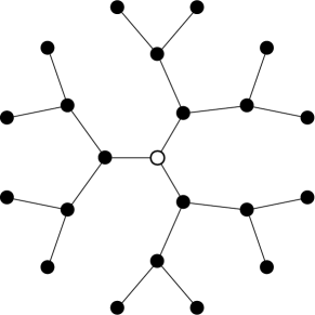
Figure 1: Cayley tree for $z=2$ and $g=3$. The root node is indicated in white.

We now compute the modularity of a specific partition of the Cayley tree, which we call the analytic partition. First place the root node into a community of its own. Then create a new community for each child of the root node, containing that child and all of its descendants. Thus there are $z+2$ communities in total. Apart from the singleton community containing the root node, every community is a complete $z$-ary tree (which is not exactly a Cayley tree) with $g-1$ generations. Partitioning the tree in this way requires cutting only $z+1$ links. There are zero links inside the singleton community and

$$m=\frac{N(g)-1}{z+1}-1=z\frac{1-z^{g-1}}{1-z}$$ (4)

links inside the $z+1$ other communities. To compute the total degree of nodes within the community, we note that all $[N(g)-1]/(z+1)$ nodes have degree $z+1$ except the $n(g)/(z+1)$ boundary nodes that have degree 1. Thus the total degree is

$$K =(z+1)\left(\frac{N(g)-1}{z+1}-\frac{n(g)}{z+1}\right)+\frac{n(g)}{z+1}$$

$$=\frac{1+z-2z^{g}}{1-z}.$$ (5)

The final modularity is then given by substituting these expressions for $m$, $K$, and $M$ into:

$$Q_{\mathrm{cayley}} =(z+1)\left[\frac{m}{M}-\left(\frac{K}{2M}\right)^{2}\right]-\left(\frac{z+1}{2M}\right)^{2},$$ (6)

where the functional dependence on $z$ and $g$ has been suppressed. For $z=10$ and $g=4$, for example, $Q_{\mathrm{cayley}}\approx 0.91$, an extremely high modularity. Even for $z=3$ and $g=3$ we have a high modularity of $Q_{\mathrm{cayley}}\approx 0.7$. (Raw modularity values must be approached with caution; we will quantify these numbers in Sec. V.) In general, the limiting value of $Q_{\mathrm{cayley}}$ for a given $z$ is

$$\lim_{g\to\infty}Q_{\mathrm{cayley}}(z,g)=\frac{z}{z+1}.$$ (7)

Even for a finite $g>1$, $Q_{\mathrm{cayley}}\to 1$ as $z\to\infty$. Thus the Cayley tree is able to achieve arbitrarily high modularity partitions. (We will later show these partitions to also be statistically significant.) This is not the only partition capable of achieving high modularity. We discuss another partition in the Appendix.

Meanwhile, the $z+1$ branch communities of the Cayley tree’s analytic partition each have conductance

$$\phi_{\mathrm{cayley}}=\frac{1}{m}=\frac{1-z}{z-z^{g}}.$$ (8)

For $z=4$ and $g=10$, for example, $\phi_{\mathrm{cayley}}\approx 2.86\times 10^{-6}$, a very small value. This makes sense since only a single link separates that entire branch from the rest of the graph. This also emphasizes that conductance is primarily a measure of bottlenecks and isolation and should be approached with caution when applied to community structure.

Finally, we remark that the partition density of the Cayley tree is zero since $m_{c}=n_{c}-1$. This is true not just for the analytic partition but for all partitions of the Cayley tree where each community is connected.

III.2 A clique and a tree

In practice, one may deal with networks with wide fluctuations in local density, meaning there may exist localized subgraphs of low and of high density at the same time. We analyze a simple example consisting of a single complete graph known as a clique connected by one link to the root of a $z$-ary tree of $g$ generations. See Fig. 2.

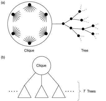
Figure 2: (a) A mixed test case consisting of a single clique (complete subgraph) of $n_{\mathrm{clique}}$ nodes connected by a single link to a $z$-ary tree. This is partitioned into communities by cutting the single bridging link. (b) A generalization where now $T$ trees are connected to the single clique ($T<n_{\mathrm{clique}}$).

We wish to compute the modularity of a community partition containing the entire clique in one community and the entire tree in the other, where only the link from the root of the tree to the clique was cut. We assume that there are $n_{\mathrm{clique}}$ nodes in the clique and $n_{\mathrm{tree}}=\left(1-z^{g+1}\right)/\left(1-z\right)$ nodes in the tree. The numbers of links in each subgraph are $m_{\mathrm{clique}}=\binom{n_{\mathrm{clique}}}{2}$ and $m_{\mathrm{tree}}={z\left(1-z^{g}\right)}/\left(1-z\right)$, respectively. The total number of links is $M=m_{\mathrm{clique}}+m_{\mathrm{tree}}+1$, and the total degrees are $K_{\mathrm{clique}}=n_{\mathrm{clique}}+(n_{\mathrm{clique}}-1)^{2}$ and $K_{\mathrm{tree}}=z^{g}+\left(z+1\right)\left(1-z^{g}\right)/\left(1-z\right)$. The final modularity of the partition is then given by substituting these expressions into

$$Q_{\mathrm{clique-tree}} =\frac{m_{\mathrm{clique}}+m_{\mathrm{tree}}}{M}-\frac{K_{\mathrm{clique}}^{2}+K_{\mathrm{tree}}^{2}}{4M^{2}}.$$ (9)

We plot Eq. (9) as a function of $g$ in Fig. 3(a) for $n_{\mathrm{clique}}=100$ and several values of $z$. We see that $Q$ attains a maximum of $1/2$, a value not as high as the pure Cayley tree previously analyzed despite the addition of a “perfect” community. We also see that, as $z$ increases, $Q$ becomes more sharply peaked as a function of $g$. This is due to the resolution limit: the larger $z$ is, the more quickly the tree will grow from one generation to the next, and thus the tree community more quickly passes beyond the size preferred by modularity. This leads to a $Q$ that grows more rapidly and then decays more rapidly as $g$ increases.

We also study a generalization of Fig. 2(a) from one tree to $T$ trees [Fig. 2(b)], where each tree is its own community. For this model $m_{\mathrm{tree}}$ and $K_{\mathrm{tree}}$ are unchanged for each tree, while now $K_{\mathrm{clique}}=T+n_{\mathrm{clique}}(n_{\mathrm{clique}}-1)$, $M=m_{\mathrm{clique}}+Tm_{\mathrm{tree}}+T$, and

$$Q_{\mathrm{clique-trees}}=\frac{m_{\mathrm{clique}}+Tm_{\mathrm{tree}}}{M}-\frac{K_{\mathrm{clique}}^{2}+TK_{\mathrm{tree}}^{2}}{4M^{2}}.$$ (10)

We plot Eq. (10) in Fig. 3(b) as a function of $n_{\mathrm{clique}}$ for several values of $T$. We see that increasing $T$ raises the overall modularity of the partition, giving apparently high values of $Q_{\mathrm{clique-trees}}>0.8$. We also see that, as $T$ increases, the curve becomes more flat, meaning that good quality partitions, according to modularity, exist for a wide range of clique sizes. We remark that this generalization may also be treated by exploiting the recursive nature of $z$-ary trees by merging all the tree roots into one node and moving that node into the clique (this is particularly simple when $T=z$).

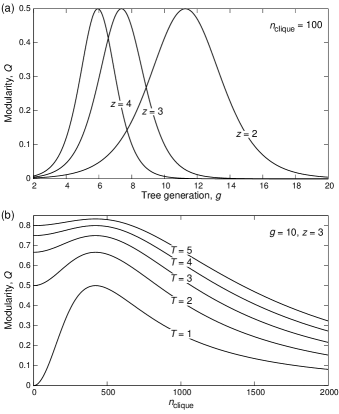
Figure 3: (a) Modularity for the example network illustrated in Fig. 2(a). As we increase the size of the tree for a fixed clique size, the modularity grows to a maximum value and then decays away. This is due to the resolution limit: there exists a specific tree size that maximizes $Q$ for each clique size. (b) For the generalization of one clique and $T$ trees, shown in Fig. 2(b), we see that the analytic partition again attains high modularity, especially as more trees are added. Likewise, as $T$ increases we see that the peak of $Q$ flattens out and that the partition has high modularity for a range of clique sizes. This means that much of the resolution limit can be compensated for if the network is sufficiently treelike.

In Sec. V we study the statistical significance of these clique-tree partitions.

III.3 Other trees

The results above were derived for Cayley and $z$-ary trees. The regular nature of these trees allows for tractable expressions of modularity, but our results are not limited to these types of trees. The important feature in this context is that all connected subgraphs of $n$ nodes in any tree will always contain $m=n-1$ links. Since it seems a reasonable basic requirement for a community detection method to discover communities that are connected, this density relation is a reasonable minimum baseline for a method to be compared against. This also means that, since every tree obeys this relation, bottlenecks become the primary drivers of high modularity partitions in all trees. We further explore the generality of our results in Sec. IV, where we apply community detection algorithms to random trees.

IV Real-world examples

The above derivations show that trees may possess arbitrarily high values of modularity. However, these calculations did not consider the resolution limit of modularity. In fact, real-world optimization of modularity will result in partitions that give even higher values of $Q$ than those of the analytic partitions discussed in Sec. III.

To see this we apply two of the most popular and successful community discovery methods. The first is known as fast unfolding (sometimes referred to as the Louvain method) and can efficiently find very high modularity partitions Blondel et al. (2008). The second method is called infomap Rosvall and Bergstrom (2008). Infomap does not optimize modularity, instead exploiting information-theoretic arguments, but the partitions it does find are often high in modularity, especially for undirected networks.

We apply these algorithms to the Cayley tree. In Fig. 4 we plot the modularities discovered by each algorithm and the modularities $Q_{\mathrm{cayley}}$ of the analytic partitions [Eq. (6)]. We see that the methods find communities that appear as strong as the analytic method or stronger. Fast unfolding typically exceeds $Q_{\mathrm{cayley}}$ as the trees grow, and even approaches $Q=1$. Infomap tends to stay closer to $Q_{\mathrm{cayley}}$, but it too can exceed these bounds, especially for trees with $z=2$. If these methods were applied blindly to a network, such high values of modularity would suggest that these communities are extremely high quality and that the network was extremely modular.

Figure 4: (Color online) Community discovery methods find even higher values of modularity than the analytical partition of the Cayley tree. We apply two methods: (a) fast unfolding Blondel et al. (2008) and (b) infomap Rosvall and Bergstrom (2008) for several values of $z$. Solid symbols correspond to Eq. (6) while open symbols correspond to the modularities found by the methods. Fast unfolding finds consistently higher modularity partitions than the analytic partition, due to the resolution limit. These partitions even approach $Q=1$. Infomap, which does not optimize modularity, tends to find partitions comparable to the analytic partition, although it too finds higher value partitions for $z=2$ and some values of $g$ for $z=3$. Note that the vertical axes do not begin at $Q=0$.

What about trees other than the Cayley tree? Will such discovery methods find comparable values of modularity? To answer this, we now apply these methods to random trees generated from a Galton-Watson branching process Harris (2002), where each node has a random number of descendants drawn from a Poisson distribution with mean $\lambda$. (We also stop growing the tree at $g$ generations.) For $\lambda=4$ and $g=6$, for example, we find fast unfolding partitions with modularity $Q=0.9814\pm 0.0055$, while for infomap we find partitions with $Q=0.8594\pm 0.0069$. This supports the generality of our results: high modularity partitions also exist in non-Cayley trees.

As a final practical example, we also apply both methods to a treelike network derived from a genealogical dataset capturing the advisor-advisee relationships between mathematicians and their students North Dakota State University ; Malmgren et al. (2010). (This genealogy is not exactly a tree since some students have multiple advisors.) We only consider the giant connected component of the network, capturing approximately $90\%$ of the dataset. In total the network has $N=133319$ nodes and $M=148247$ links. The modularities of the partitions found by fast unfolding and infomap are $Q_{\mathrm{FU}}=0.951083$ and $Q_{\mathrm{IM}}=0.877146$, respectively. These high values would again imply that the network is strongly modular; however, statistical testing should be performed to support this argument (see Sec. V).

As a brief aside, another interesting aspect of a community partition is the distribution of community sizes (numbers of nodes per community). Since any discovered modular network structure depends intrinsically on the definition at the heart of the algorithm used to find that structure, it is not known for certain what the true distribution is. Nevertheless, there has been empirical evidence showing that the size distribution may exhibit a power law $Pr(s)\sim s^{-\alpha}$, for $\alpha\geq 1$ Palla et al. (2005); Ahn et al. (2010).

Yet the distributions of community sizes found in the genealogical network, shown in Fig. 5, are not heavy-tailed. Instead both methods find approximately exponential distributions, with a small number of larger communities that would be underrepresented by an exponential distribution. The lack of very large communities may be expected in graphs without hubs, but the degree distribution for this network is heavy tailed [Fig. 5(b), inset]. This relatively narrow size distribution may provide some warning that the communities found in this network differ from typical communities in some meaningful way, though this is far from certain. Further study of this distribution may prove fruitful in understanding the modular nature of complex systems.

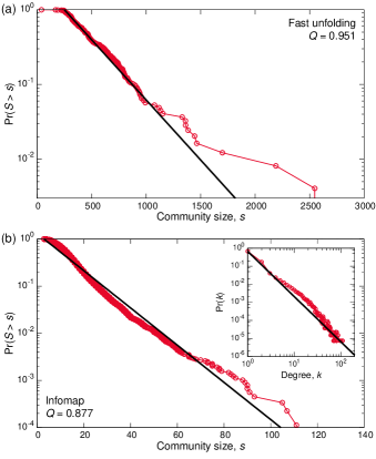
Figure 5: (Color online) The distribution of community sizes found in the genealogical network for (a) fast unfolding and (b) infomap. We see that neither distribution is heavy tailed, being instead approximately exponential (straight lines) except for a small number of the largest communities that would be underestimated by an exponential distribution. The inset shows that unlike the community size distribution, the degree distribution of the network is heavy tailed. The straight line shows a pure power law, $\mathrm{Pr}(k)\sim k^{-2.5}$, for comparison.

V Statistical testing

Given that there exist high modularity partitions in both the Cayley tree and the mathematics genealogy, a crucial question becomes, are these partitions significant in some way, or could they be simply due to some random process? This is especially important since it is known that sparse, uncorrelated graphs can potentially possess high modularity partitions due to fluctuations Reichardt and Bornholdt (2006a, b); Guimera et al. (2004). To address such questions of statistical significance requires first defining an appropriate null model. Hypothesis testing then asks what is the probability that the observed phenomena (in this case the discovered communities or their properties) may have arisen within the null model. If this probability is sufficiently low, then there is evidence that the communities cannot be explained by the null model. This does not mean that the communities are “meaningful,” however, since this only compares them to that particular null model. For example, a simple choice of null model is the configuration model: build uncorrelated random graphs that preserve the degree sequence of the original graph, apply community detection to these graphs, and then compare the configuration model communities to those of the original network. However, a Cayley tree is typically very different from its equivalent configuration model ensemble, being highly structurally ordered, and this alone may lead to statistically significant differences in, e.g., modularity. Thus it is crucial to choose the most appropriate null model possible.

Defining statistical tests for community structure remains an area of research Lancichinetti et al. (2010); Mirshahvalad et al. (2012). For our purposes, we use the testing procedure introduced in Lancichinetti et al. (2010). Roughly, this test takes the worst node $w$ in a community $c$ (the node with the least neighbors also inside $c$), removes $w$ from $c$, and asks what is the probability $p$ that $w$ would have that many neighbors or more within $c$ if its links were distributed randomly over the whole graph while holding the rest of $c$ and the degrees of all other nodes fixed. Since $w$ represents the worst case, if $p$ is small, then it is unlikely that $w$ or any other nodes in $c$ would have so many other neighbors also in $c$ due to chance. Therefore, they consider a community to be significant if $p<0.05$, the standard significance level for hypothesis testing. Note that this test strictly controls for both the links inside $c$ (and therefore its density), the number of links exiting $c$, and the overall sparsity of the network. The authors in Lancichinetti et al. (2010) used this test to show that communities in sparse Erdős-Rényi and power law graphs are not significant. For full details, see Lancichinetti et al. (2010).

Here, we compute a $p$ for each community of interest using their method and ask what fraction of communities are significant.

For the analytic partitions of the Cayley tree (Sec. III.1), we find that all $z+1$ branch communities are statistically significant. (For $z=3$ and $g=7$, for example, the maximum $p=0.00144$.) This means that this particular partition cannot be explained simply by the global sparsity of the tree itself. In particular, this test considers the internal structure of a community as fixed, and yet these communities are significant even though they are internally maximally sparse trees. This contradicts the typical intuition of communities as internally dense, externally sparse subgraphs and supports the argument that bottlenecks alone are sufficient to significantly optimize modularity.

We next test the analytic partition of the clique-tree example (Sec. III.2). We consider for $n_{\mathrm{clique}}=100$ all $z=2,3,4$ and $g=2,\ldots,10$ [see also Fig. 3(a)]. In all cases both communities were significant: the maximum $p$ observed from any combination of those parameters was $p=0.00387$.

We now turn to the community discovery methods fast unfolding and infomap. For fast unfolding on the Cayley tree ($z=3$, $g=7$) we find that approximately 91% of the discovered communities were significant. This shows that even practical methods can find statistically significant, high modularity partitions solely through the discovery of bottlenecks. For infomap, which does not optimize modularity, we find that no communities are statistically significant according to this test. However, we remark that a less strict test also introduced in Lancichinetti et al. (2010) shows that approximately 48% of the infomap communities are significant. The truth likely lies between these extremes, but we can safely conclude that most infomap communities could be explained by this test’s null model.

Next, we test fast unfolding and infomap on the finite Galton-Watson trees discussed in Sec. IV. We find comparable results to the partitions of the Cayley tree: for $\lambda=4$ and $g=6$, we find that $96.9\%\pm 0.808\%$ fast unfolding communities were significant, while almost no ($0.0311\%\pm 0.0350\%$) infomap communities were significant.

Finally, we consider the practical example of the mathematics genealogy. Both Fast unfolding and infomap found apparently high values of modularity, but are these results significant? Applying this test shows that they are not: for Fast Unfolding and infomap only approximately 2.4% and 2.6% of the communities were significant, respectively. Although we again caution that this does not necessarily prove these communities to be meaningless, it further underlines the potential danger of relying upon raw modularity values as a quantifier of modular structure.

VI Discussion and conclusions

We have shown that trees appear very modular, yet connected trees are maximally sparse and possess no density fluctuations, going against the tenet that communities are unusually dense subgraphs. Thus, counter to our intuition, measures such as modularity, while ostensibly rewarding densely interconnected groups, can actually be optimized solely through the discovery of bottlenecks, and it is not necessary for the discovered groups to be internally dense. In particular, we do not claim that trees lack communities, nor do we claim that these communities are not meaningful in some way. Instead, we argue only that it is sufficient to discover bottlenecks to optimize modularity and conductance. This disconnect between intuition and practice has not been well discussed in the literature, and in fact most work has overlooked the outsized role that bottlenecks play in the existence of modular structure.

So is our definition of modular structure correct? Equation (2) depends so strongly on its null model that we must judiciously understand all facets of it. We have shown that communities do not need a significantly high internal density to lead to high quality (according to modularity). Therefore, if researchers want to consider modules according to their intuition, they may need to introduce measures that specifically account for internal density in some way beyond that of Eq. (2). Taken together with modularity’s other issues such as its resolution limit, it appears that rigorously and unambiguously quantifying modular network structure is difficult and remains an open question.

Researchers have shown that sparse graphs will have high modularity, yet the statistical tests applied here show that the sparsity of trees alone is not sufficient to explain these results. By controlling for tree sparsity, we have shown that bottlenecks lead not only to high modularity but to statistically significantly high modularity. Our results on trees further differ from sparse random graphs in that the expected high modularity partitions do not need to be equipartitions (see Appendix), and the derivations here do not invoke features of ensembles of random graphs.

One may suspect that the addition of nontree components to a network may destroy the observed phenomena, that it is somehow fragile, yet our results in Sec. III.2 show that this is not the case and that merely the presence of trees may lead to modular structure. A crucial consequence of this is that, since trees are the limiting structure as networks become sparse, sampled and missing data Bagrow et al. may boost modularity, at least in some regions of the network, even though the network remains globally connected. Incomplete data remain an issue in high-throughput biological assays, for example Yu et al. (2008), and thus one should consider both sparsity and bottlenecks when approaching graph partitioning in these problems.

Finally, the statistical tests we used in Sec. V show that many of the communities found in trees are significant, whereas the communities found in the mathematics genealogy, while very high in modularity, are typically not significant. However, this test does not verify that the tree communities are “meaningful,” only that they differ from the test’s null model. Likewise, the discovered genealogical communities could still be meaningful in other ways, perhaps revealing important schools of mathematicians or mathematics research. For networks that possess additional data annotating the properties or roles of network elements, for example gene ontology terms describing proteins in protein-protein interaction networks Gene Ontology Consortium (2008); Gavin et al. (2006); Krogan et al. (2006); Yu et al. (2008), these discovered groups may in fact be highly enriched, meaning that their nodes or links share many annotations Ahn et al. (2010); Traud et al. (2011), even though structurally the community is not significant. Further study of the interplay between these different validation mechanisms may be crucial to increasing our understanding of modular networks and complex systems in general.

*

Appendix A Another high modularity partition of the Cayley tree

Consider the analytic partition of the Cayley tree, where the root node occupies a singleton community alongside the $z+1$ branch communities. Neglecting the singleton community, which has a vanishing contribution to $Q$ anyway, the communities are all the same size. We showed in Sec. III that the modularity of this partition $Q_{\mathrm{cayley}}$ can become arbitrarily close to $1$. This is not the only arbitrarily high modularity partition present in the Cayley tree.

To see this, take one of the $z+1$ branch communities and “shatter” it such that all nodes in that branch now form singleton communities of their own. The modularity $Q_{\mathrm{shattered}}$ of this partition is

$$Q_{\mathrm{shattered}}= ~{}z\left[\frac{m}{M}-\left(\frac{K}{2M}\right)^{2}\right]$$

$${}-\left(\frac{N(g)-1}{z+1}-\frac{n(g)}{z+1}+1\right)\left(\frac{z+1}{2M}\right)^{2}$$

$${}-\frac{n(g)}{z+1}\left(\frac{1}{2M}\right)^{2}.$$ (11)

Here the first term is the contribution of the remaining $z$ “unshattered” branches, the second term accounts for the losses due to singleton interior nodes, both the root node and the shattered branch interior, and the last term accounts for losses due to the singleton leaf or interface nodes of the shattered branch. The quantities $m$, $M$, $K$, $n(g)$, and $N(g)$ correspond to those derived in Sec. III.1. Substituting these into Eq. (11) gives

$$\lim_{g\to\infty}Q_{\mathrm{shattered}}=\left(\frac{z}{z+1}\right)^{2}.$$ (12)

As expected, this value is smaller than the limit $Q_{\mathrm{cayley}}\to z/(z+1)$ as $g\to\infty$ but it shows that this partition still achieves arbitrarily high values of modularity.

As mentioned in the main text, it has been shown that sparse, uncorrelated random graphs may possess high modularity partitions Reichardt and Bornholdt (2006b, a). Under these conditions all communities should be equivalent in expectation and thus one expects all communities to be roughly comparable in size, so that the community structure must be an equipartition of the network. The high value of modularity displayed in Eq. (12) shows that trees, while also being sparse, can contain high modularity partitions that are very far from equipartitions, in contrast to the results of Reichardt and Bornholdt (2006b, a).

References

- Newman (2010) M. E. J. Newman, Networks: An Introduction (Oxford University Press, 2010).
- Albert and Barabási (2002) R. Albert and A.-L. Barabási, Rev. Mod. Phys. 74, 47 (2002).
- Newman (2003) M. Newman, SIAM Rev. 45, 167 (2003).
- Barrat et al. (2008) A. Barrat, M. Bathélemy, and A. Vespignani, Dynamical Processes on Complex Networks (Cambridge University Press, Cambridge, 2008).
- Vespignani (2011) A. Vespignani, Nat. Phys. 8, 32 (2011).
- Onnela et al. (2007a) J.-P. Onnela, J. Saramäki, J. Hyvönen, G. Szabó, M. A. de Menezes, K. Kaski, A.-L. Barabási, and J. Kertész, New J. Phys. 9, 179 (2007a).
- González et al. (2008) M. C. González, C. A. Hidalgo, and A.-L. Barabási, Nature (London) 453, 779 (2008).
- Bagrow et al. (2011) J. P. Bagrow, D. Wang, and A.-L. Barabási, PLoS ONE 6, e17680 (2011).
- Jeong et al. (2000) H. Jeong, B. Tombor, R. Albert, Z. Oltvai, and A. Barabási, Nature (London) 407, 651 (2000).
- Milo et al. (2002) R. Milo, S. Shen-Orr, S. Itzkovitz, N. Kashtan, D. Chklovskii, and U. Alon, Science 298, 824 (2002).
- Dunne et al. (2002) J. Dunne, R. Williams, and N. Martinez, Ecology Letters 5, 558 (2002).
- Krause et al. (2003) A. E. Krause, K. A. Frank, D. M. Mason, R. E. Ulanowicz, and W. W. Taylor, Nature (London) 426, 282 (2003).
- Schulman et al. (2011) L. S. Schulman, J. P. Bagrow, and B. Gaveau, Advs. Complex Syst. 14, 829 (2011).
- Barabási and Albert (1999) A.-L. Barabási and R. Albert, Science 286, 509 (1999).
- Kleinberg (2000) J. Kleinberg, Nature (London) 406, 845 (2000).
- Colizza et al. (2006) V. Colizza, A. Barrat, M. Barthelemy, and A. Vespignani, Proc. Natl. Acad. Sci. U.S.A. 103, 2015 (2006).
- Brockmann et al. (2006) D. Brockmann, L. Hufnagel, and T. Geisel, Nature (London) 439, 462 (2006).
- Watts and Strogatz (1998) D. J. Watts and S. H. Strogatz, Nature (London) 393, 440 (1998).
- Fortunato (2010) S. Fortunato, Physics Reports 486, 75 (2010).
- Newman (2011) M. E. J. Newman, Nat. Phys. 8, 25 (2011).
- Clauset et al. (2008) A. Clauset, C. Moore, and M. E. J. Newman, Nature (London) 453, 98 (2008).
- Onnela et al. (2007b) J.-P. Onnela, J. Saramäki, J. Hyvönen, G. Szabó, D. Lazer, K. Kaski, J. Kertész, and A.-L. Barabási, Proc. Natl. Acad. Sci. U.S.A. 104, 7332 (2007b).
- Ratti et al. (2010) C. Ratti, S. Sobolevsky, F. Calabrese, C. Andris, J. Reades, M. Martino, R. Claxton, and S. H. Strogatz, PLoS ONE 5, e14248 (2010).
- Expert et al. (2011) P. Expert, T. S. Evans, V. D. Blondel, and R. Lambiotte, Proc. Natl. Acad. Sci. U.S.A. 108, 7663 (2011).
- Thiemann et al. (2010) C. Thiemann, F. Theis, D. Grady, R. Brune, and D. Brockmann, PLoS ONE 5, e15422 (2010).
- Bagrow and Bollt (2005) J. P. Bagrow and E. M. Bollt, Phys. Rev. E 72, 046108 (2005).
- Clauset (2005) A. Clauset, Phys. Rev. E 72, 026132 (2005).
- Bagrow (2008) J. P. Bagrow, J. Stat. Mech. P05001 (2008).
- Palla et al. (2005) G. Palla, I. Derényi, I. Farkas, and T. Vicsek, Nature (London) 435, 814 (2005).
- Ahn et al. (2010) Y.-Y. Ahn, J. P. Bagrow, and S. Lehmann, Nature (London) 466, 761 (2010).
- Ball et al. (2011) B. Ball, B. Karrer, and M. E. J. Newman, Phys. Rev. E 84, 036103 (2011).
- Sreenivasan et al. (2007) S. Sreenivasan, R. Cohen, E. López, Z. Toroczkai, and H. E. Stanley, Phys. Rev. E 75, 036105 (2007).
- Bollobás (1998) B. Bollobás, Modern Graph Theory (Springer, Berlin, 1998).
- Newman and Girvan (2004) M. E. J. Newman and M. Girvan, Phys. Rev. E 69, 026113 (2004).
- Newman (2004) M. E. J. Newman, Phys. Rev. E 69, 066133 (2004).
- Fortunato and Barthelemy (2007) S. Fortunato and M. Barthelemy, Proc. Natl. Acad. Sci. U.S.A. 104, 36 (2007).
- Lancichinetti and Fortunato (2011) A. Lancichinetti and S. Fortunato, Phys. Rev. E 84, 066122 (2011).
- Reichardt and Bornholdt (2006a) J. Reichardt and S. Bornholdt, Phys. D 224, 20 (2006a).
- Reichardt and Bornholdt (2006b) J. Reichardt and S. Bornholdt, Phys. Rev. E 74, 016110 (2006b).
- Guimera et al. (2004) R. Guimera, M. Sales-Pardo, and L. A. N. Amaral, Phys. Rev. E 70, 025101 (2004).
- Good et al. (2010) B. H. Good, Y.-A. de Montjoye, and A. Clauset, Phys. Rev. E 81, 046106 (2010).
- Blondel et al. (2008) V. Blondel, J. Guillaume, R. Lambiotte, and E. Lefebvre, J. Stat. Mech. 2008, P10008 (2008).
- Rosvall and Bergstrom (2008) M. Rosvall and C. T. Bergstrom, Proc. Natl. Acad. Sci. U.S.A. 105, 1118 (2008).
- Harris (2002) T. E. Harris, The Theory of Branching Processes (Dover, New York, 2002).
- (45) North Dakota State University, “The mathematics genealogy project,” http://genealogy.math.ndsu.nodak.edu.
- Malmgren et al. (2010) R. D. Malmgren, J. M. Ottino, and L. A. N. Amaral, Nature (London) 465, 622 (2010).
- Lancichinetti et al. (2010) A. Lancichinetti, F. Radicchi, and J. J. Ramasco, Phys. Rev. E 81, 046110 (2010).
- Mirshahvalad et al. (2012) A. Mirshahvalad, J. Lindholm, M. Derlén, and M. Rosvall, PLoS ONE 7, e33721 (2012).
- (49) J. P. Bagrow, S. Lehmann, and Y.-Y. Ahn, arXiv:1102.5085 .
- Yu et al. (2008) H. Yu, et al. Science 322, 104 (2008).
- Gene Ontology Consortium (2008) Gene Ontology Consortium, Nucleic Acids Res. 36, D440 (2008).
- Gavin et al. (2006) A.-C. Gavin, et al. Nature (London) 440, 631 (2006).
- Krogan et al. (2006) N. J. Krogan, et al. Nature (London) 440, 637 (2006).
- Traud et al. (2011) A. L. Traud, E. D. Kelsic, P. J. Mucha, and M. A. Porter, SIAM Review 53, 526 (2011).