Chaotic mixing and the secular evolution of triaxial cuspy galaxy models built with Schwarzschild’s method

Abstract

We use both N-body simulations and integration in fixed potentials to explore the stability and the long-term secular evolution of self-consistent, equilibrium, non-rotating, triaxial spheroidal galactic models. More specifically, we consider Dehnen models built with the Schwarzschild method. We show that short-term stability depends on the degree of velocity anisotropy (radially anisotropic models are subject to rapid development of radial-orbit instability). Long-term stability, on the other hand, depends mainly on the properties of the potential, and in particular, on whether it admits a substantial fraction of strongly chaotic orbits. We show that in the case of a weak density cusp ($\gamma=1$ Dehnen model) the N-body model is remarkably stable, while the strong-cusp ($\gamma=2$) model exhibits substantial evolution of shape away from triaxiality, which we attribute to the effect of chaotic diffusion of orbits. The different behaviour of these two cases originates from the different phase space structure of the potential; in the weak-cusp case there exist numerous resonant orbit families that impede chaotic diffusion. We also find that it is hardly possible to affect the rate of this evolution by altering the fraction of chaotic orbits in the Schwarzschild model, which is explained by the fact that the chaotic properties of an orbit are not preserved by the N-body evolution. There are, however, parameters in Schwarzschild modelling that do affect the stability of an N-body model, so we discuss the recipes how to build a ‘good’ Schwarzschild model.

1 Introduction

The Schwarzschild method is an important tool for constructing self-consistent equilibrium models of galaxies, when the system does not have an analytic distribution function (Schwarzschild, 1979). Models of triaxial galaxies are of particular interest, since they often admit a large fraction of chaotic orbits.

The aim of the Schwarzschild method is to construct self-consistent equilibrium models, in which orbits in a given potential are arranged so that the resulting density matches the potential via the Poisson equation. On the other hand, dynamical stability of these models is out of the scope of the Schwarzschild method.

There are two reasons why such a model might turn out to be non-stationary. First this could be due to dynamical instabilities, such as the radial-orbit instability (e.g. Polyachenko & Schukhman, 1981), which manifest themselves on a rather short time, typically of the order of a crossing time. The other reason concerns more gradual evolution and is related to the existence of chaotic orbits in most non-integrable potentials, especially those having a high central mass concentration (density cusp or black hole). Orbits in the Schwarzschild model (SM) are regarded as stationary ‘building blocks’, which ensures that the distribution function of the whole model satisfies the time-independent collisionless Boltzmann equation (Binney & Tremaine, 2007), $df/dt=0$. By construction, orbits are evolved for a certain time, typically of order $10^{2}$ dynamical times, which is expected to be sufficient to sample the available phase space. This is a reasonable assumption for regular orbits, which fill their invariant tori more or less uniformly during this time. But chaotic orbits have a much larger region of available phase space (of higher dimensionality) and may sample it in a very non-uniform way, remaining in a confined portion of this region for many hundreds of dynamical times. This may lead to the effect of chaotic diffusion, when these orbits eventually escape to a different region of phase space and, accordingly, change their shape in configuration space, which leads to the breakdown of the self-consistency of the model.

The stability of models built with Schwarzschild’s method has been tested by N-body simulations as early as in Smith & Miller (1982), albeit with a rather rough N-body code and on a short timescale. Zhao (1996) confirmed the stability of a galactic bar model using the self-consistent field (SCF) method. More recently, Antonini et al. (2009) showed that the radial-orbit instability (ROI) exists also in triaxial systems, if the velocity anisotropy coefficient $\beta\gtrsim 0.3$. Wu et al. (2009) explored the existence and stability of triaxial Dehnen models in MOND gravity and found it to be acceptable. Nevertheless, their N-body models initially displayed some evolution towards a more equilibrium configuration, presumably due to difficulties associated with constructing self-consistent models in MOND gravity.

On the other hand, the effect of chaotic diffusion on the evolution of a SM is usually assumed to lead towards a more spherical mass distribution. Support for this conjecture comes from the fact that the ‘average’ shape of a fully chaotic orbit (which fills almost ergodically the equipotential surface, excluding the parts of phase space occupied by regular orbits) is generally rounder than the equidensity surface. Schwarzschild (1993) confirmed this effect for a scale-free logarithmic potential, corresponding to a $\gamma=2$ density cusp, by creating a self-consistent SM and then following the ensemble of orbits for an interval of time three times longer than was used in creating the model. He recorded the shape obtained from the superposition of these orbits for this longer interval and concluded that it was evolving towards sphericity, but that this change was quite small.

A number of studies used N-body simulations to address the long-term stability of triaxial models created by various methods, and their evolution caused by chaotic orbits. Holley-Bockelman et al. (2001) constructed an equilibrium triaxial model with axial ratio $a:b:c=1:0.85:0.7$ based on the spherical Hernquist model ($\gamma=1$) by applying artificial squeezing along two axes, and evolved it with a SCF N-body code for $\sim 8$ half-mass dynamical times to confirm that there is no significant change in shape.

Later, Holley-Bockelman et al. (2002) extended their study to include a supermassive black hole with mass $M_{\bullet}$ equal to 0.01 of the total model mass. The growth of this central point mass destabilizes the population of box orbits and converts most of them into rather strongly chaotic ones, which, in turn, quickly drives the inner regions of the model towards almost spherical shape. Again using SCF N-body code, Kalapotharakos et al. (2004) explored the dependence of such evolution on the black hole mass, and found that in all cases there existed a large fraction of chaotic orbits, but the overall shape of the model substantially evolved only for $M_{\bullet}>0.005$, when these orbits were more strongly chaotic (as measured by Lyapunov exponents), while smaller $M_{\bullet}$ did not cause much secular evolution. Muzzio et al. (2009) created a strongly triaxial model with a $\gamma\simeq 1$ cusp by cold collapse and confirmed its stability by quadrupolar (a restricted variant of SCF) N-body code over several hundred crossing times, despite having large ($\gtrsim 50\%$) fraction of chaotic orbits. All these results are based on N-body modelling, and the methods used for creating their initial conditions cannot make a system with predefined properties, unlike the iterative method of Rodionov et al. (2009), discussed in Section 7.

Poon & Merritt (2004) constructed models for triaxial scale-free cusps with $\gamma=1$ and $\gamma=2$ around a black hole using the Schwarzschild method. Their solutions contained about half of the mass in chaotic orbits, but nevertheless were found to be reasonably stable when evolved by an N-body tree-code during $6\,T_{dyn}$ (measured at few times the black hole influence radius), except for prolate ($T=0.75$) models. They conclude that their chaotic orbits were sufficiently mixed during the $T=100$ orbital times used for integration in SM, so that they represented reasonably stationary building blocks. However, the time interval was quite short (only a few dynamical times for orbits outside the radius of influence, where most chaotic orbits are found), and the change of axial ratios was small yet non-negligible. In addition, they followed the evolution of models in a fixed smooth potential for $\sim 100$ dynamical times, and found no change in shape, as is reasonable to expect, given that orbits in the SM were evolved for a similar time. Another reason for the less apparent shape evolution in their models is that for scale-free potentials the equipotential surface is not much rounder than the equidensity surface, so even ‘fully chaotic’ orbits do support the necessary model shape to some degree.

A somewhat different issue is addressed in Valluri et al. (2010). They investigated the change of shape of triaxial dark matter halos in response to the growth of a compact mass in the centre, that is, due to an adiabatic change of the potential. They compared the orbit population of the models before the growth of the central mass, after the growth (intermediate stage), and after an adiabatic ‘evaporation’ of this mass (final stage). They used an N-body tree-code both to follow the evolution of the ‘live’ system and to analyze the properties of the orbits in the ‘frozen’ N-body potential. Valluri et al. (2010) found that, in the case with no strong central mass concentration, the evolution of orbit shapes is mostly reversible, despite the fact that many of the orbits are chaotic in the intermediate stage, and attributed this reversibility to resonant trapping of orbits in the course of the slow change of the potential.

We continue and extend these studies in two interconnected aspects. Namely, we perform N-body simulations of triaxial cuspy Dehnen models built with the Schwarzschild method, and find that, in the cases when there is no rapid onset of radial-orbit instability, they are remarkably stable over many dynamical times. There is, however, a long-term evolution of the shape of these models and we find that it is caused by the influence of chaotic orbits.

We begin by introducing our triaxial Dehnen models constructed with the Schwarzschild method, and briefly review their properties in section 2. Then in section 3 we review the concept of chaos, in particular, the distinction between regular, weakly (sticky) chaotic and strongly chaotic orbits, and the quantities that are intended to represent chaotic properties of an individual orbit.

The long-term evolution of orbits in a fixed potential is the subject of section 4. It turns out that in the potentials considered here, most chaotic orbits are in fact quite sticky, and the timescale for chaotic diffusion and the associated change of orbit shapes is rather long, of order $10^{3}$ dynamical times. However, in the strong-cusp model and in the outer parts of the weak-cusp model this stickiness is less prominent, and the chaotic orbits do exhibit evolution towards a more spherical shape. We also discuss how our findings can be explained by the amount of ‘complexity’ of the phase space, that is, the presence and importance of resonant orbit families.

Next, we describe our N-body experiments which basically confirm the expectations derived from the fixed-potential evolution (section 5). Unless the velocity anisotropy in the model is sufficiently biased towards radial velocities to allow for a rapid development of the radial-orbit instability, the shape of the density distribution in the N-body model (NM) remains in agreement with that of the original Schwarzschild model (SM) for a long time. The weak-cusp model is essentially stable over the course of the simulation, while for the strong-cusp case there is a gradual evolution towards a more spherical (or, rather, oblate axisymmetrical) shape, which we attribute to chaotic diffusion.

In addition, a very important, and somewhat disappointing, finding is that we are hardly able to control the degree of evolution due to this chaotic diffusion by altering the properties of the SM. This is because the orbits in the NM, while basically resembling their counterparts in the SM in shape and orbital class, do not inherit the attribute of chaoticity from the smooth-potential model. This argues that the overall evolution of the NM is determined mostly by the gross properties of the potential, rather than by any specific arrangement of orbits (as long as this satisfies self-consistency). Nevertheless, we do present recipes for building better SM (in the sense that the corresponding NM are more stable) in section 6.

In section 7 we compare the evolution of models built with the Schwarzschild method with that of a model constructed with the iterative method (Rodionov et al., 2009), which is completely different from the SM as it relies on the ‘guided evolution’ of an N-body model towards a specific equilibrium. We show that, despite conceptually being very different, they perform similarly in terms of stability of the resulting model, and have similar properties of ensemble of orbits.

Finally, we present our conclusions.

2 Schwarzschild models

In this paper we restrict our attention to non-rotating three-dimensional systems with mild flattening. Namely, we consider two variants of the triaxial Dehnen model, with density profile

$$\rho(r)=\frac{(3-\gamma)M}{4\pi abc}\frac{1}{m^{\gamma}(1+m)^{4-\gamma}},$$ (1)

where $m=[(x/a)^{2}+(y/b)^{2}+(z/c)^{2}]^{1/2}$ is the elliptic radius. We adopt dimensionless units in which $M=1$, $a=1$, $G=1$ (which also fixes the time unit), and choose the axial ratios $b/a=\sqrt{5/8}\approx 0.79$, $c/a=1/2$, which corresponds to a triaxiality parameter $T=(a^{2}-b^{2})/(a^{2}-c^{2})$ equal to $1/2$ (maximal triaxiality). For the cusp slope $\gamma$ we choose two values: $\gamma=1$ (weak cusp) and $\gamma=2$ (strong cusp). It turns out that there are substantial differences between the two models, which will be discussed in the following sections.

All integration times and orbit frequencies in the SM are measured in units of dynamical time $T_{dyn}(E)$, which is defined as the period of the long-axis orbit with the given energy: $T_{dyn}=4\int_{0}^{r_{max}(E)}[2(E-\Phi(r))]^{-1/2}\,dr$. Other papers often use the period of the $x-y$ plane closed loop orbit, which is somewhat shorter, but our definition has the advantage that all natural frequencies of orbits are greater than $T_{dyn}^{-1}$. For our models $T_{dyn}(r)$ may be approximated as $4.4(r^{1/2}+r^{3/2})$ for the weak-cusp case and $4.4(r^{2}+r^{3})^{1/2}$ for the strong-cusp case, where time and length units are dimensionless time units.

The models were constructed using 50 radial shells, 2400 grid cells and $3\cdot 10^{4}$ orbits evolved for 500 dynamical times. The initial conditions for the orbits were assigned randomly using the following recipe: sample the elliptical radius uniformly in the value of enclosing mass, randomly choose angles to put the orbit onto the equidensity ellipsoid, and assign each component of the velocity according to a Gaussian distribution with the dispersion of the equivalent spherical model. This is different from the traditionally used method of sampling initial conditions at a small number of energy levels and in fixed positions on the grid; we find that a random position and, more importantly, continuous distribution in energy yields better models.

In the following three sections we will discuss mainly one variant for each model, namely the ‘unconstrained’ variant with no restrictions on the orbit population or on the fraction of chaotic orbits, and with a velocity anisotropy $\beta=1-\frac{\sigma_{t}^{2}}{2\sigma_{r}^{2}}$ (Binney & Tremaine, 2007) varying from 0 in the centre to $\sim 0.6$ in the outer parts. We consider the effect of variation of these parameters in section 6.

3 General remarks on the chaotic properties of an orbit

There are several methods for quantifying the degree of chaoticity of a given orbit, which may be classified into two broad groups. One group deals with a single orbit and considers its spectrum, that is, the Fourier transform of some quantity along the trajectory (e.g. the $x$ coordinate, or the distance from the centre) sampled at equally spaced moments of time. It is based on the fact that all regular orbits are multiply-periodic, with their spectra containing in 3D only linear combinations of no more than three fundamental frequencies, these frequencies being constants of the motion in a time-independent potential. Any deviation from this simple spectrum is an indication of chaos. A quantitative estimate of chaos may be obtained either as the number of spectral lines containing a specified fraction (say, 0.9) of the total power (Kandrup et al., 1997), or as the variation in these fundamental frequencies calculated e.g. from the first and second halves of the integration time (Laskar, 1993; Valluri & Merritt, 1998), dubbed ‘frequency diffusion rate’ (FDR).

The second group of methods considers the deviation of nearby orbits; the orbit in question is accompanied by one or more adjacent orbits, and the evolution of deviation vectors is tracked. In the case of a regular orbit these deviation vectors should grow no faster than linearly, and if more than one such vector is considered, they should remain correlated in direction. Conversely, in the chaotic case the deviation starts to grow exponentially after some time. This class includes methods based on the calculation of Lyapunov exponents $\Lambda$ and alignment indexes (e.g. Skokos, 2010). There is quite a good correspondence between FDR and $\Lambda$ as chaos indicators in a smooth potential. To construct SM with different fraction of chaotic orbits (Section 6), we use here the Lyapunov exponents to distinguish between regular and chaotic orbits.

For an N-body system, however, all trajectories have large positive Lyapunov exponents. Their timescale for exponential deviation is a fraction of the crossing time, and furthermore, they do not decrease with increasing $N$ (Kandrup & Sideris, 2001; Sideris & Kandrup, 2002; Valluri & Merritt, 2000). This does not preclude a more regular behaviour of the system with more particles, since Lyapunov exponents, by definition, measure the growth rate of infinitely small perturbations, but do not tell by what distance two nearby orbits will be separated after a finite time. It appears that if the phase space has a complex structure of stable resonant islands, then chaotic orbits usually tend to be confined to small regions of the entire phase space, demonstrating the so-called phenomenon of stickiness, and resemble regular orbits for many dynamical times (e.g. Contopoulos, 1971, 2002; Valluri & Merritt, 2000; Harsoula & Kalapotharakos, 2009).

Therefore, for the purpose of comparing the chaotic properties of orbits evolved in a smooth potential and in an N-body model, we will restrict ourselves to the first class of chaos detection methods. Namely, we use the following definition for the frequency diffusion rate (FDR):

$$\Delta\omega\equiv\frac{1}{3}\sum_{i=1}^{3}\frac{|\omega_{i}^{(1)}-\omega_{i}^{(2)}|}{(\omega_{i}^{(1)}+\omega_{i}^{(2)})/2}$$ (2)

Here $\omega_{i}^{(1)}$ and $\omega_{i}^{(2)}$ are the leading frequencies in Cartesian coordinates ($i=x,y,z$) for the first and the second halves of the integration time, respectively. We adopt $\Delta\omega=10^{-3}$ as the threshold separating regular from chaotic orbits, which roughly corresponds to the distinction based on the Lyapunov exponent, if both are measured on the interval of $100\,T_{dyn}$.

Unfortunately, FDR itself is not a strictly defined quantity: if we measure $\Delta\omega$ for two successive integration intervals, or even for a somewhat different duration of time (say, 100 and 110 $T_{dyn}$), or change the sampling rate, this quantity may change by a factor of few. This is not surprising, since this quantity by definition measures the difference in two ’instantaneous’ values of a fluctuating variable $\omega$, and is itself a random quantity with an uncertainty of about $0.3-0.5$ orders of magnitude.

The shape of an orbit in configuration space may be described by its inertia tensor components,

$$I_{ij}\equiv\frac{1}{N_{s}}\sum_{n=1}^{N_{s}}x_{i}^{(n)}x_{j}^{(n)}\,,$$ (3)

where $x_{i}^{(n)}$ is the $i$-th component of the $n$-th sampling point of the trajectory. If we consider only diagonal components, $\sqrt{I_{ii}}$ gives an estimate of the extent of this orbit in the $i$-th coordinate. Likewise, the quantities

$$S_{i}\equiv\frac{I_{ii}}{I_{xx}+I_{yy}+I_{zz}}\;,\quad i=x,y,z$$ (4)

describe the orbit shape (flattening in the $i$-th direction). Tracing their change over time may be used to estimate the shape evolution.

Finally, it is necessary to note that the accuracy of determination of orbital frequencies is limited by the accuracy of energy conservation (typically $\Delta\omega\simeq|\Delta E/E|$). While this is not a limitation in the case of a smooth time-independent potential (the error in energy conservation in the integrator is $\lesssim 10^{-9}$), it becomes a major obstacle when we come to analyzing the orbits in a live N-body simulation, where particles experience random variations in energy, e.g. due to two-body relaxation.

4 Secular shape evolution induced by chaotic orbits

The construction of equilibrium models by the Schwarzschild method relies on finding time-independent ‘building blocks’ as required by Jeans’ theorem. Regular orbits obviously satisfy this requirement (as long as we ensure sufficiently uniform coverage of the invariant torus), but for chaotic orbits it’s not the case. It has been suggested that all chaotic orbits of a given energy may be in fact considered as representatives of one ‘super-orbit’ (in 3D, the chaotic part of the phase space at a given energy is one interconnected region, the so-called Arnold web), and hence, if we average all these orbits, the resulting building block may also be used as a time-independent unit. In practice, however, the usefulness of this approach is doubtful, for a number of reasons. First of all, it is not easy to distinguish unambiguously regular from chaotic orbits, because some chaotic orbits may be extremely sticky and conserve their shape and frequencies over many orbital periods. Secondly, such ‘fully mixed’ models, in which all chaotic orbits with the same energy are averaged, cannot be built self-consistently (Merritt & Fridman, 1996; Siopis, 1999): the resulting super-orbit is featureless and rounder than the density distribution, and therefore not very suitable for the model, but regular orbits alone do not have a sufficient variety to support the shape, especially in the outer parts of Dehnen models.

If, on the other hand, we choose to treat chaotic orbits in the same way as regular ones in constructing SM, the model is no longer guaranteed to be stationary. It means that even in a constant potential, the shape of the mass distribution of a given chaotic orbit may slowly evolve in time, in the process of chaotic diffusion. This should lead to a global evolution of the model shape, but it is not easy to predict how strong this will be and in what sense.

In general, we may expect that a fully chaotic orbit fills all available configuration space within its corresponding equipotential surface, which is rounder than the equidensity surfaces of the triaxial model. If we somehow divide all orbits into three classes – regular, sticky and fully chaotic – then in the course of time there will be exchange of orbits between the last two classes: some sticky orbits may eventually become unstuck, and vice versa. The outcome of this ‘diffusion’ depends on the initial orbit population of the model: if initially there were few strongly chaotic orbits (which is to be expected in a triaxial self-consistent model, since such models are not very suitable to support the shape of the density distribution), then we may expect that their fraction increases in time, and the overall shape becomes rounder. However, the timescale for this chaotic mixing may be rather long, and the change of the overall shape of density distribution does not necessarily happen on this timescale. Merritt & Valluri (1996) find that an ensemble of points initially confined to a small region in the chaotic part of the phase space evolves to a nearly time-invariant mixed distribution in $\sim 100\,T_{dyn}$. However, such mixing does not necessarily distribute orbits uniformly over all the accessible chaotic part of phase space – it may well be confined to a region surrounded by resonant tori, which significantly slow down further diffusion (Valluri & Merritt, 2000).

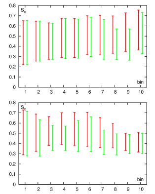
Figure 1: Shape change for chaotic orbits during $T=1000\,T_{dyn}$. Each pair of error bars shows the spread in distribution of the $x$-axis flattening $S_{x}$ (Eq. 4) for initial (left, red) and final (right, green) $100\,T_{dyn}$ intervals of time, averaged over the ensemble of chaotic ($\Delta\omega>10^{-3}$) orbits in a given energy bin. The horizontal axis corresponds to 10 bins, each of which contains 10% of the total mass, with the innermost particles in the left bin.
Top panel: $\gamma=1$, bottom: $\gamma=2$ models. The decrease in the average value in each pair means that orbits become rounder (both $y$- and $z$-axis components increase at the expense of $x$-axis component). It is evident that in the weak-cusp case only the chaotic orbits in the outer shells do change shape systematically to become rounder, while in the strong-cusp case this tendency exists for most of the radial shells.

To study this further we perform the following experiment: we create N-body realizations of SM with $10^{4}$ equal-weight particles representing a self-consistent solution, in which orbits were integrated for $100\,T_{dyn}$, Then we continue to evolve them in the same potential for 10 subsequent intervals of $100\,T_{dyn}$, and compare the properties of each orbit in the first and the last interval. The results show that indeed the chaotic orbits show the tendency to become rounder. We may quantify this by measuring the change in flattening of an orbit in each direction by using $S_{i}$ (eq. 4). Fig. 1 shows the mean value and spread of flattening along the $x$ axis, measured for the first and the last interval of $100\,T_{dyn}$, averaged over the ensemble of chaotic orbits (defined as those that changed their leading frequencies by more than $10^{-3}$ between these two intervals, as described in Sect. 3). The systematic decrease of the $x$-flattening (and corresponding increase in both $y$ and $z$, not shown here) means that orbits, on average, become rounder. But it is important to note that this effect is not observed for all energies: in the weak-cusp case, only the chaotic orbits in the outer $\sim 25\%$ of energy bins were found to exhibit a substantial evolution, while for the strong-cusp case most chaotic orbits became rounder.

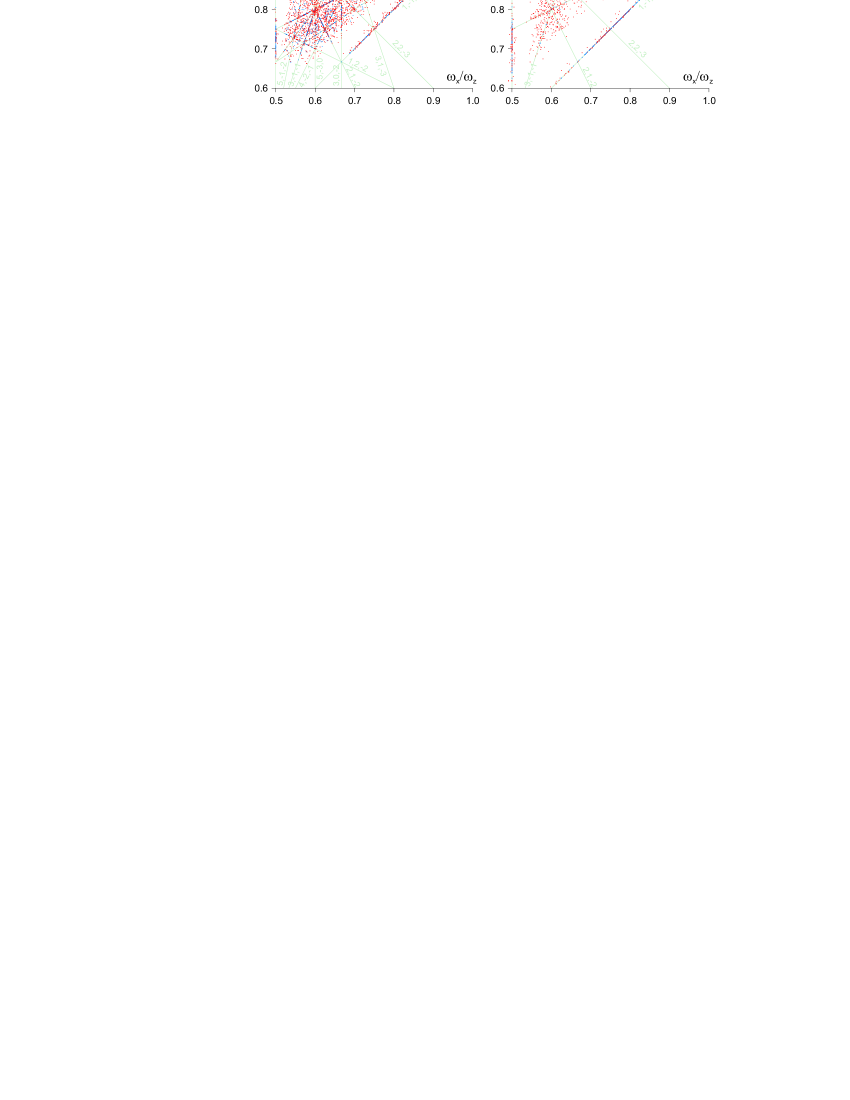
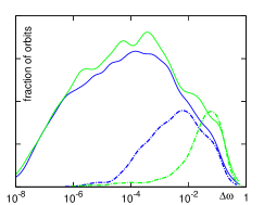
Figure 2: Frequency maps for the $\gamma=1$ (left) and $\gamma=2$ (middle) model. Blue dots mark regular and red dots chaotic orbits (as distinguished by the value of Lyapunov exponent). The right panel shows the FDR distribution ($\Delta\omega$) for these two cases (blue – $\gamma=1$, green – $\gamma=2$), separately for tube-like orbits (short axis tubes, long axis tubes and chaotic orbits close to $1:1$ resonances, solid lines) and for box-like orbits (dot-dashed lines).

The difference between these cases may be attributed to the presence of a rich network of resonances in the $\gamma=1$ model. Fig. 2 shows frequency maps for the two models. In the weak-cusp model there is a considerable fraction of points lying on or near resonant lines, corresponding to either regular or sticky chaotic orbits. Consequently, they have rather low values of FDR (right panel, blue), with $\Delta\omega\lesssim 10^{-2}$. On the other hand, $\gamma=2$ model, as well as the outer parts of $\gamma=1$ model, have no major resonances (apart from 1:1 $x-$ and $z-$axis tubes and 1:2 $x-z$ banana orbits). Most non-tube orbits in these cases are quite strongly chaotic with $\Delta\omega\gtrsim 10^{-2}$. We may thus infer that indeed the existence of resonances slows down chaotic diffusion.

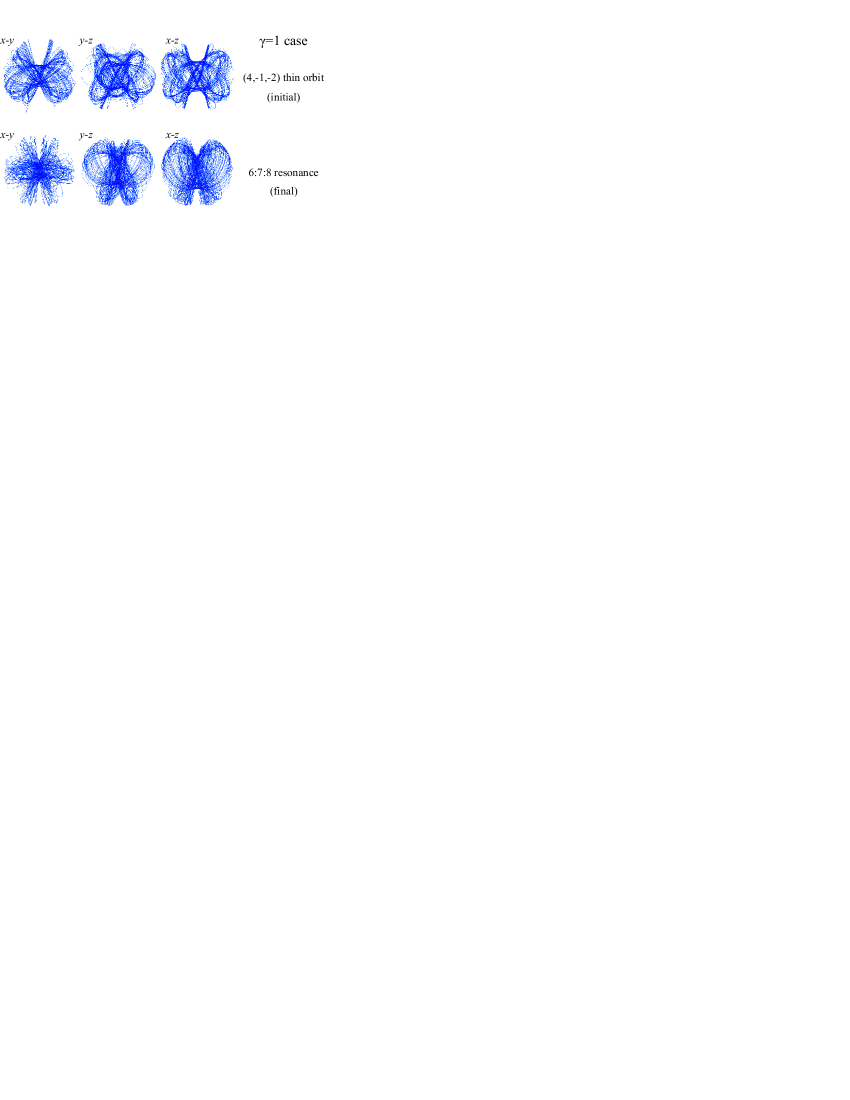
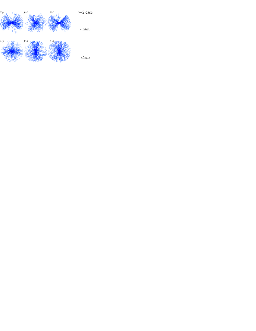
Figure 3: An example of shape change for two $100\,T_{dyn}$ segments (separated by $1000\,T_{dyn}$) of the same chaotic orbit.
Top two rows: orbit with energy from the 2nd out of the 10 bins, in the weak-cusp model. The initial and final orbit segments are parented by different resonances and have rather well-defined shapes. Even though the change in shape is substantial, there may well exist another orbit in the self-consistent solution which changes in the opposite sense.
Bottom two rows: orbit with an energy from the 9th bin in the strong-cusp model. The initial shape is more elongated along the $x$ axis, but the final one fills almost all the equipotential surface, which is close to a sphere. There were no or very few such round orbits which could become elongated to counteract this diffusion.

However, it may also be considered somewhat differently, as sketched in Fig. 3. Examination of the shapes of low-energy chaotic orbits of the $\gamma=1$ model reveals that they are mostly sticky, having a more-or-less well defined shape for any interval of $100\,T_{dyn}$. This means that even if an orbit is scattered to a different region of phase space, it may still retain a distinct shape and so represent useful ‘building blocks’. It could be expected that there is roughly a balance between orbits which became rounder and those which became flatter. On the other hand, orbits from the high-energy part of the $\gamma=1$ model are initially closer to having a well-defined shape, but become more fuzzy-looking at the end. They are not balanced by the opposite flux of orbits becoming more regular, since there were initially very few of those near-round chaotic orbits in the self-consistent equilibrium. A similar argument is used in Muzzio et al. (2005) and in Aquilano et al. (2007) to explain why it is advantageous to have a density model which is less triaxial in the outer parts, and therefore can adopt a large initial fraction of fully chaotic (almost round) orbits to balance this ‘puffing up’ of initially more elongated chaotic orbits. Anyway, the existence of shape-supporting resonances with their associated families of orbits, even chaotic, seems to be an important condition for slowing down chaotic diffusion.

On the other hand, orbits with $\Delta\omega<10^{-3}$ did not substantially change their shape in either case, neither individually, nor on average.

Up to now we considered the evolution in shape during a period of a fixed number of dynamical times, i.e. a time which varies strongly with energy. We may instead focus on the changes that may occur to the model during a fixed physical time (say, 1000 dimensionless time units, which roughly corresponds to the Hubble time and to the time of the N-body simulation which we will discuss in Sect. 5). For the weak-cusp case the dynamical time of orbits at the energies where changes in shape occur is $T_{dyn}\gtrsim 50$; hence the chaotic diffusion occurring on timescales $\gtrsim 100\,T_{dyn}$ is essentially non-relevant on the timescale of the calculation. However, for the strong-cusp case the orbits in the inner bins have $T_{dyn}\lesssim 1$, so we may expect the chaotic diffusion to have an impact on the shape evolution.

To quantify the impact that chaotic diffusion may have on the shape of a model, we used the following approach. We took the same set of $10^{4}$ orbits from a self-consistent solution as above, and re-integrated them in two variants of fixed (time-independent) potential: a smooth Dehnen analytic potential (same as was used in SM) and a frozen-N-body potential obtained from a rigid distribution of $10^{6}$ particles representing the density of the Dehnen model. We calculate the orbits for 10 subsequent intervals of time, 100 time units each (not to be confused with $100\,T_{dyn}$ in the previous experiment!). On each of these intervals, we sample 100 points from each orbit, thereby creating an N-body model with $10^{6}$ particles, and record the shape of this model. The difference from the previous experiment is that we evolved the orbits for fixed ‘physical’ time, rather than for fixed number of dynamical times which depend on energy. This way, the inner parts were much ‘older’ in terms of dynamical time.

The results of this calculation are presented later in Section 5, for the $\gamma=2$ case only. They show that evolution of shape during 1000 time units is substantial, and comparable to the evolution exhibited in the self-consistent N-body simulation. For the $\gamma=1$ case, no evolution was observed, as expected from the above consideration.

There are obvious ways to suppress this chaotic diffusion in SM. First of all, one may reduce the fraction of chaotic orbits by assigning them a penalty in the objective function. The difficulty lies in the poorly defined distinction between regular and sticky orbits, and a small fraction of (weakly) chaotic orbits in the model is unavoidable.

Second, we deliberately chose a rather small interval of integration ($100\,T_{dyn}$) for SM, which is not enough to ensure that chaotic orbits uniformly fill their allowed region of phase space. Indeed, a method proposed by Pfenniger (1984) consists in an adaptive selection of the integration time for orbits that seem to be chaotic, to improve the coverage of the available phase space: if the cell occupation numbers differ too much for the first and the second halves of the orbit, we continue the integration. The convergence, however, is not guaranteed, and can be rather slow, so one should impose an upper limit for integration time. Capuzzo-Dolcetta et al. (2007) found that even setting the maximum time equal to $2\,T_{Hubble}$ and then continuing the integration of orbits until $5\,T_{Hubble}$, some change of the overall shape of density distribution is observed.

Third, part of the problem with chaotic orbits lies in their stickiness, which may be reduced at the stage of orbit integration by adding a weak noise (random force) to the equations of motion. Kandrup et al. (2000) and Siopis & Kandrup (2000) demonstrated that even a weak noise may dramatically increase the rate of chaotic diffusion.

These efforts, however, are pretty much useless when we are trying to suppress the chaotic diffusion in an N-body model, since we found it very difficult, if at all possible, to preserve the attribute of chaoticity in transferring orbits to a slightly different potential.

5 $N$-body evolution of models

In order to confirm our expectations about the chaotic diffusion, and to test the overall stability of triaxial Dehnen models, we convert our Schwarzschild model (SM) to an N-body model (NM) by sampling points randomly from trajectories, their number being proportional to the weight of the orbit in the SM. Our standard number of bodies in NM is $10^{6}$, which means that, on average, an orbit from SM with nonzero weight is sampled with $\sim 10^{2}$ points.

We use the N-body code gyrfalcON (Dehnen, 2000, 2002) to evolve NM for $T=1000$ N-body time units, corresponding roughly to a Hubble time ($10^{10}$ yr) for a model scaled to $M=3\cdot 10^{11}\,M_{\odot}$, $a=5$ kpc. (The half-mass (long-axis) radius of the $\gamma=1$ model is $2.4$ and the dynamical time for this radius is $23$ time units; for $\gamma=2$ these values are $1$ and $6.1$, respectively). The smoothing length was set to $\epsilon=0.01$.

First we consider only one variant of the SM, namely with both the fraction of chaotic orbits and the velocity anisotropy being unconstrained. Other possibilities will be considered in section 6.

All models were initially in virial equilibrium (virial ratio $2T/W=1$ within a fraction of percent accuracy), and the kinetic and potential energy remained the same in the course of evolution to within few $\times 10^{-3}(10^{-2})$ in the weak (strong) cusp case. To check the stability of our model, we measured the change in time of the following parameters:

• mean-square change of energies of particles, to quantify the effect of two-body relaxation;

• density profile (spherically averaged);

• axial ratios of equidensity surfaces depending on radius;

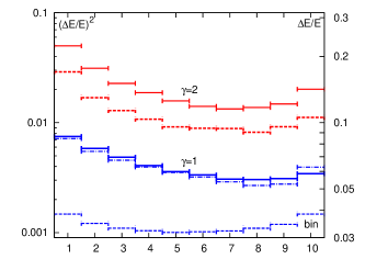
Figure 4: Relative energy change, $\Delta E/E$, after $T=1000$, for particles in 10 energy bins of N-body models (leftmost are the most bound particles). The red lines correspond to $\gamma=2$ models: the solid for $N=10^{6}$ and the dashed for $2\cdot 10^{6}$. The solid and dashed blue lines correspond to a $\gamma=1$ model, with $N=10^{6}$ and $5\cdot 10^{6}$, respectively. The blue dot-dashed line corresponds to a $N=10^{6}$ model built by the iterative method (Sec. 7).

Figure 5: Correspondence between orbits in SM and in NM, for a sample of 2000 orbits in the inner 40% of the weak-cusp model, which had completed at least 50 periods during the run.
Top panel: correlation between orbit shapes (more specifically, flattening along the $y$ axis); the shapes of the orbits in the N-body run are reasonably similar to those of the parent SM orbits.
Bottom panel: correlation between FDR – meant to measure the degree of chaos – for the two sets of orbits. Note the difference in scale between the ordinate and the abscissa. In NM the change of orbit frequencies is caused mostly by fluctuations in energy (see Fig. 7), and so has essentially no correlation with either the true degree of chaos, or the $\Delta\omega$ of the parent orbit in SM. Almost all orbits in NM have $\Delta\omega>10^{-3}$, i.e. above the threshold used for separating regular from chaotic orbits in the smooth potential.

Figure 6: Correspondence between orbits in SM (smooth) and frozen-N-body potential, for the same sample as in Fig. 5.
The top panel displays a correlation between orbit shapes, and shows that orbits in the frozen-N-body potential resemble their counterparts in the smooth potential quite well.
The bottom panel displays a similar correlation, but now between the FDR. Orbits that were regular in the smooth potential (i.e. had $\Delta\omega<10^{-3}$), have systematically a lower FDR in the frozen potential, although this rarely gets below $10^{-3}$. This is due to the graininess of the potential and not to an energy error, which is still an order of magnitude lower.

5.1 Energy change of individual particles

First we focus on the energy change of individual particles, which can be due to two effects. One is the non-stationarity of the gross potential. This, in turn, may be either due to the model being initially not in perfect equilibrium, or due to large-scale dynamical instabilities. Although the Schwarzschild modelling technique is aimed at constructing models in equilibrium, the actual accuracy of this equilibrium may vary. In particular, we found that the standard practice of assigning initial conditions for orbits from a grid of discrete energy levels results in quite large initial fluctuations of energies. We therefore adopted a smooth energy distribution for orbits in the SM. Nevertheless, the change of energy that is due to the fact that the model is not in perfect equilibrium initially should be confined to the initial times of the simulation and thus should not influence the following discussion.

The second reason for an energy change is the unavoidable two-body relaxation. It leads to a random-walk in energy space, with a mean squared deviation of energy $\Delta E^{2}$ growing linearly with time. To estimate the importance of this effect, we measured the squared relative change in energy, $(\Delta E/E)^{2}$, accumulated by the end of the integration time and averaged over particles in several energy bins (we checked that it indeed grew linearly with time, as expected for diffusion, apart from a possible initial period of faster growth if the model was not in perfect equilibrium). Figure 4 shows that this change remains quite low for the weak-cusp model, of order $|\Delta E/E|\sim$ few percent, weakly depending on the initial energy. In the strong-cusp case, the relaxation rate is $\sim 5$ times stronger, although the simulation time is still much shorter than the relaxation time for all energies.

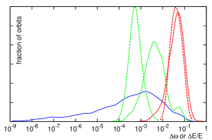
Figure 7: Histograms of FDR ($\Delta\omega$, solid lines) and of energy conservation error ($\Delta E/E$, dashed lines) for orbits from Figs. 5 and 6. The blue line corresponds to orbits in the smooth potential, green one to orbits in the frozen-N-body potential, and the red line to orbits in the live simulation.
For the live simulation the energy conservation error is quite large, between $10^{-2}$ and $10^{-1}$, and it determines the error in the frequency estimation. For the frozen-N-body potential the energy conservation is still far from being perfect (of order $\sim 10^{-4}..10^{-3}$, due to the approximations of the tree-code and the finite number of particles), but good enough not to be the major source of frequency diffusion.

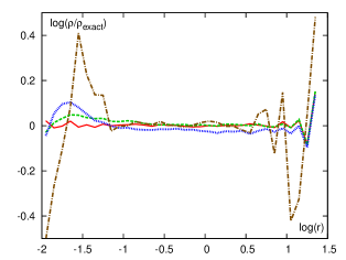
Figure 8: Density profile evolution for the $\gamma=2$ model. We plot the difference between density in the model and the exact value ($\log(\rho/\rho_{exact})$) as a function of radius ($\log(r)$). The red solid curve corresponds to the initial model, which is fairly close to the exact Dehnen profile and the green dashed curve corresponds to the model after it evolved over 10 time units. From the latter we see that the smoothing reduces the density at $r\lesssim\epsilon$ and distributes the excess of mass slightly further from centre. The blue dotted line corresponds to the end of simulation, where the axial ratios have changed substantially. For comparison, the brown dot-dashed line gives the initial density in SM with initial conditions assigned on a regular grid at 20 fixed energy levels (see Sec. 6) and clearly deviates substantially from the exact profile at small and large radii.

This, however, leads to an important implication for the detection of chaos by the frequency diffusion rate. In fact, for a perfectly regular orbit $\Delta\omega\simeq\Delta E/E$, and so the lower bound on FDR depends on the energy conservation of a given orbit and the numbers shown in Fig. 4 show that it is indeed quite high. In the initial distribution of FDR (in the smooth potential of SM) there were no more than a few percent of orbits with FDR $\Delta\omega>0.03$, while in the NM they comprise the majority of orbits. It therefore does not make sense to use $\Delta\omega$ as an indicator of chaos for orbits in a live N-body simulation. To achieve an acceptably low energy diffusion rate of $\Delta E/E\simeq 10^{-3}$, we would need to have of the order of $10^{9}$ or $10^{10}$ particles (based on the rates for squared energy change from Fig. 4 being inversely proportional to the number of particles).

Not surprisingly, there is essentially no correlation between the FDR in the smooth-potential and in the N-body models (Fig. 5). This casts a shadow on the usefulness of attempts to control the amount of chaos in the NM by changing the properties of the SM. The tests in the next section confirm that indeed the evolution of the NM is basically independent of whether most orbits in SM are regular or irregular. On the other hand, orbit shapes in the NM are mostly close to those of their parent orbits from the SM, as can be seen from the top panel of Fig. 5. Furthermore, we found no correlation between the change of orbit shape in the NM (which may be taken as an indicator of its chaotic behaviour) and its $\Delta\omega$ either in the NM, or in the SM (not shown here).

It is interesting to compare the orbits in the live N-body models with the corresponding orbits in the frozen N-body potential (Fig. 6). The latter share with the former the energy conservation error caused by the tree-code force approximation and by finite-difference integration errors, but this can be kept as low as necessary by choosing a suitable tree cell opening angle $\theta$ and integration timestep. For our runs this energy error is between $10^{-4}$ and $10^{-3}$ for all orbits, i.e. much lower than the energy diffusion in the live simulation which, as shown in Fig. 7, is of the order of $10^{-2}$ or $10^{-1}$. Yet $\Delta\omega$ is an order of magnitude larger than the energy error and we checked that it does not change noticeably when we increased energy conservation accuracy. This shows that the main contribution to $\Delta\omega$ comes from graininess of the potential, and for most orbits is not caused by the non-integrability of corresponding smooth potential. Note in particular that for the case of a spherically symmetric frozen-N-body potential, $\Delta\omega$ is also between $10^{-3}$ and $10^{-2}$ for the majority of orbits, which confirms that this lower limit is caused by graininess, not by ‘real’ chaotic properties of the potential). Similar values of $\Delta\omega$ were found in Valluri et al. (2010) for orbits in spherical NFW potential represented by $10^{6}$ frozen particles (their fig. 1).

5.2 Evolution of global quantities

For all models considered, the velocity distribution (not shown) and the density profile (Fig. 8) do not show substantial evolution, except for an unavoidable smoothing of the cusp at $r\lesssim\epsilon$. The most important changes occur in the axial ratios of the model (Fig. 9).

There are two different methods to measure the axial ratio and its dependence on radius, and they give very similar results in our case. The first method (Athanassoula & Misiriotis, 2002) is to sort particles in density and bin them into $N_{b}$ bins, then calculate the principal axes of the inertia tensor of all particles belonging to a given bin (if the density is a smooth monotonic function of radius, these bins are roughly ellipsoidal shells). The second method – a variation of that used by Dubinski & Carlberg (1991) – consists in binning particles into layers bounded by concentric ellipsoids whose axes are determined by the following iterative procedure. Consider first the inner shell containing $1/N_{b}$ of the total mass. We search for an ellipsoid with axes $a_{0},b_{0},c_{0}$ such that the moment of inertia of all particles within this ellipsoid has the same axis ratio as this bounding ellipsoid. We start from a spherical shell and find the moment of inertia of particles within this radius, then change the axial ratio of the bounding ellipsoid to these values and repeat the iteration until convergence is achieved. We then remove the inner particles from consideration and repeat the procedure for the next shell. In practice, the number of shells should be rather small to avoid ‘shell-crossing’ and the divergence of iterations.

In what follows, we usually present the axis ratios for the 2nd out of 4 bins (particles between 25 and 50%), which contains particles close enough to the centre yet not much affected by softening. (Indeed, for the $\gamma=2$ model the axial ratio changed with almost the same rate at all radii).

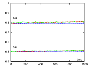
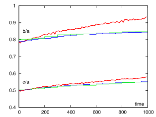
Figure 9: Evolution of the $b/a$ and $c/a$ axial ratios, starting from 0.79 and 0.5, respectively.
The top panel compares two $\gamma=1$ models. The red solid line corresponds to a $N=10^{6}$ reference run, the dotted blue line to a $N=5\cdot 10^{6}$ high-resolution run and the green dash-dotted line to a $N=10^{6}$ model built with the iterative method. They all show little evolution, and the high-resolution run conserves its shape almost perfectly.
The bottom panel shows that the $\gamma=2$, $N_{p}=10^{6}$ simulation (red solid line) shows a substantial evolution of shape. It is compared to the evolutions of orbits in the fixed potential (blue – smooth Dehnen, green – frozen N-body potential), which demonstrate similar amount of shape change exclusively due to chaotic diffusion.

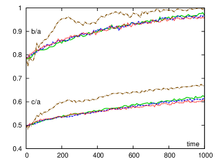
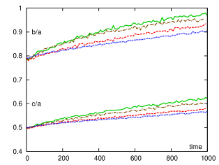
Figure 10: Evolution of the $b/a$ and $c/a$ axial ratios, starting from 0.79 and 0.5, respectively, for variants of the $\gamma=2$ model.
The top panel shows $N_{p}=5\cdot 10^{5}$ particles NM created from SM having $N_{s}=20$ shells and $N_{o}=10^{4}$ orbits integrated for 100 orbital periods. The green solid lines correspond to the unconstrained model, the blue dashed line to the model with a preference of regular orbits, the red dotted line to the model with a preference of chaotic orbits, and the brown dot-dashed to the model created from grid initial conditions (the other three models have random IC). This last one clearly displays the strongest shape evolution, while there is almost no difference between ‘mostly regular’, ‘mostly chaotic’ and ’unconstrained’ models.
The bottom panel shows the effect of particle number in NM and of number of orbits and shells in SM. The green solid line shows the shape evolution of a model with $N_{s}=20,N_{o}=2500$ and $N_{p}=5\cdot 10^{5}$ integrated for 100 dynamical times (same as in the top panel). The brown dot-dashed shows the $N_{s}=50,N_{o}=15000$ and $N_{p}=5\cdot 10^{5}$ model integrated for 100 dynamical times. The red dashed line corresponds to the $N_{s}=50,N_{o}=12500$ and $N_{p}=10^{6}$, integrated for 500 dynamical times (same as the red solid curve in the bottom panel of Fig. 9). The blue dotted line corresponds to a model similar to that of the red line, but with $N_{p}=2\cdot 10^{6}$.
This figure demonstrates that increasing the number of particles does slow down the shape evolution, and that at fixed $N_{p}$ a SM with more shells and orbits behaves better.

For the weak-cusp model (Fig. 9, top panel) the change of axial ratio is very slight for the ‘standard’ model, and virtually zero for high-resolution run with $5\cdot 10^{6}$ particles, which confirms our expectations from the previous section.

In the strong-cusp case (bottom panel), however, the changes are much more obvious. In part, they may be attributed to the much more efficient two-body relaxation in the centre. However, chaotic diffusion may also play a substantial role in this, as demonstrated by integrations in the corresponding fixed potential (Section 4). As seen from the lower panel of Fig. 9, the rate of change of the axial ratio in the fixed-potential integration is comparable to, or, more precisely, about half that of the live N-body model.

6 Exploring the variants of Schwarzschild models

As is well known, Schwarzschild modelling is a rather flexible approach, in the sense that there are many ways to construct models satisfying a given density profile. In fact, the non-uniqueness of the solution may sometimes be an unwanted property of the SM, since there may be no a priori way to tell which one is preferred. Here we explore how the variation of model parameters affects its ‘quality’ and stability. In this section we consider only the $\gamma=2$ case, which displays a more rapid evolution.

The first parameter to vary is the velocity anisotropy. This need not be constant with radius, but the most obvious effect occurs when we change its value at the centre. For $\gamma=1$, the radial-orbit instability is triggered when $\beta$ rises to 0.4, with the axial ratios dropping quickly (withing few time units) from 0.8 to 0.6 ($b/a$) and from 0.5 to 0.4 ($c/a$). This confirms the results of Antonini et al. (2009). For $\gamma=2$, the instability occurs promptly for $\beta=0.5$, with the axis ratios dropping to $b/a=0.5$ and $c/a=0.33$, but it happens, albeit with less dramatic results, even for $\beta$ as small as 0.1, when the ratios instantly drop by a few percent. The subsequent evolution of axis ratios is slow and similar to the case with no short-term instability.

Next, we fix the velocity anisotropy profile to a $\beta$ growing linearly with the shell number from 0 in the centre to 0.6 in the outer parts, so that the model becomes robust against the radial orbit instability, and study the effect of changing the relative fraction of chaotic orbits in the SM. There is still considerable freedom in distributing orbit weights between regular and chaotic orbits. By inserting penalty terms to the objective function that gives preference to regular or to chaotic orbits, a solution may be constructed having a fraction of regular orbits anywhere between 30(35)% and 90(75)% for the $\gamma=1(2)$ cases, respectively, with the ‘unconstrained’ solution yielding $\sim 60\%$ of regular orbits. (These numbers are given for the SM integrated for 100 dynamical times; for $T=500$ models the available range is narrower). The available interval for the fraction of regular orbits is narrower for the strong-cusp case because of the scarcity of stable orbit families in this potential. Most importantly, no solution having only regular orbits may be constructed in both cases.

Other factors to explore include the number of shells $N_{s}$ and of orbits $N_{o}$ in SM, and the ‘coverage’ of the accessible phase space by orbits. The latter factor measures how well and how uniformly an orbit samples its available phase space (invariant 3-dimensional torus for a regular orbit, or a higher-dimension volume of phase space for a chaotic one). As the chaotic orbits sometimes exhibit strong stickiness, it has been proposed to add some noise to the equations of motion to enhance the ‘diffusion rate’ (Kandrup et al., 2000), or – alternatively – to use a ‘dithering method’, proposed in van den Bosch et al. (2008): integrating a bunch of adjacent orbits with slightly perturbed initial conditions and use averaged values of cell occupation times.

In addition, we consider the effects of varying the parameters of NM: number of particles $N_{p}$ and smoothing length $\epsilon$.

The conclusions from these studies are the following. We concentrate mainly on the axis ratio evolution rate (Fig. 10), as it is the most apparent indicator of model instability.

First, all attempts to control the evolution by changing the amount of chaotic orbits in the SM fail miserably – all three models (preferentially regular, chaotic or unconstrained) evolve at the same rate. Secondly, models with more nonzero weight orbits in the SM and/or with more radial shells, tend to perform better, presumably because they are closer to equilibrium and because their distribution function is smoother in phase space. A particularly striking demonstration of the necessity of such smoothing is the very poor behaviour of the model created with the traditional method of assigning initial conditions on a regular grid of points in two start spaces (stationary and principal-plane) at a small number of fixed energy levels.

Moreover, improving the coverage of the phase space available for individual orbits by adding noise, or increasing integration time, or averaging the contribution of a bunch of nearby orbits, also does not seem to help. This conclusion may seem to be in contradiction with the results of Siopis & Kandrup (2000); Kandrup & Siopis (2003), which indicate that adding noise does increase the chaotic diffusion at the stage of SM, which should in principle lead to a more stable NM.

The reason behind this apparent contradiction is probably the following. These methods indeed may improve coverage of phase space for some chaotic orbits, which then become closer to a ‘fully mixed’ ergodic orbit. But since the solution cannot be obtained using only regular and well-mixed chaotic orbits, we still need some chaotic orbits which retain more or less distinct shape and do not fill uniformly their available phase space (in some cases, we need to increase the total number of orbits in SM to get a feasible solution). But nothing prevents such orbits from experiencing the same type of chaotic diffusion in the perturbed NM potential, and since they comprise in total approximately the same fraction of orbits, regardless of the details of construction of SM, the resulting evolution of NM will be more or less the same. This argument also applies in cases where we vary the fraction of chaotic orbits in the SM, because this formal selection criterion will also consider as regular those orbits that did not seem to be sufficiently chaotic, but may readily become so in the NM. It is important to note that all these conclusions are valid also for integration in the fixed potential.

As for the NM parameters, increasing either the number of particles $N_{p}$, or the smoothing length $\epsilon$ does slow down the shape evolution. The latter effect may be attributed to the fact that larger smoothing destroys the strong cusp that is responsible for chaotic diffusion. Therefore, the dynamical properties and phase space structure of such a smoothed model are different from the ones in SM. The increase of particle number does slow down two-body relaxation, but this can not be the main reason for the slow-down of the shape evolution because the timescale for chaotic diffusion is in any case much shorter than the relaxation time (as seen from Fig. 4, the latter is $\sim 20-50$ times longer than the integration time even for $N_{p}=10^{6}$). Instead, it must be the decrease of the potential graininess due to the increase of the particle number that will be responsible for the increase of the chaotic diffusion time-scale. However, there is probably a fundamental lower limit of the rate of chaotic diffusion, established by the fixed-potential integration experiment (which excluded two-body relaxation), and indeed there seems to be much less difference between $10^{6}$ and $2\cdot 10^{6}$ runs than between $5\cdot 10^{5}$ and $10^{6}$.

7 Comparison with the iterative method for constructing equilibrium models

The iterative method for constructing equilibrium models (Rodionov et al., 2009) is designed to create an N-body model in a stable equilibrium, satisfying given constraints, such as specific density profile, shape, and/or kinematical constraints. This is achieved by performing a series of short-time integrations of any initial NM, and adjusting its properties after each iteration to satisfy the constraints. If this process converges to a solution, it will be stationary in the short term, being in dynamic equilibrium and not having fast growing instabilities. Thus it is worthwhile to compare the properties and evolution of models created with these two different methods – the iterative and the Schwarzschild. We consider here the weak-cusp ($\gamma=1$) case, as we were unable to create a sufficiently stable model for $\gamma=2$ using the iterative method.

The model built with the iterative method has $10^{6}$ particles and a velocity anisotropy ranging from 0 in the centre to 0.7 in the outer parts, similar to our Schwarzschild model. As seen from Fig. 4, these two models have very similar energy diffusion rates, which confirms that SM is indeed in good dynamic equilibrium (since the model built with iterative method should be in equilibrium by definition). The rate of shape evolution is approximately the same for these two types of models (Fig. 9), and the orbit population of the model created with the iterative method is similar to that of SM, being roughly 60%/10%/30% for short-, long-axis tubes and other orbits, correspondingly.

Therefore, we may conclude that the iterative and Schwarzschild methods give similar results, despite being conceptually very different. This supports the idea that orbital content and other properties of a model do not depend substantially on the way it was constructed, provided this was adequate, but depend mainly on the intrinsic properties of the potential.

8 Discussion and conclusions

We studied in detail two triaxial Dehnen models, one with cusp slope $\gamma=1$ (weak cusp) and the other with $\gamma=2$ (strong cusp), both constructed with the Schwarzschild method. Our goal was to check the stability of these models by direct N-body simulations (with a number of particles $N_{p}\geq 10^{6}$), and to explore how the chaotic orbits influence the long-term evolution of model shapes.

The $\gamma=1$ model demonstrated a remarkable stability over the simulation timescale ($\sim 50$ half-mass dynamical times), which confirms earlier results of Holley-Bockelman et al. (2001) obtained, however, for a less triaxial model and for a shorter evolution time, and these of Muzzio et al. (2009) for a cuspy ($\gamma\simeq 1$) model with a similar triaxiality and a quite large ($\geq 50\%$) fraction of chaotic orbits.

The $\gamma=2$ model, on the contrary, displayed substantial shape evolution, increasing the axis ratio $b/a$ from 0.8 to $>0.9$ and $c/a$ from 0.5 to $>0.55$ in a simulation time corresponding to $\sim 200$ half-mass crossing times. We attribute this evolution to chaotic diffusion of orbits, which leads to a similar rate of shape change even for integration in a fixed potential (smooth or frozen-N-body).

The difference between these two models may be explained by the different phase space structure of the underlying potential. In the weak-cusp case there are numerous resonant and thin orbit families, and most chaotic orbits are in fact quite sticky. A similar conclusion about the importance of resonances in preventing chaotic diffusion from changing significantly the overall shape of the model was reached by Valluri et al. (2010). On the contrary, in the strong-cusp case the phase space is relatively ‘simple’, with more strongly chaotic orbits which are rounder in shape. This is in good agreement with the results of Merritt & Quinlan (1998), Holley-Bockelman et al. (2002) and Kalapotharakos et al. (2004) who find that the triaxiality is rapidly destroyed in the presence of a large enough central point mass, which has analogous effect to a strong cusp in terms of degree of chaos (Valluri & Merritt, 1998).

However, the very definition of a chaotic orbit is quite problematic for an N-body model: the only available measure, the frequency diffusion rate ($\delta\omega$), is mainly determined by the change of particle energy during the simulation. Almost all particles in the simulation have $\delta\omega>10^{-2}$, and this quantity has no correlation with the $\delta\omega$ for orbits with the same initial conditions in the smooth potential, even though the shape of an orbit is very similar in the two cases. By contrast, in a frozen-N-body potential $\delta\omega$ is typically in the range $10^{-3}$ to $10^{-2}$ for orbits which are regular in the smooth potential, and is caused by graininess of the potential.

An important conclusion that we reached is that constraining the proportion of stars on chaotic or regular orbits in the N-body model is not of much use for increasing the model stability. The first reason comes directly from the impossibility to detect chaos for orbits in the N-body simulation, discussed in the previous paragraph. The second reason is that there is not much freedom in getting fundamentally different orbit population in SM, when we constrain both the density and velocity anisotropy profile and try to change the amount of stars on chaotic orbits. All that happens really is that we may privilege, in the orbit selection, some inherently chaotic orbits which did not demonstrate sufficiently chaotic behaviour during the orbit integration over those that did; however, in the N-body model both kinds of orbits will be slightly different from their counterparts in SM, and will probably have almost equal chance to contribute to chaotic diffusion. Therefore, it makes no sense to reduce the fraction of chaotic orbits in SM in an attempt to improve the quality (stability) of NM; this is determined mainly by the orbital structure of the underlying potential, and to some degree by a careful construction of SM. We found that increasing the number of orbits in SM does help to reduce evolution, and that randomly assigned initial conditions in SM produce a better model than the conventional method of drawing them from regular grid of points on fixed energy levels.

The arguments about the impossibility of distinguishing between regular and (weakly) chaotic orbits and controlling the nature of any particular orbit in N-body simulation may, at first sight, seem to be grounded on the limited resolution of the simulation and inaccuracies introduced by energy relaxation. However, while the two-body relaxation times in real galaxies are many orders of magnitude longer than in our runs, there are always some large-scale processes that both shuffle stars across phase space and change properties of this phase space, at least to some degree. As such we can mention encounters of stars with globular clusters, or with molecular clouds or with transient spiral segments, which will perturb their trajectories as much as, if not more than they would be by the lower number of bodies in our idealized N-body simulations. Therefore, it is unrealistic to expect that a carefully arranged initial composition of stars mostly on regular orbits will be preserved over a Hubble time. Rather, an unconstrained (in terms of fraction of chaotic orbits) arrangement of orbits, evolving according to the gross properties of the underlying potential, should give a better idea of the typical rate of shape change.

The difference in the evolution of weak- and strong-cusp models – the latter becoming noticeably rounder during the Hubble time – is also in agreement with observations that show that fainter elliptical galaxies which are, on average, more cuspy, have more spherical shapes than brighter ones, which have shallower density profiles and are more triaxial (e.g. Tremblay & Merritt, 1996, and references therein).

Apart from the cases when radial-orbit instability occurs, and from the cases displaying secular shape evolution due to chaotic diffusion, models built with the Schwarzschild method appear to be in stable equilibrium.

Acknowledgments: We are grateful to S. Rodionov for preparing the model built with the iterative method, to F. Antonini and D. Merritt for fruitful discussions, and to the referee for helpful remarks. EV was partially supported by Russian Ministry of science and education (grants No.2009-1.1-126-056 and P1336), and by the CNRS during his visit to the Laboratoire d’Astrophysique de Marseille (UMR6110).

References

- Antonini et al. (2009) Antonini F., Capuzzo-Dolcetta R., Merritt D., 2009, MNRAS, 399, 671
- Aquilano et al. (2007) Aquilano R., Muzzio J., Navone H., Zorzi A., 2007, CeMDA, 99, 307
- Athanassoula & Misiriotis (2002) Athanassoula E., Misiriotis A., 2002, MNRAS, 330, 35
- Binney & Tremaine (2007) Binney J., Tremaine S., 2007, Galactic dynamics, Princeton Univ. Press, Princeton, NJ
- Capuzzo-Dolcetta et al. (2007) Capuzzo-Dolcetta R., Leccese L., Merritt D., Vicari A., 2007, 666, 165
- Contopoulos (1971) Contopoulos G., 1971, AJ, 76, 147
- Contopoulos (2002) Contopoulos G., 2002, Order and chaos in dynamical astronomy, Springer, Berlin
- Dehnen (1993) Dehnen W., 1993, MNRAS, 265, 250
- Dehnen (2000) Dehnen W., 2000, ApJ, 536, L39
- Dehnen (2002) Dehnen W., 2002, J.Comp.phys., 179, 27
- Dubinski & Carlberg (1991) Dubinski J., Carlberg R.., 1991, ApJ, 378, 496
- Hernquist (1990) Hernquist L., 1990, ApJ, 356, 259
- Harsoula & Kalapotharakos (2009) Harsoula M., Kalapotharakos, K., 2009, MNRAS, 394, 1605
- Holley-Bockelman et al. (2001) Holley-Bockelmann K., Mihos J.C., Sigurdsson S., Hernquist L., 2001, ApJ, 549, 862
- Holley-Bockelman et al. (2002) Holley-Bockelmann K., Mihos J.C., Sigurdsson S., Hernquist L., Norman C., 2002, ApJ, 567, 817
- Kalapotharakos et al. (2004) Kalapotharakos C., Voglis N., Contopoulos G., 2004, A&A, 428, 905
- Kandrup et al. (1997) Kandrup H., Eckstein B., Bradley B., 1997, A&A, 320, 65
- Kandrup et al. (2000) Kandrup H., Pogorelov I., Sideris I., 2000, MNRAS, 311, 719
- Kandrup & Sideris (2001) Kandrup H., Sideris I., 2001, Phys.Rev.E, 64, 056209
- Kandrup & Sideris (2003) Kandrup H., Sideris I., 2003, ApJ, 585, 244
- Kandrup & Siopis (2003) Kandrup H., Siopis C., 2003, MNRAS, 345, 727
- Laskar (1993) Laskar J., 1993, Physica D, 67, 257
- Merritt & Fridman (1996) Merritt D., Fridman T., 1996, ApJ, 460, 136
- Merritt & Quinlan (1998) Merritt D., Quinlan G., 1998, ApJ, 498, 625
- Merritt & Valluri (1996) Merritt D., Valluri M., 1996, ApJ, 471, 82
- Muzzio et al. (2005) Muzzio J., Carpintero D., Wachlin F., 2005, CeMDA, 91, 173
- Muzzio et al. (2009) Muzzio J., Navone H., Zorzi A., 2009, CeMDA, 105, 379
- Pfenniger (1984) Pfenniger D., 1984, A&A, 141, 171
- Polyachenko & Schukhman (1981) Polyachenko V.L., Shukhman I.G., 1981, Sov.Ast., 25, 533
- Poon & Merritt (2004) Poon M.-Y., Merritt D., 2004, ApJ, 606, 774
- Rodionov et al. (2009) Rodionov S.A., Athanassoula E., Sotnikova N.Ya., 2009, MNRAS, 392, 904
- Schwarzschild (1979) Schwarzschild M., 1979, ApJ, 232, 236
- Schwarzschild (1993) Schwarzschild M., 1993, ApJ, 409, 563
- Sideris & Kandrup (2002) Sideris I., Kandrup H., 2002, Phys.Rev.E, 65, 066203
- Siopis (1999) Siopis C., 1999, PhD thesis, Univ. Florida
- Siopis & Kandrup (2000) Siopis C., Kandrup H., 2000, MNRAS, 319, 43
- Skokos (2010) Skokos Ch., 2010, in Souchay J. and Dvorak R., eds, Dynamics of Small Solar System Bodies and Exoplanets, Lecture Notes in Physics Vol. 790 Springer Berlin / Heidelberg, p.63
- Smith & Miller (1982) Smith B F, Miller R.H., 1982, ApJ, 257, 103
- Terzić (2002) Terzić B., 2002, PhD thesis, Univ. Florida
- Tremblay & Merritt (1996) Tremblay B., Merritt D., 1996, AJ, 111, 2243
- Valluri & Merritt (1998) Valluri M., Merritt D., 1998, ApJ, 506, 686
- Valluri & Merritt (2000) Valluri M., Merritt D., 2000, in Gurzadyan V.G., Ruffini R., eds, The Chaotic Universe, World Scientific, Advanced Series in Astrophysics and Cosmology, 10, p.229
- Valluri et al. (2010) Valluri M., Debattista V., Quinn T., Moore B., 2010, MNRAS, 403, 525
- van den Bosch et al. (2008) van den Bosch R.C.E., van de Ven G., Verolme E.K., Cappellari M., de Zeeuw P.T., 2008, MNRAS, 385, 647
- Wu et al. (2009) Wu X., Zhao H.-S., Wang Y., Llinares C., Knebe A., 2009, MNRAS, 396, 109
- Zemp et al. (2011) Zemp M., Gnedin O., Gnedin N., Kravtsov A., 2011, arXiv:1107.5582
- Zhao (1996) Zhao H.-S., 1996, MNRAS, 283, 149