HAT-P-34b — HAT-P-37b: Four Transiting Planets More Massive Than Jupiter Orbiting Moderately Bright Stars

Abstract

We report the discovery of four transiting extrasolar planets (HAT-P-34b–HAT-P-37b) with masses ranging from $1.05$ to $3.33$ $M_{\rm J}$ and periods from 1.33 to 5.45 days. These planets orbit relatively bright F and G dwarf stars (from $V=10.16$ to $V=13.2$). Of particular interest is HAT-P-34b which is moderately massive ($3.33$ $M_{\rm J}$), has a high eccentricity of $e=0.441\pm 0.032$ at $P=5.452654\pm 0.000016\,d$ period, and shows hints of an outer component. The other three planets have properties that are typical of hot Jupiters.

1. Introduction

Transiting extrasolar planets (TEPs) provide unique opportunities to study the properties of planetary objects outside of the Solar System. To date well over 100 such planets have been discovered and characterized, leading to numerous insights into the physical properties of planetary systems (e.g. see the recent review by Rauer, 2011). In addition, over a thousand strong candidates from Kepler have been identified (Borucki et al., 2011), greatly expanding our understanding of several aspects of planetary systems, such as the properties of multi-planet systems (Latham et al., 2011; Lissauer et al., 2011), and the distribution of planetary radii (Howard et al., 2011). However, due to the large number of important variables which influence the physical properties of a planet (e.g. its mass, composition, age, irradiation, and tides, to name a few), we are still far from an empirically tested, comprehensive understanding of the formation and evolution of planetary systems.

Here we present the discovery of four new TEPs identified by the Hungarian-made Automated Telescope Network (HATNet; Bakos et al., 2004) survey which contribute to the rapidly-growing sample of TEPs. These planets transit relatively bright stars facilitating detailed characterization of their properties, such as measurements of their masses via radial velocity (RV) observations of the host star, or measuring their orbital tilt via the Rossiter-McLaughlin effect.

The HATNet survey for TEPs around bright stars ($9\lesssim r\lesssim 14.5$) operates six wide-field instruments: four at the Fred Lawrence Whipple Observatory (FLWO) in Arizona (HAT-5, -6, -7, and -10), and two on the roof of the hangar servicing the Smithsonian Astrophysical Observatory’s Submillimeter Array, in Hawaii (HAT-8 and -9). Since 2006, HATNet has announced and published 33 TEPs (e.g. Johnson et al., 2011). In this work we report our thirty-fourth through thirty-seventh discoveries, around the stars GSC 1622-01261, GSC 0203-01079, GSC 3020-02221, and GSC 3553-00723.

In Section 2 we summarize the detection of the photometric transit signals and the subsequent spectroscopic and photometric observations of each star to confirm the planets. In Section 3 we analyze the data to determine the stellar and planetary parameters. The properties of these planets are briefly discussed in Section 4.

Table 1 Summary of discovery data.

Planet Host	GSC	2MASS	RA	DEC	V	Depth	Period
			HH:MM:SS	DD:MM:SS	mag	mmag	days
HAT-P-34	1622-01261	20124688+1806175	$20^{\mathrm{h}}12^{\mathrm{m}}46.80{\mathrm{s}}$	$+18{\arcdeg}06{\arcmin}17.5{\arcsec}$	$10.162\pm 0.073$	$7.9$	$5.4527$
HAT-P-35	0203-01079	08130018+0447132	$08^{\mathrm{h}}13^{\mathrm{m}}00.19{\mathrm{s}}$	$+04{\arcdeg}47{\arcmin}13.3{\arcsec}$	$12.46\pm 0.11$	$9.0$	$3.6467$
HAT-P-36	3020-02221	12330390+4454552	$12^{\mathrm{h}}33^{\mathrm{m}}03.96{\mathrm{s}}$	$+44{\arcdeg}54{\arcmin}55.3{\arcsec}$	$12.262\pm 0.068$	$14.7$	$1.3273$
HAT-P-37	3553-00723	18571105+5116088	$18^{\mathrm{h}}57^{\mathrm{m}}11.16{\mathrm{s}}$	$+51{\arcdeg}16{\arcmin}08.9{\arcsec}$	$13.23\pm 0.32$	$18.1$	$2.7974$

2. Observations

The observational procedure employed by HATNet to discover TEPs has been described in detail in several previous discovery papers (e.g. Bakos et al., 2010; Latham et al., 2009). In the following subsections we highlight specific details of this procedure that are pertinent to the discoveries of the four planets presented in this paper.

2.1. Photometric detection

Table 2 summarizes the HATNet discovery observations of each new planetary system. The HATNet images were processed and reduced to trend-filtered light curves following the procedure described by Bakos et al. (2010) and Pál (2009b). The light curves were searched for periodic box-shaped signals using the Box Least-Squares (BLS; see Kovács et al., 2002) method. We detected significant signals in the light curves of the stars summarized in Table 1.

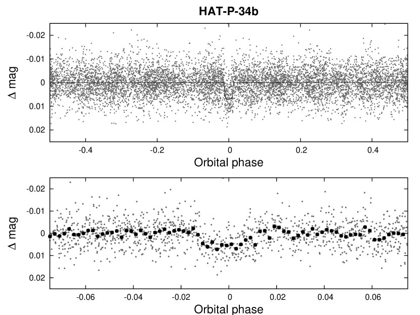
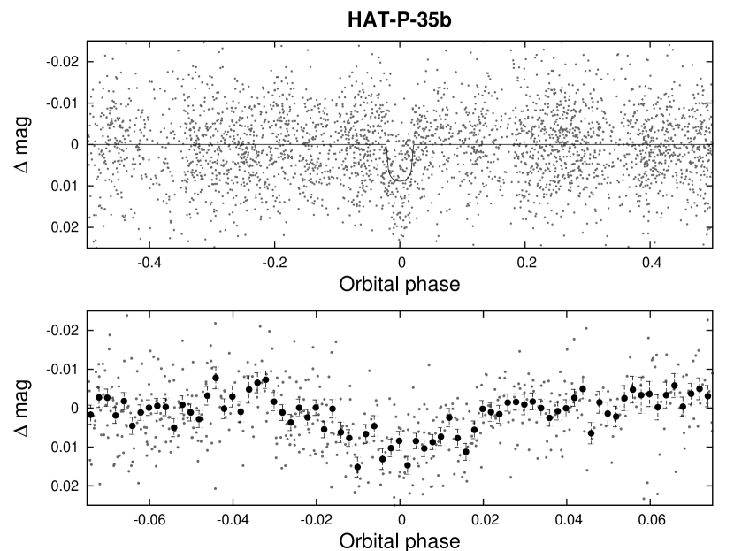
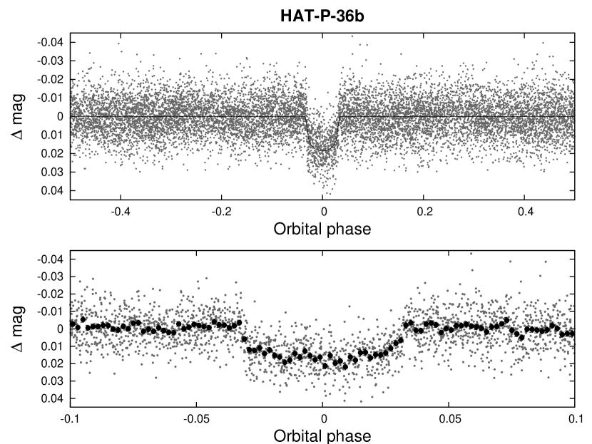
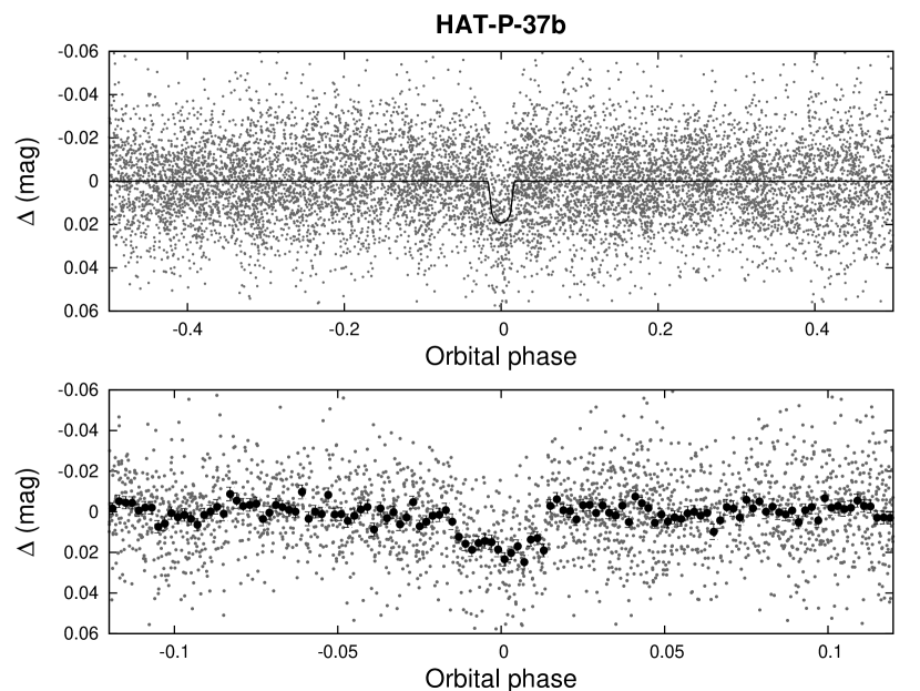
Figure 1.— HATNet light curves of HAT-P-34 through HAT-P-37. See Table 2 for a summary of the observations. For each planet we show two panels. The top panel shows the unbinned light curve folded with the period resulting from the global fit described in Section 3. The solid line shows the model fit to the light curve (Section 3.2). The bottom panel shows the region zoomed-in on the transit. The dark filled circles show the light curve binned in phase with a binsize of 0.002.

Table 2 Summary of photometric observations

Instrument/Field	Date(s)	Number of Images	Cadence (sec)	Filter
HAT-P-34
HAT-7/G293	2008 Oct–2009 May	755	$330$	$r$
HAT-8/G293	2008 Sep–2008 Dec	2611	$330$	$r$
HAT-6/G341	2007 Sep–2007 Dec	1949	$330$	$R$
HAT-9/G341	2007 Sep–2007 Nov	2379	$330$	$R$
KeplerCam	2010 May 21	263	$60$	$z$
KeplerCam	2010 Oct 10	530	$30$	$i$
HAT-P-35
HAT-5/G364	2009 May	21	$330$	$r$
HAT-9/G364	2008 Dec–2009 May	3155	$330$	$r$
KeplerCam	2011 Jan 16	110	$100$	$i$
FTN	2011 Jan 23	185	$45$	$i$
KeplerCam	2011 Mar 08	268	$60$	$i$
HAT-P-36
HAT-5/G143	2010 Apr–2010 Jul	4471	$210$	$r$
HAT-8/G143	2010 Apr–2010 Jul	6262	$210$	$r$
KeplerCam	2010 Dec 24	131	$130$	$i$
KeplerCam	2011 Feb 03	101	$100$	$i$
KeplerCam	2011 Feb 07	105	$100$	$i$
KeplerCam	2011 Feb 15	186	$60$	$i$
HAT-P-37
HAT-7/G115	2009 Sep–2010 Jul	7102	$210$	$r$
HAT-9/G115	2008 Aug–2008 Sep	2293	$330$	$R$
KeplerCam	2011 Feb 23	37	$165$	$i$
KeplerCam	2011 Mar 23	73	$134$	$i$
KeplerCam	2011 Apr 06	102	$134$	$i$

2.2. Reconnaissance Spectroscopy

High-resolution, low-S/N “reconnaissance” spectra were obtained for HAT-P-34 and HAT-P-35 using the Tillinghast Reflector Echelle Spectrograph (TRES; Fűrész, 2008) on the 1.5 m Tillinghast Reflector at FLWO. These observations were reduced and analyzed following the procedure described by Quinn et al. (2010) and Buchhave et al. (2010); the results are listed in Table 3. For both objects the spectra were single-lined, and showed radial velocity (RV) variations on the order of $\sim 100$ $\rm m\,s^{-1}$. Proper phasing of the RV with the photometric ephemeris gives confidence in acquiring further, high signal-to-noise spectroscopic observations to refine the orbit (see § 2.3). While for HAT-P-34 the variations initially did not appear to phase with the photometric ephemeris, we entertained the possibility of a very significant non-zero eccentricity, and pursued follow-up of the target. For HAT-P-35 the variations were in phase with the photometric ephemeris indicating a $\sim 2.7\,M_{\rm J}$ companion. For both HAT-P-36 and HAT-P-37 we obtained two TRES spectra near each of the predicted quadrature phases. For both objects the spectra were single-lined. For HAT-P-36 the resulting RV measurements showed $\sim 400$ $\rm m\,s^{-1}$ variation in phase with the photometric ephemeris, while for HAT-P-37 the RV measurements showed $\sim 260$ $\rm m\,s^{-1}$ variation in phase with the ephemeris. We opted to continue observing both of these objects using TRES with the aim of confirming the planets. The TRES observations of HAT-P-36 and HAT-P-37 are discussed further in the following subsection.

Table 3 Summary of reconnaissance spectroscopy observations

Instrument	HJD	$\gamma_{\rm RV}$	CC Peak
		($\rm km\,s^{-1}$)
HAT-P-34
TRES	$2454935.00839$	$-47.81$	$0.726$
TRES	$2454966.97204$	$-49.19$	$0.939$
TRES	$2454998.97956$	$-49.12$	$0.819$
HAT-P-35
TRES	$2455289.64284$	$41.24$	$0.863$
TRES	$2455291.62482$	$40.54$	$0.883$
TRES	$2455320.64182$	$40.83$	$0.935$
TRES	$2455321.64383$	$41.08$	$0.940$

2.3. High resolution, high S/N spectroscopy

We proceeded with the follow-up of each candidate by obtaining high-resolution, high-S/N spectra to characterize the RV variations, and to refine the determination of the stellar parameters. These observations are summarized in Table 4. The RV measurements and uncertainties for HAT-P-34 through HAT-P-37 are given in the Appendix, and in Tables A–A, respectively. The period-folded data, along with our best fit described below in Section 3, are displayed in Figures 2–5.

Four facilities were used in the confirmation of these planets (including three separate facilities used for HAT-P-34). These facilities are HIRES (Vogt et al., 1994) on the 10 m Keck I telescope in Hawaii, the High-Dispersion Spectrograph (HDS; Noguchi et al., 2002) on the 8.3 m Subaru telescope in Hawaii, the FIbre-fed Échelle Spectrograph (FIES) on the 2.5 m Nordic Optical Telescope (NOT) at La Palma, Spain (Djupvik & Andersen, 2010), and TRES on the FLWO 1.5 m telescope.

The HIRES and HDS observations made use of the iodine-cell method (Marcy & Butler, 1992; Butler et al., 1996) for precise wavelength calibration and relative RV determination, while the FIES and TRES observations made use of Th-Ar lamp spectra obtained before and after the science exposures. The HIRES observations were reduced to relative RVs in the barycentric frame following Butler et al. (1996), Johnson et al. (2009), and Howard et al. (2010), the HDS observations were reduced following Sato et al. (2002, 2005), and the FIES and TRES observations were reduced following Buchhave et al. (2010).

We found that for all four systems the RV residuals from the best-fit models, described below in Section 3.2, exhibit excess scatter over what is expected based on the formal measurement uncertainties. Such excess scatter, or “jitter” has been well known for stars, and can stem for multiple sources. The excess is in the residuals of the observations with respect to a physical (and possibly instrumental) model. If this model is not adequate, the residuals can be larger than expected. For example, in the case of HAT-P-34b, ignoring the linear trend in the RVs would lead to a much increased “jitter”. Additional planets may cause jitter, as the limited number of RV observations is not enough to uniquely identify and model such systems. The typical source of the jitter, however, is the star itself, namely inhomogeneities (spots, flares, plages, etc.) on the stellar surface (e.g. Makarov et al., 2009; Martínez-Arnáiz et al., 2010) causing jitters up to 100 ms. Granulation and stellar oscillations contribute at a smaller scale, but are present for non-active stars that are outside the instability strip. A recent publication by Cegla et al. (2012) discusses the stellar jitter due to variable gravitational redshift of the star, as the stellar radius changes due to oscillations ($\Delta R$ of $10^{-4}$ causing $\sim 0.1\,\rm m\,s^{-1}$). And, of course, systematics in the instrument further inflate the jitter. A review of RV jitter of stars observed by the Keck telescope are given in Wright (2005).

In order to ensure realistic estimates of the system parameter uncertainties we add in quadrature an RV jitter to the formal RV measurement uncertainties such that $\chi^{2}$ per degree of freedom is unity for the best-fit model for each planet. We adopt an independent jitter for the observations made by each instrument of each planet. The RV uncertainties given in Tables A–A do not include this jitter; we do include the jitter in Figures 2–5.

Table 4 Summary of high-SN spectroscopic observations used in measuring the orbits

Instrument	Date(s)	Number of
		RV obs.
HAT-P-34
Subaru/HDS	2010 May	6
Keck/HIRES	2010 Jun–2010 Sep	14
NOT/FIES	2010 Jul–2010 Aug	10
HAT-P-35
Keck/HIRES	2010 Sep–2010 Dec	7
NOT/FIES	2010 Oct	5
HAT-P-36
FLWO 1.5/TRES	2010 Dec–2011 Jan	12
HAT-P-37
FLWO 1.5/TRES	2011 Mar–2011 May	13

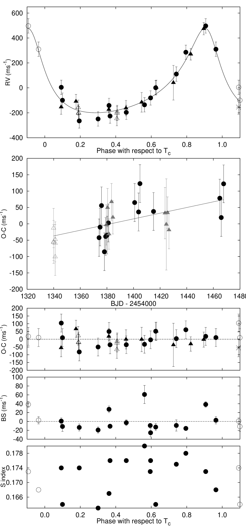
Figure 2.— Top panel: High-precision RV measurements for HAT-P-34 shown as a function of orbital phase, along with our best-fit model (see Table 6). Open triangles show measurements from Subaru/HDS, filled circles show measurements from Keck/HIRES, and filled triangles show measurements from NOT/FIES. Zero phase corresponds to the time of mid-transit. The center-of-mass velocity and a linear trend have been subtracted. Second panel: velocity $O\!-\!C$ residuals from the best-fit single Keplerian orbit model as a function of time. The residuals show a slight linear trend, possibly indicating a third body in the system. Note that the zero-points of the three separate instruments are independently free parameters. Third panel: velocity $O\!-\!C$ residuals from the best fit including both the Keplerian orbit and linear trend, shown as a function of orbital phase. The error bars include a jitter term ($56.0$ $\rm m\,s^{-1}$ for the Keck/HIRES observations, and $32.0$ $\rm m\,s^{-1}$ for the Subaru/HDS observations; no jitter has been added to the NOT/FIES RV uncertainties) added in quadrature to the formal errors (see Section 3.2). Fourth panel: bisector spans (BS) from Keck/HIRES, with the mean value subtracted. The measurement from the template spectrum is included. Bottom panel: Chromospheric activity index $S$ measured from the Keck spectra. Note the different vertical scales of the panels. Observations shown twice are represented with open symbols.

Figure 3.— Keck/HIRES observations of HAT-P-35. The panels are as in Figure 2. The parameters used in the best-fit model are given in Table 6.

Figure 4.— FLWO 1.5 m/TRES observations of HAT-P-36. The panels are as in Figure 2. The $S$ index is not available for these observations. The parameters used in the best-fit model are given in Table 6.

Figure 5.— FLWO 1.5 m/TRES observations of HAT-P-37. The panels are as in Figure 2. The $S$ index is not available for these observations. The parameters used in the best-fit model are given in Table 6.

For HAT-P-34 and HAT-P-35 we also show the $S$ index, which is a measure of the chromospheric activity of the star derived from the flux in the cores of the Ca II H and K lines. This index was computed following Isaacson & Fischer (2010) and has been calibrated to the scale of Vaughan, Preston & Wilson (1978). A procedure for obtaining calibrated $S$ index values from the TRES spectra has not yet been developed, so we do not provide these measurements for HAT-P-36 or HAT-P-37. We convert the $S$ index values to $\log R^{\prime}_{\rm HK}$ following Noyes et al. (1984) and find median values of $\log R^{\prime}_{\rm HK}=-4.859$ and $\log R^{\prime}_{\rm HK}=-5.242$ for HAT-P-34 and HAT-P-35, respectively. These values imply that neither star has a particularly high level of chromospheric activity.

Following Queloz et al. (2001) and Torres et al. (2007), we checked whether the measured radial velocities are not real, but are instead caused by distortions in the spectral line profiles due to contamination from a nearby unresolved eclipsing binary. A bisector (BS) analysis for each system based on the Keck and TRES spectra was done as described in §5 of Bakos et al. (2007a). For HAT-P-35, which is relatively faint, we found that the measured BSs were significantly affected by scattered moonlight and applied an empirical correction for this effect following Hartman et al. (2009) (see also Kovács et al. (2010)). For HAT-P-34 the BS scatter is fairly high ($\sim 25$ $\rm m\,s^{-1}$), but this is in line with the high RV jitter ($\sim 60$ $\rm m\,s^{-1}$), which is typical of an F star with $v\sin{i}=24.0\pm 0.5$ $\rm km\,s^{-1}$ (Saar et al., 2003; Hartman et al., 2011b).

None of the systems show significant bisector span variations (relative to the semi-amplitude of the RV variations) that phase with the photometric ephemeris. Such variations are generally expected if the transit and RV signals were due to blends rather than planets. While the lack of bisector span variations does not exclude all blend scenarios, it does significantly limit the possible blend scenarios that can reproduce our current data within the measurement errors, i.e. configurations that are compatible with the photometric and spectroscopic observations, proper motions, color indices, and moderately high resolution imaging. We have found in the past that invoking detailed blend modeling to exclude all possible blend configurations and confirm the planet hypothesis (e.g. Hartman et al., 2011a, sections 3.2.2, 3.2.3) is rarely of any incremental value when the ingress and egress durations are short relative to the total transit duration, the RV variations exhibit a Keplerian orbit in phase with the photometric ephemeris, and bisector spans show no correlation with the orbit. We conclude that the velocity variations detected for all four stars are real, and that each star is orbited by a close-in giant planet.

2.4. Photometric follow-up observations

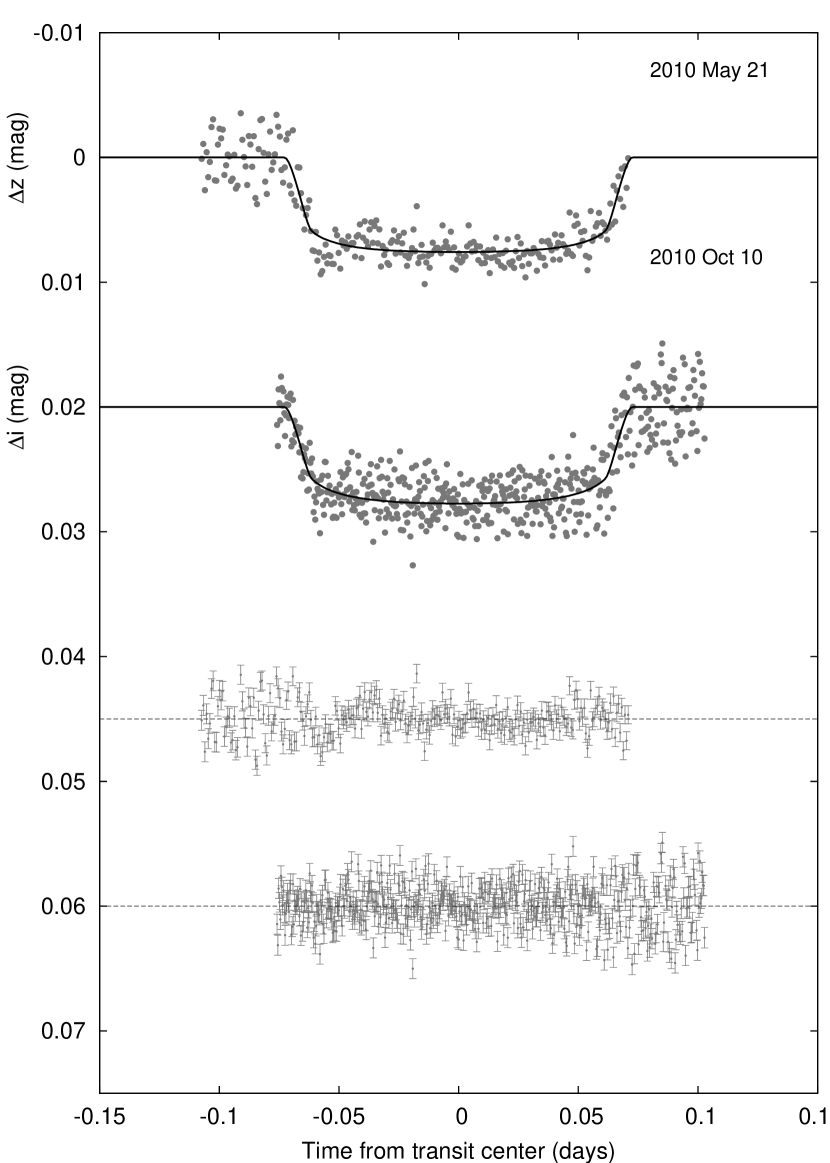
Figure 6.— Unbinned transit light curves for HAT-P-34, acquired with KeplerCam at the FLWO 1.2 m telescope. The light curves have been EPD- and TFA-processed, as described in § 3.2. The dates of the events are indicated. Curves after the first are displaced vertically for clarity. Our best fit from the global modeling described in Section 3.2 is shown by the solid lines. Residuals from the fits are displayed at the bottom, in the same order as the top curves. The error bars represent the photon and background shot noise, plus the readout noise.

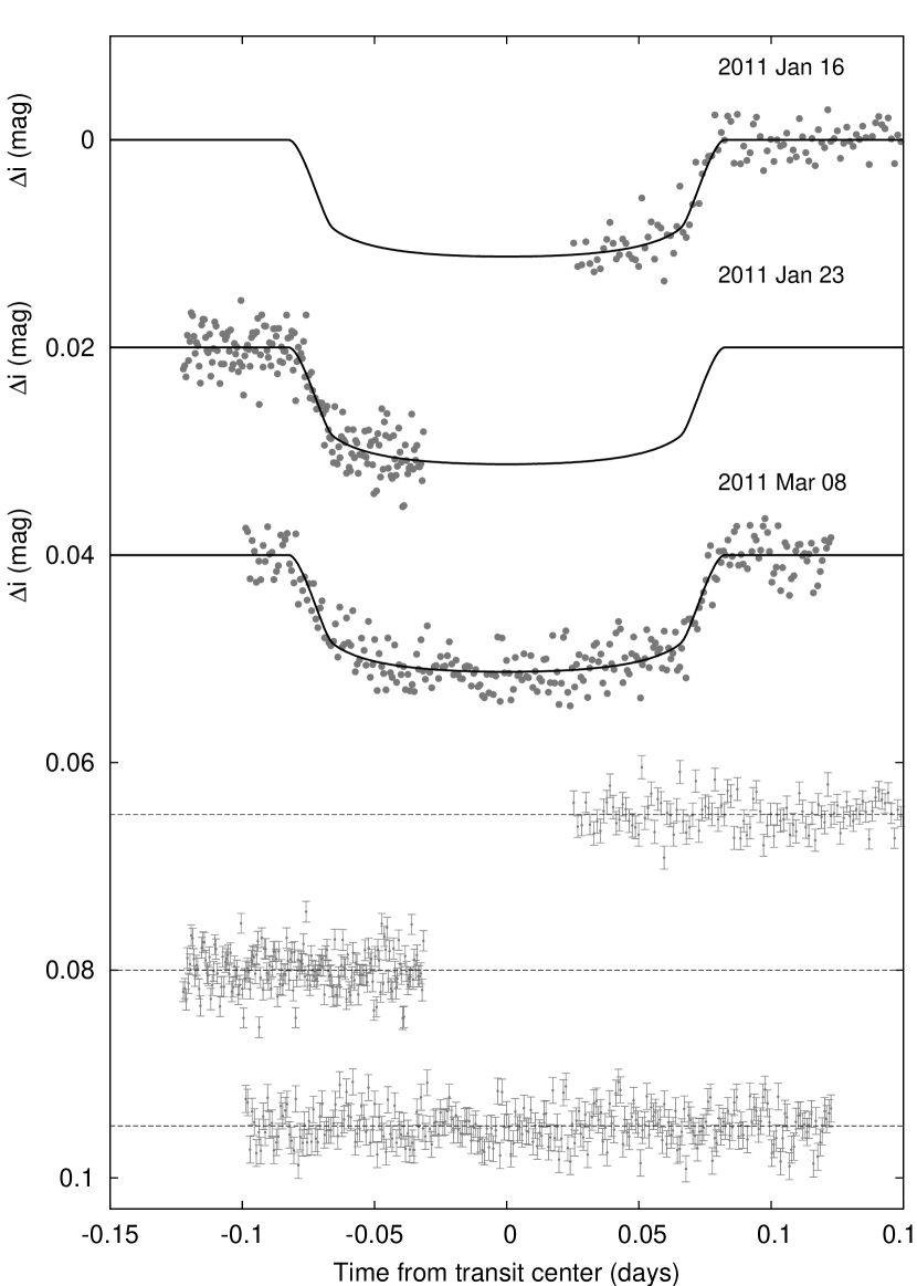
Figure 7.— Similar to Figure 6; here we show the follow-up light curves for HAT-P-35.

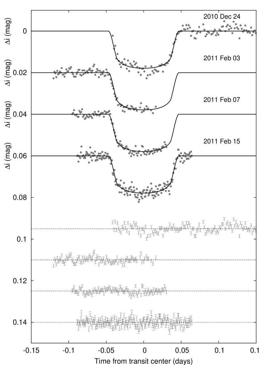
Figure 8.— Similar to Figure 6; here we show the follow-up light curves for HAT-P-36.

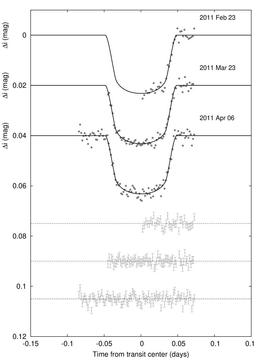
Figure 9.— Similar to Figure 6; here we show the follow-up light curves for HAT-P-37.

In order to permit a more accurate modeling of the light curves, we conducted additional photometric observations using the KeplerCam CCD camera on the FLWO 1.2 m telescope, and the Spectral Instrument CCD on the 2.0 m Faulkes Telescope North (FTN) at Haleakala Observatory in Hawaii, which is operated by the Las Cumbres Observatory Global Telescope (LCOGT). The observations for each target are summarized in Table 2.

The reduction of these images was performed as described by Bakos et al. (2010). We applied External Parameter Decorrelation (EPD; Bakos et al., 2010) and the Trend Filtering Algorithm (TFA; Kovács et al., 2005) to remove trends simultaneously with the light curve modeling. The final time series, together with our best-fit transit light curve models, are shown in the top portion of Figures 6–9 for HAT-P-34 through HAT-P-37, respectively. The individual measurements, permitting independent analysis by other researchers, are reported in the Appendix, in Tables A–A (the full data are available in electronic format).

3. Analysis

Figure 10.— Comparison of the measured values of $T_{\rm eff\star}$ and $a/R_{\star}$ for HAT-P-34 (upper left), HAT-P-35 (upper right), HAT-P-36 (lower left) and HAT-P-37 (lower right) to model isochrones from Yi et al. (2001). The isochrones are generated for the measured metallicity of each star, and for ages of 0.5 Gyr and 1 to 3 Gyr in steps of 0.25 Gyr for HAT-P-34, and of 0.5 Gyr and 1 to 14 Gyr in steps of 1 Gyr for HAT-P-35, HAT-P-36 and HAT-P-37 (ages increase from left to right in each plot). The lines show the 1$\sigma$ and 2$\sigma$ confidence ellipses for the measured parameters. The initial values of $T_{\rm eff\star}$ and $a/R_{\star}$ from the initial spectroscopic and light curve analyses are represented with a triangle in each panel.

3.1. Properties of the parent star

Table 5 Stellar parameters for HAT-P-34 through HAT-P-37

	HAT-P-34	HAT-P-35	HAT-P-36	HAT-P-37
Parameter	Value	Value	Value	Value	Source
Spectroscopic properties
$T_{\rm eff\star}$ (K)	$6442\pm 88$	$6096\pm 88$	$5560\pm 100$	$5500\pm 100$	Spec. Analysis.
$\rm[Fe/H]$	$+0.22\pm 0.04$	$+0.11\pm 0.08$	$+0.26\pm 0.10$	$+0.03\pm 0.10$	Spec. Analysis.
$v\sin{i}$ ($\rm km\,s^{-1}$)	$24.0\pm 0.5$	$0.5\pm 0.5$	$3.58\pm 0.5$	$3.07\pm 0.5$	Spec. Analysis.
$v_{\rm mac}$ ($\rm km\,s^{-1}$)	$5.05$	$4.52$	$0.00$	$\ldots$	Spec. Analysis.
$v_{\rm mic}$ ($\rm km\,s^{-1}$)	$0.85$	$0.85$	$0.00$	$\ldots$	Spec. Analysis.
$\gamma_{\rm RV}$ ($\rm km\,s^{-1}$)	$-49.26\pm 0.30$	$40.95\pm 0.20$	$-16.29\pm 0.10$	$-20.53\pm 0.1$	TRES
Photometric properties
$V$ (mag)	$10.162\pm 0.073$	$12.46\pm 0.11$	$12.262\pm 0.068$	$13.23\pm 0.32$	TASS,GSC
$V\!-\!I_{C}$ (mag)	$0.557\pm 0.12$	$0.662\pm 0.12$	$0.760\pm 0.13$	$\cdots$	TASS
$J$ (mag)	$9.460\pm 0.022$	$11.358\pm 0.024$	$11.046\pm 0.027$	$12.092\pm 0.027$	2MASS
$H$ (mag)	$9.322\pm 0.030$	$11.072\pm 0.023$	$10.723\pm 0.030$	$11.714\pm 0.032$	2MASS
$K_{s}$ (mag)	$9.247\pm 0.023$	$11.030\pm 0.021$	$10.603\pm 0.021$	$11.667\pm 0.020$	2MASS
Derived properties
$M_{\star}$ ($M_{\sun}$)	$1.392\pm 0.047$	$1.236\pm 0.048$	$1.022\pm 0.049$	$0.929\pm 0.043$	YY+$a/R_{\star}$+Spec. Analysis.
$R_{\star}$ ($R_{\sun}$)	$1.535_{-0.102}^{+0.135}$	$1.435\pm 0.084$	$1.096\pm 0.056$	$0.877_{-0.044}^{+0.059}$	YY+$a/R_{\star}$+Spec. Analysis
$\log{g_{\star}}$ (cgs)	$4.21\pm 0.06$	$4.21\pm 0.04$	$4.37\pm 0.04$	$4.52\pm 0.05$	YY+$a/R_{\star}$+Spec. Analysis
$L_{\star}$ ($L_{\sun}$)	$3.63_{-0.51}^{+0.75}$	$2.55_{-0.30}^{+0.40}$	$1.03\pm 0.15$	$0.62_{-0.09}^{+0.11}$	YY+$a/R_{\star}$+Spec. Analysis
$M_{V}$ (mag)	$3.32\pm 0.19$	$3.77\pm 0.15$	$4.83\pm 0.17$	$5.41\pm 0.19$	YY+$a/R_{\star}$+Spec. Analysis
$M_{K}$ (mag,ESO)	$2.24\pm 0.17$	$2.43\pm 0.13$	$3.14\pm 0.12$	$3.64\pm 0.14$	YY+$a/R_{\star}$+Spec. Analysis
Age (Gyr)	$1.7_{-0.5}^{+0.4}$	$3.5_{-0.5}^{+0.8}$	$6.6_{-1.8}^{+2.9}$	$3.6_{-2.2}^{+4.1}$	YY+$a/R_{\star}$+Spec. Analysis
Distance (pc)	$257_{-17}^{+22}$0	$535\pm 32$0	$317\pm 17$0	$411\pm 26$0	YY+$a/R_{\star}$+Spec. Analysis

Stellar atmospheric parameters for HAT-P-34 and HAT-P-35 were measured using our template spectra obtained with the Keck/HIRES instrument, and the analysis package known as Spectroscopy Made Easy (SME; Valenti & Piskunov, 1996), along with the atomic line database of Valenti & Fischer (2005). For HAT-P-36 and HAT-P-37 the stellar atmospheric parameters were determined by cross-correlating the TRES observations against a finely sampled grid of synthetic spectra based on Kurucz (2005) model atmospheres. This procedure, known as Stellar Parameter Classification (SPC), will be described in detail in a forthcoming paper (Buchhave et al., in preparation). We note that SPC has been performed in the past on numerous HATNet transiting planet candidates (Buchhave, personal communication), and the results were consistent with those of SME.

For each star, we obtained the following initial spectroscopic parameters and uncertainties:

• HAT-P-34 – effective temperature $T_{\rm eff\star}=6400\pm 100$ K, metallicity $\rm[Fe/H]=+0.21\pm 0.1$ dex, stellar surface gravity $\log{g_{\star}}=3.98\pm 0.1$ (cgs), and projected rotational velocity $v\sin{i}=24.5\pm 1.0$ $\rm km\,s^{-1}$.

• HAT-P-35 – effective temperature $T_{\rm eff\star}=5940\pm 88$ K, metallicity $\rm[Fe/H]=+0.01\pm 0.08$ dex, stellar surface gravity $\log{g_{\star}}=3.98\pm 0.1$ (cgs), and projected rotational velocity $v\sin{i}=0.5\pm 0.5$ $\rm km\,s^{-1}$.

• HAT-P-36 – effective temperature $T_{\rm eff\star}=5850\pm 100$ K, metallicity $\rm[Fe/H]=+0.38\pm 0.1$ dex, stellar surface gravity $\log{g_{\star}}=4.73\pm 0.17$ (cgs), and projected rotational velocity $v\sin{i}=2.86\pm 0.5$ $\rm km\,s^{-1}$.

• HAT-P-37 – effective temperature $T_{\rm eff\star}=5570\pm 100$ K, metallicity $\rm[Fe/H]=+0.09\pm 0.1$ dex, stellar surface gravity $\log{g_{\star}}=4.67\pm 0.1$ (cgs), and projected rotational velocity $v\sin{i}=2.95\pm 0.5$ $\rm km\,s^{-1}$.

Following Bakos et al. (2010), these initial values of $T_{\rm eff\star}$, $\log{g_{\star}}$, and $\rm[Fe/H]$ were used to determine the quadratic limb-darkening coefficients needed in the global modeling of the follow-up photometry (summarized in Section 3.2). This analysis yields $\rho_{\star}$, the mean stellar density, which is closely related to $a/R_{\star}$, the normalized semimajor axis, and provides a tighter constraint on the stellar parameters than does the spectroscopically determined $\log{g_{\star}}$ (e.g. Sozzetti et al., 2007). We combined $\rho_{\star}$, $T_{\rm eff\star}$, and $\rm[Fe/H]$ with stellar evolution models from the Yonsei-Yale (YY) series by Yi et al. (2001) to determine probability distributions of other stellar properties, including $\log{g_{\star}}$. For each system we carried out a second SME or SPC iteration in which we adopted the new value of $\log{g_{\star}}$ so determined and held it fixed in a new SME or SPC analysis, adjusting only $T_{\rm eff\star}$, $\rm[Fe/H]$, and $v\sin{i}$, followed by a second global modeling of the RV and light curves, together with improved limb darkening parameters. The final atmospheric parameters that we adopt, together with stellar parameters inferred from the YY models (such as the mass, radius and age) are listed in Table 5 for all four stars.

The inferred location of each star in a diagram of $a/R_{\star}$ versus $T_{\rm eff\star}$, analogous to the classical H-R diagram, is shown in Figure 10. In each case the stellar properties and their 1$\sigma$ and 2$\sigma$ confidence ellipses are displayed against the backdrop of model isochrones for a range of ages, and the appropriate stellar metallicity. For comparison, the locations implied by the initial SME and SPC results are also shown (in each case with a triangle).

The stellar evolution modeling provides color indices that we compared against the measured values, as a sanity check. For each star we used the near-infrared magnitudes from the 2MASS Catalogue (Skrutskie et al., 2006), which are given in Table 5. These were converted to the photometric system of the models (ESO) using the transformations by Carpenter (2001). The resulting 2MASS-based color indices were all consistent (within $1\sigma$) with the stellar model based color indices.

The distance for each star given in Table 5 was computed from the absolute $K$ magnitude from the models and the 2MASS $K_{s}$ magnitudes, ignoring extinction.

3.2. Global modeling of the data

Table 6Orbital and planetary parameters for HAT-P-34b through HAT-P-37b

	HAT-P-34b	HAT-P-35b	HAT-P-36b	HAT-P-37b
Parameter	Value	Value	Value	Value
Light curve parameters
$P$ (days)	$5.452654\pm 0.000016$	$3.646706\pm 0.000021$	$1.327347\pm 0.000003$	$2.797436\pm 0.000007$
$T_{c}$ (${\rm BJD}$)	$2455431.59629\pm 0.00055$	$2455578.66081\pm 0.00050$	$2455565.18144\pm 0.00020$	$2455642.14318\pm 0.00029$
$T_{14}$ (days)	$0.1455\pm 0.0016$	$0.1640\pm 0.0018$	$0.0923\pm 0.0007$	$0.0971\pm 0.0015$
$T_{12}=T_{34}$ (days)	$0.0121\pm 0.0013$	$0.0162\pm 0.0017$	$0.0107\pm 0.0007$	$0.0153\pm 0.0013$
$a/R_{\star}$	$9.48\pm 0.64$	$7.45\pm 0.37$	$4.66\pm 0.22$	$9.32_{-0.57}^{+0.42}$
$\zeta/R_{\star}$	$14.99\pm 0.09$0	$13.52\pm 0.09$0	$24.51\pm 0.14$0	$24.33\pm 0.18$0
$R_{p}/R_{\star}$	$0.0801\pm 0.0026$	$0.0954\pm 0.0027$	$0.1186\pm 0.0012$	$0.1378\pm 0.0030$
$b^{2}$	$0.113_{-0.062}^{+0.080}$	$0.128_{-0.066}^{+0.078}$	$0.097_{-0.048}^{+0.057}$	$0.255_{-0.056}^{+0.044}$
$b\equiv a\cos i/R_{\star}$	$0.336_{-0.128}^{+0.099}$	$0.357_{-0.127}^{+0.092}$	$0.312_{-0.105}^{+0.078}$	$0.505_{-0.062}^{+0.041}$
$i$ (deg)	$87.1\pm 1.2$0	$87.3\pm 1.0$0	$86.0\pm 1.3$0	$86.9_{-0.5}^{+0.4}$0
Quadratic limb-darkening coefficients
$c_{1},i$ (linear term)	$0.1785$	$0.2198$	$0.3142$	$0.3156$
$c_{2},i$ (quadratic term)	$0.3825$	$0.3587$	$0.3113$	$0.3032$
$c_{1},z$	$0.1269$	$\cdots$	$\cdots$	$0.2477$
$c_{2},z$	$0.3728$	$\cdots$	$\cdots$	$0.3082$
RV parameters
$K$ ($\rm m\,s^{-1}$)	$343.1\pm 21.3$00	$120.7\pm 2.2$00	$334.7\pm 14.5$00	$177.7\pm 14.8$00
$e\cos\omega$	$0.410\pm 0.031$+	$-0.004\pm 0.013$+	$-0.002\pm 0.032$+	$-0.017\pm 0.039$+
$e\sin\omega$	$0.156\pm 0.052$	$-0.017\pm 0.026$	$0.051\pm 0.040$	$0.007\pm 0.060$
$e$	$0.441\pm 0.032$	$0.025\pm 0.018$	$0.063\pm 0.032$	$0.058\pm 0.038$
$\omega$ (deg)	$20\pm 14$0	$248\pm 93$0	$95\pm 63$0	$164\pm 84$0
$\dot{\gamma}$ ($\rm m\,s^{-1}\,d^{-1}$)	$0.8683\pm 0.4719$0	$\cdots$	$\cdots$	$\cdots$
RV jitter
Keck/HIRES ($\rm m\,s^{-1}$)	$56.0$	$3.7$	$\cdots$	$\cdots$
Subaru/HDS ($\rm m\,s^{-1}$)	$32.0$	$\cdots$	$\cdots$	$\cdots$
NOT/FIES ($\rm m\,s^{-1}$)	$0.0$	$\cdots$	$\cdots$	$\cdots$
FLWO 1.5/TRES ($\rm m\,s^{-1}$)	$\cdots$	$\cdots$	$33.6$	$25.8$
Secondary eclipse parameters
$T_{s}$ (BJD)	$2455435.721\pm 0.099$	$2455580.476\pm 0.030$	$2455565.844\pm 0.027$	$2455643.512\pm 0.070$
$T_{s,14}$	$0.1871\pm 0.0170$	$0.1596\pm 0.0076$	$0.1013\pm 0.0071$	$0.0981\pm 0.0083$
$T_{s,12}$	$0.0176\pm 0.0052$	$0.0156\pm 0.0019$	$0.0120\pm 0.0015$	$0.0153\pm 0.0029$
Planetary parameters
$M_{p}$ ($M_{\rm J}$)	$3.328\pm 0.211$	$1.054\pm 0.033$	$1.832\pm 0.099$	$1.169\pm 0.103$
$R_{p}$ ($R_{\rm J}$)	$1.197_{-0.092}^{+0.128}$	$1.332\pm 0.098$	$1.264\pm 0.071$	$1.178\pm 0.077$
$C(M_{p},R_{p})$	$0.23$	$0.49$	$0.11$	$0.02$
$\rho_{p}$ ($\rm g\,cm^{-3}$)	$2.40\pm 0.63$	$0.55\pm 0.11$	$1.12\pm 0.19$	$0.89\pm 0.19$
$\log g_{p}$ (cgs)	$3.76\pm 0.08$	$3.17\pm 0.06$	$3.45\pm 0.05$	$3.32\pm 0.07$
$a$ (AU)	$0.0677\pm 0.0008$	$0.0498\pm 0.0006$	$0.0238\pm 0.0004$	$0.0379\pm 0.0006$
$T_{\rm eq}$ (K)	$1520\pm 60$	$1581\pm 45$	$1823\pm 55$	$1271\pm 47$
$\Theta$	$0.269\pm 0.029$	$0.064\pm 0.005$	$0.067\pm 0.005$	$0.081\pm 0.009$
$\langle F\rangle$ ($10^{9}$$\rm erg\,s^{-1}\,cm^{-2}$)	$1.21_{-0.16}^{+0.23}$	$1.41_{-0.14}^{+0.19}$	$2.49\pm 0.30$	$0.589_{-0.075}^{+0.102}$

We modeled simultaneously the HATNet photometry, the follow-up photometry, and the high-precision RV measurements using the procedures described by Bakos et al. (2010). Namely, the best fit was determined by a downhill simplex minimization, and was followed by a Monte-Carlo Markov Chain run to scan the parameter space around the minimum, and establish the errors Pál (2009b). For each system we used a Mandel & Agol (2002) transit model, together with the EPD and TFA trend-filters, to describe the follow-up light curves, a Mandel & Agol (2002) transit model for the HATNet light curve(s), and a Keplerian orbit using the formalism of Pál (2009a) for the RV curve(s). For HAT-P-34 we included a linear trend in the RV model, but find that it is only significant at the $\sim 2\sigma$ level; the planet and stellar parameters are changed by less than $1\sigma$ when the trend is not included in the fit. The parameters that we adopt for each system are listed in Table 6. In all cases we allow the eccentricity to vary so that the uncertainty on this parameter is propagated into the uncertainties on the other physical parameters, such as the stellar and planetary masses and radii; the observations of HAT-P-35b, HAT-P-36b, and HAT-P-37b are consistent with these planets being on circular orbits.

4. Discussion

We have presented the discovery of four new transiting planets. Below we briefly discuss their properties.

4.1. HAT-P-34b

HAT-P-34b is a relatively massive $M_{p}=3.328\pm 0.211\,M_{\rm J}$ planet on a relatively long period ($P=5.452654\pm 0.000016$ d), eccentric ($e=0.441\pm 0.032$) orbit. There are only five known transiting planets with higher eccentricities (HAT-P-2b, $e=0.5171\pm 0.0033$, Pál et al., 2010; Bakos et al., 2007a; CoRoT-10b, $e=0.53\pm 0.04$, Bonomo et al., 2010; CoRoT-20b, $e=0.562\pm 0.013$, Deleuil et al., 2012; HD 17156b, $e=0.669\pm 0.008$, Madhusudhan & Winn, 2009; and HD 80606b, $e=0.9330\pm 0.0005$, Hébrard et al., 2010), all of which have longer orbital periods than HAT-P-34b. Of these planets, HAT-P-2b is most similar in orbital period to HAT-P-34b, but it has a mass that is more than two times larger than that of HAT-P-34b. Two planets with masses, radii and equilibrium temperatures within 10% of the values of HAT-P-34b (assuming zero albedo and full heat redistribution) are CoRoT-18b (Hébrard et al., 2011) and WASP-32b (Maxted et al., 2010); however neither of these planets has a significant eccentricity.

HAT-P-34b is a promising target for measuring the Rossiter-McLaughlin effect (Rossiter, 1924; McLaughlin, 1924), since the host star is bright ($V=10.16$), has a significant spin ($v\sin{i}$= $24.0\pm 0.5$ $\rm km\,s^{-1}$), and the transit is moderately long ($T_{14}=0.1455\pm 0.0016$ days). Also, the transit is far from equatorial ($b=0.336_{-0.128}^{+0.099}$), a configuration that is important for resolving the degeneracy between $v\sin{i}$ and $\lambda$, which is the sky-plane projected angle between the planetary orbital normal and the stellar spin axis. Winn et al. (2010) pointed out that hot Jupiters around stars with $T_{\rm eff\star}\gtrsim 6250\,K$ have a higher chance of being misaligned. Based on the effective temperature of the host star $6442\pm 88$ K, we thus expect that HAT-P-34b has a higher chance of misalignment (note that this may not necessarily yield a non-zero $\lambda$, if HAT-P-34b’s orbit is tilted along the line of sight). Alternatively, Schlaufman (2010) used a stellar rotation model and observed $v\sin{i}$ values to statistically identify TEP systems that may be misaligned along the line of sight, and concluded these preferentially occur at $M_{\star}>1.2M_{\sun}$. Based on the stellar mass alone ($1.39$ $M_{\sun}$) we the chances for misalignment are increased.

4.2. HAT-P-35b

HAT-P-35b is a very typical $M_{p}=1.054\pm 0.033\,M_{\rm J}$, $R_{p}=1.332\pm 0.098\,R_{\rm J}$ planet on a $P=3.646706\pm 0.000021$ d orbit and with an equilibrium temperature of $T_{\rm eq}=1581\pm 45$ K (again, assuming zero albedo and full heat redistribution). There are four other planets with masses, radii and equilibrium temperatures that are all within 10% of the values for HAT-P-35b. These are HAT-P-5b (Bakos et al., 2007b), HAT-P-6b (Noyes et al., 2008), OGLE-TR-211b (Udalski et al., 2008), and WASP-26b (Smalley et al., 2010). The stellar effective temperature ($6096\pm 88$ K) is close to the assumed border-line between well-aligned and misaligned systems, making it an interesting system for testing the RM effect (with the caveat that $v\sin{i}$, and thus the expected amplitude of the anomaly, is low).

4.3. HAT-P-36b

HAT-P-36b is a very short period ($P=1.327347\pm 0.000003$ d) planet with a mass of $M_{p}=1.832\pm 0.099\,M_{\rm J}$, a radius of $R_{p}=1.264\pm 0.071\,R_{\rm J}$, and an equilibrium temperature of $T_{\rm eq}=1823\pm 55$ K. There are two other planets with masses, radii, and equilibrium temperatures within 10% of the values for HAT-P-36b: TrES-3b (O’Donovan et al., 2007) and WASP-3b (Pollacco et al., 2008).

4.4. HAT-P-37b

Like the preceding planets, HAT-P-37b also has very typical physical properties, with $M_{p}=1.169\pm 0.103\,M_{\rm J}$, $R_{p}=1.178\pm 0.077\,R_{\rm J}$, $P=2.797436\pm 0.000007$ d, and $T_{\rm eq}=1271\pm 47$ K. Three planets with masses, radii and equilibrium temperatures within 10% of the values for HAT-P-37b are HD 189733b (Bouchy et al., 2005), OGLE-TR-113b (Bouchy et al., 2004), and XO-5b (Burke et al., 2008). HAT-P-37 lies just outside of the field of view of the Kepler Space mission and is listed in the Kepler Input Catalog (KIC) as KIC 12396036.

4.5. On the eccentricity of HAT-P-34b

According to Adams and Laughlin (2006), the eccentricity of a hot Jupiter’s orbit decays both due to the tides on the star and due to the tides on the planet, with the tides on the planet dominating the circularization as long as the tidal quality factor of the planet ($Q_{P}$) is not much larger than the star’s ($Q_{\star}$). Both of these factors are highly uncertain with various theoretical and observational constraints ranging over several orders of magnitude. In particular tidal circularization of main sequence stars (Claret & Cunha, 1997; Meibom & Mathieu, 2005; Zahn & Bouchet, 1989; Zahn, 1989) seem to indicate $10^{5}\lesssim Q_{\star}\lesssim 10^{6}$. On the other hand, the discovery of extremely short period massive planets, the two most dramatic being WASP-18b (Hellier et al., 2009) and WASP-19b (Hellier et al., 2011), seems to be inconsistent with such efficient dissipation (Penev et al. in preparation), requiring much larger values $Q_{\star}\gtrsim 10^{8}$, which coincide well with the theoretical values derived by Penev & Sasselov (2011), who argue that binary stars and star-planet systems are subject to different modes of dissipation in the star. The tidal dissipation parameter in the planet has also been the subject of many studies attempting to constrain it either from theory (Bodenheimer, Laughlin, & Lin, 2003; Ogilvie & Lin, 2004) or from the observed configuration of Jupiter’s satellites (Goldreich & Soter, 1966) giving $10^{5}\lesssim Q_{P}\lesssim 10^{7}$.

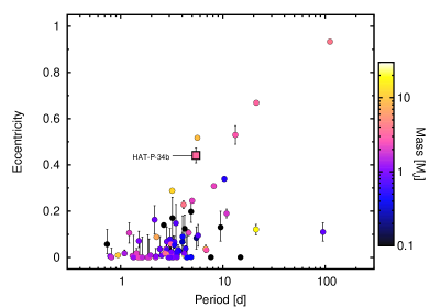
Figure 11.— Orbital-period–eccentricity diagram of TEPs with eccentricity uncertainty less than $0.1$. The color (greyscale shade) of the symbols indicates the mass of each planet. HAT-P-34b is labelled. As expected from tidal evolution theory, high eccentricity planets tend to have longer orbital periods and greater masses.

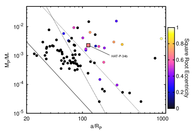
Figure 12.— A “tidal” diagram following Fig. 3 of Pont et al. (2011). The color (greyscale shade) of the symbols indicates the eccentricity, we assume zero eccentricity for planets that have a measured eccentricity within 4$\sigma$ of zero. The dotted line shows the locus of points with a circularization time-scale of 1 Gyr assuming small eccentricity, $Q_{P}=10^{6}$, and $P=3$ d. The thick solid line shows the relation $a=2a_{H}$ where $a_{H}$ is the semi-major axis at which the radius of the planet equals its Hill radius. The thin solid line shows $a=4a_{H}$.

With this in mind we conclude that the circularization of HAT-P-34b’s orbit is likely dominated by the tidal dissipation in the planet and using $Q_{P}=10^{6}$ and the expression for the tidal circularization timescale from Adams and Laughlin (2006), we estimate the eccentricity of HAT-P-34b should decay on the scale of 2Gyr, i.e. it is not in conflict with theoretical expectations. The possible outer companion indicated by the RV trend may also be responsible for pumping the eccentricity of the inner planet HAT-P-34b (see Correia et al., 2011 for a discussion).

Figure 11 shows HAT-P-34b on the orbital period–eccentricity plane of TEPs with well determined parameters (using our own compilation that attempts to keep up with various refinements to these parameters). It is apparent that eccentricity is correlated with orbital period and with planet mass, as expected from tidal theory. HAT-P-34b lies in a sparse position in these diagrams; for example, it has a high eccentricity for its period, the only similar planet being HAT-P-2b.

Figure 12 is a “tidal” plot (see Fig. 3 of Pont et al., 2011), showing TEPs with well measured properties in the $a/R_{p}$–$M_{p}/M_{\star}$ plane, using more data points (including the present discoveries) than Pont et al. (2011). Since $\tau_{c}=(4/63)Q_{P}\sqrt{(a^{3}/GM_{\star}}(a/R_{P})^{5}M_{p}/M_{\star}$, we expect planets with small relative semi-major axis ($a/R_{P}$) or planets with small relative mass ($M_{p}/M_{\star}$) to be circularized. This is indeed the case, as shown by the intensity (color) scale representing eccentricity. For hot Jupiters that migrate in by circularization of an initially very eccentric orbit, the expected “parking distance” is $\sim 2a_{H}$ (Ford and Rasio, 2006), where $a_{H}$ is the semi-major axis at which the radius of the planet equals its Hill radius. The thick solid line in Figure 12 shows this relation. A fairly good match for the dividing line between the circularized (denoted by black points) and eccentric (grey or color) points is at $a\approx 4a_{H}$ (marked with a thin solid line). This relation now includes very small mass Kepler discoveries. HAT-P-34b belongs to the sparse group of high relative semi-major axis ($a/R_{p}$) and massive extrasolar planets.

Appendix A Spectroscopic and Photometric Data

The following tables present the spectroscopic data (radial velocities, bisector spans, and activity index measurements) and high precision photometric data for the four planets presented in this paper.

Table 7 Relative radial velocities, bisector spans, and activity index measurements of HAT-P-34.

BJD	RV	$\sigma_{\rm RV}$	BS	$\sigma_{\rm BS}$	S	Phase	Instrument
(2,454,000$+$)	($\rm m\,s^{-1}$)	($\rm m\,s^{-1}$)	($\rm m\,s^{-1}$)	($\rm m\,s^{-1}$)
$1339.92722$	$-158.62$	$50.92$	$\cdots$	$\cdots$	$\cdots$	$0.188$	Subaru
$1339.93516$	$-201.37$	$57.36$	$\cdots$	$\cdots$	$\cdots$	$0.190$	Subaru
$1339.94290$	$-204.06$	$44.53$	$\cdots$	$\cdots$	$\cdots$	$0.191$	Subaru
$1341.11630$	$-246.80$	$47.11$	$\cdots$	$\cdots$	$\cdots$	$0.406$	Subaru
$1341.12058$	$-204.87$	$47.32$	$\cdots$	$\cdots$	$\cdots$	$0.407$	Subaru
$1341.12485$	$-193.24$	$43.00$	$\cdots$	$\cdots$	$\cdots$	$0.408$	Subaru
$1374.12069$	$-196.46$	$11.37$	$-2.85$	$6.57$	$0.176$	$0.459$	Keck
$1374.85735$	$\cdots$	$\cdots$	$-9.20$	$4.18$	$0.173$	$0.594$	Keck
$1374.86800$	$-80.49$	$11.89$	$-25.52$	$9.34$	$0.176$	$0.596$	Keck
$1375.95203$	$285.94$	$10.24$	$-15.73$	$4.46$	$0.178$	$0.795$	Keck
$1378.12823$	$-265.18$	$12.71$	$-13.52$	$7.86$	$0.174$	$0.194$	Keck
$1379.07458$	$-226.26$	$12.73$	$-10.85$	$3.72$	$0.176$	$0.368$	Keck
$1379.56536$	$-162.68$	$61.60$	$\cdots$	$\cdots$	$\cdots$	$0.458$	FIES
$1380.13344$	$-135.85$	$13.51$	$60.87$	$20.44$	$0.180$	$0.562$	Keck
$1380.49378$	$3.45$	$58.70$	$\cdots$	$\cdots$	$\cdots$	$0.628$	FIES
$1381.11125$	$110.87$	$14.71$	$-9.04$	$12.64$	$0.175$	$0.741$	Keck
$1381.55600$	$269.57$	$46.50$	$\cdots$	$\cdots$	$\cdots$	$0.823$	FIES
$1383.47949$	$-108.72$	$56.00$	$\cdots$	$\cdots$	$\cdots$	$0.176$	FIES
$1384.48968$	$-173.76$	$50.60$	$\cdots$	$\cdots$	$\cdots$	$0.361$	FIES
$1400.85414$	$-141.78$	$15.43$	$27.38$	$7.53$	$0.167$	$0.362$	Keck
$1403.82567$	$497.16$	$15.18$	$38.35$	$6.14$	$0.173$	$0.907$	Keck
$1404.83902$	$4.37$	$14.05$	$0.79$	$7.25$	$0.174$	$0.093$	Keck
$1415.04513$	$310.06$	$14.03$	$2.76$	$8.29$	$0.168$	$0.965$	Keck
$1423.66787$	$-115.78$	$78.50$	$\cdots$	$\cdots$	$\cdots$	$0.546$	FIES
$1424.64318$	$41.31$	$139.40$	$\cdots$	$\cdots$	$\cdots$	$0.725$	FIES
$1425.57489$	$474.54$	$48.70$	$\cdots$	$\cdots$	$\cdots$	$0.896$	FIES
$1426.64513$	$-154.35$	$57.60$	$\cdots$	$\cdots$	$\cdots$	$0.092$	FIES
$1464.85484$	$-99.38$	$15.03$	$-11.41$	$11.10$	$0.164$	$0.100$	Keck
$1465.94874$	$-249.34$	$13.70$	$-19.33$	$6.92$	$0.163$	$0.300$	Keck
$1467.71998$	$0.98$	$13.61$	$-12.70$	$8.00$	$0.164$	$0.625$	Keck

Note. — Note that for the iodine-free template exposures we do not measure the RV but do measure the BS and S index. Such template exposures can be distinguished by the missing RV value.

Table 8 Relative radial velocities, bisector spans, and activity index measurements of HAT-P-35.

Note. — Note that for the iodine-free template exposures we do not measure the RV but do measure the BS and S index. Such template exposures can be distinguished by the missing RV value.

Table 9 Relative radial velocities, bisector spans, and activity index measurements of HAT-P-36.

Table 10 Relative radial velocities, bisector spans, and activity index measurements of HAT-P-37.

Table 11 High-precision differential photometry of HAT-P-34.

Note. — This table is available in a machine-readable form in the online journal. A portion is shown here for guidance regarding its form and content.

Table 12 High-precision differential photometry of HAT-P-35.

Note. — This table is available in a machine-readable form in the online journal. A portion is shown here for guidance regarding its form and content.

Table 13 High-precision differential photometry of HAT-P-36.

Note. — This table is available in a machine-readable form in the online journal. A portion is shown here for guidance regarding its form and content.

Table 14 High-precision differential photometry of HAT-P-37.

Note. — This table is available in a machine-readable form in the online journal. A portion is shown here for guidance regarding its form and content.

References

- Adams and Laughlin (2006) Adams, F. C., & Laughlin, G. 2006, ApJ, 649, 1004
- Bakos et al. (2004) Bakos, G. Á., Noyes, R. W., Kovács, G., Stanek, K. Z., Sasselov, D. D., & Domsa, I. 2004, PASP, 116, 266
- Bakos et al. (2007a) Bakos, G. Á., et al. 2007a, ApJ, 670, 826
- Bakos et al. (2007b) Bakos, G. Á., et al. 2007b, ApJ, 671, L173
- Bakos et al. (2010) Bakos, G. Á., et al. 2010, ApJ, 710, 1724
- Bodenheimer, Laughlin, & Lin (2003) Bodenheimer, P., Laughlin, G., & Lin, D. N. C. 2003, ApJ, 592, 555
- Bonomo et al. (2010) Bonomo, A. S., et al. 2010, A&A, submitted
- Borucki et al. (2011) Borucki, W. J., et al. 2011, ApJ, 736, 19
- Bouchy et al. (2004) Bouchy, F., Pont, F., Santos, N. C., Melo, C., Mayor, M., Queloz, D., & Udry, S. 2004, A&A, 421, L13
- Bouchy et al. (2005) Bouchy, F., et al. 2005, A&A, 444, L15
- Buchhave et al. (2010) Buchhave, L. A., et al. 2010, ApJ, 720, 1118
- Burke et al. (2008) Burke, C. J., et al. 2008, ApJ, 686, 1331
- Butler et al. (1996) Butler, R. P. et al. 1996, PASP, 108, 500
- Carpenter (2001) Carpenter, J. M. 2001, AJ, 121, 2851
- Claret (2004) Claret, A. 2004, A&A, 428, 1001
- Cegla et al. (2012) Cegla, H. M., et al. 2012, MNRAS, 421, L54
- Claret & Cunha (1997) Claret, A.,& Cunha, N. C. S. 1997, A&A, 318, 187
- Correia et al. (2011) Correia, A. C. M., Boué, G., & Laskar, J. 2011, ApJL in press, arXiv:1111.5486
- Deleuil et al. (2012) Deleuil, M., et al. 2012, A&A, 538, A145
- Djupvik & Andersen (2010) Djupvik, A. A., & Andersen, J. 2010, in “Highlights of Spanish Astrophysics V” eds. J. M. Diego, L. J. Goicoechea, J. I. González-Serrano, & J. Gorgas (Springer: Berlin), p. 211
- Droege et al. (2006) Droege, T. F., Richmond, M. W., & Sallman, M. 2006, PASP, 118, 1666
- Ford and Rasio (2006) Ford, E. B., & Rasio, F. A. 2006, ApJ, 638, L45
- Fűrész (2008) Fűrész, G. 2008, Ph.D. thesis, University of Szeged, Hungary
- Goldreich & Soter (1966) Goldreich, P., & Soter, S. 1966, Icarus, 5, 375
- Hansen & Barman (2007) Hansen, B. M. S., & Barman, T. 2007, ApJ, 671, 861
- Hartman et al. (2009) Hartman, J. D., et al. 2009, ApJ, 706, 785
- Hartman et al. (2011a) Hartman, J. D., Bakos, G. Á., Kipping, D. M., et al. 2011a, ApJ, 728, 138
- Hartman et al. (2011b) Hartman, J. D., Bakos, G. Á., Torres, G., et al. 2011b, ApJ, 742, 59
- Hébrard et al. (2010) Hébrard, G., Désert, J.-M., Díaz, R. F., et al. 2010, A&A, 516, A95
- Hébrard et al. (2011) Hébrard, G., Evans, T. M., Alonso, R. 2011, A&A, 533, A130
- Hellier et al. (2009) Hellier, C., et al. 2009, Nature, 460, 1098
- Hellier et al. (2011) Hellier, C., Anderson, D. R., Collier-Cameron, A., Miller, G. R. M., Queloz, D., Smalley, B., Southworth, J., & Triaud, A. H. M. J. 2011, ApJ, 730, L31
- Howard et al. (2010) Howard, A. W., et al. 2010, ApJ, 721, 1467
- Howard et al. (2011) Howard, A. W., Marcy, G. W., Bryson, S. T., et al. 2011, arXiv:1103.2541
- Isaacson & Fischer (2010) Isaacson, H., & Fischer, D. 2010, ApJ, 725, 875
- Johnson et al. (2009) Johnson, J. A., Winn, J. N., Albrecht, S., Howard, A. W., Marcy, G. W., & Gazak, J. Z. 2009, PASP, 121, 1104
- Johnson et al. (2011) Johnson, J. A., Winn, J. N., Bakos, G. Á., et al. 2011, ApJ, 735, 24
- Kovács et al. (2002) Kovács, G., Zucker, S., & Mazeh, T. 2002, A&A, 391, 369
- Kovács et al. (2005) Kovács, G., Bakos, G. Á., & Noyes, R. W. 2005, MNRAS, 356, 557
- Kovács et al. (2010) Kovács, G., Bakos, G. á., Hartman, J. D., et al. 2010, ApJ, 724, 866
- Kurucz (2005) Kurucz, R. L. 2005, Memorie della Societa Astronomica Italiana Supplementi, 8, 14
- Lasker et al. (2008) Lasker, B. M., et al. 2008, AJ, 136, 735
- Latham et al. (2009) Latham, D. W., et al. 2009, ApJ, 704, 1107
- Latham et al. (2011) Latham, D. W., Rowe, J. F., Quinn, S. N., et al. 2011, ApJ, 732, L24
- Lissauer et al. (2011) Lissauer, J. J., Ragozzine, D., Fabrycky, D. C., et al. 2011, ApJS, 197, 8
- Madhusudhan & Winn (2009) Madhusudhan, N., & Winn, J. N. 2009, ApJ, 693, 784
- Makarov et al. (2009) Makarov, V. V., Beichman, C. A., Catanzarite, J. H., Fischer, D. A., Lebreton, J., Malbet, F., & Shao, M. 2009, ApJ, 707, L73
- Mandel & Agol (2002) Mandel, K., & Agol, E. 2002, ApJ, 580, L171
- Marcy & Butler (1992) Marcy, G. W., & Butler, R. P. 1992, PASP, 104, 270
- Martínez-Arnáiz et al. (2010) Martínez-Arnáiz, R., Maldonado, J., Montes, D., Eiroa, C., & Montesinos, B. 2010, A&A, 520, A79
- Maxted et al. (2010) Maxted, P. F. L, Anderson, D. R., Collier Cameron, A., et al. 2010, PASP, 122, 1465
- McLaughlin (1924) McLaughlin, D. B. 1924, ApJ, 60, 22
- Meibom & Mathieu (2005) Meibom, S., & Mathieu, R. D. 2005, ApJ, 620, 970
- Noguchi et al. (2002) Noguchi, K., et al. 2002, PASJ, 54, 855
- Noyes et al. (1984) Noyes, R. W., Hartmann, L. W., Baliunas, S. L., Duncan, D. K., & Vaughan, A. H. 1984, ApJ, 279, 763
- Noyes et al. (2008) Noyes, R. W., et al. 2008, ApJ, 673, L79
- O’Donovan et al. (2007) O’Donovan, F. T., et al. 2007, ApJ, 663, L37
- Ogilvie & Lin (2004) Ogilvie, G. I., & Lin, D. N. C. 2004, ApJ, 610, 477
- Pál (2009a) Pál, A. 2009a, MNRAS, 396, 1737
- Pál (2009b) Pál, A. 2009b, PhD thesis, Department of Astronomy, Eőtvős Loránd University, arXiv:0906.3486
- Pál et al. (2010) Pál, A., et al. 2010, MNRAS, 401, 2665
- Penev & Sasselov (2011) Penev, K., & Sasselov, D. 2011, ApJ, 731, 67
- Pollacco et al. (2008) Pollacco, D., et al. 2008, MNRAS, 385, 1576
- Pont et al. (2011) Pont, F., Husnoo, N., Mazeh, T., & Fabrycky, D. 2011, MNRAS, 414, 1278
- Queloz et al. (2001) Queloz, D. et al. 2001, A&A, 379, 279
- Quinn et al. (2010) Quinn, S. N., et al. 2010, ApJ, submitted, arXiv:1008.3565
- Rauer (2011) Rauer, H. 2011, in “Detection and Dynamics of Transiting Exoplanets, St. Michel l’Observatoire, France”, Edited by F. Bouchy; R. Díaz; C. Moutou; EPJ Web of Conferences, Volume 11, id.07001, 11, 7001
- Rossiter (1924) Rossiter, R. A. 1924, ApJ, 60, 15
- Saar et al. (2003) Saar, S. H., Hatzes, A., Cochran, W., & Paulson, D. 2003, The Future of Cool-Star Astrophysics: 12th Cambridge Workshop on Cool Stars, Stellar Systems, and the Sun , 12, 694
- Sato et al. (2002) Sato, B., Kambe, E., Takeda, Y., Izumiura, H., & Ando, H. 2002, PASJ, 54, 873
- Sato et al. (2005) Sato, B., et al. 2005, ApJ, 633, 465
- Schlaufman (2010) Schlaufman, K. C. 2010, ApJ, 719, 602
- Schneider et al. (2011) Schneider, J., Dedieu, C., Le Sidaner, P., Savalle, R., & Zolotukhin, I. 2011, A&A, 532, A79
- Skrutskie et al. (2006) Skrutskie, M. F., et al. 2006, AJ, 131, 1163
- Smalley et al. (2010) Smalley, B., Anderson, D. R., Collier Cameron, A., et al. 2010, A&A, 520, A56
- Sozzetti et al. (2007) Sozzetti, A. et al. 2007, ApJ, 664, 1190
- Torres et al. (2007) Torres, G. et al. 2007, ApJ, 666, 121
- Udalski et al. (2008) Udalski, A., et al. 2008, A&A, 482, 299
- Valenti & Fischer (2005) Valenti, J. A., & Fischer, D. A. 2005, ApJS, 159, 141
- Valenti & Piskunov (1996) Valenti, J. A., & Piskunov, N. 1996, A&AS, 118, 595
- Vaughan, Preston & Wilson (1978) Vaughan, A. H., Preston, G. W., & Wilson, O. C. 1978, PASP, 90, 267
- Vogt et al. (1994) Vogt, S. S. et al. 1994, Proc. SPIE, 2198, 362
- Winn et al. (2010) Winn, J. N., Fabrycky, D., Albrecht, S., & Johnson, J. A. 2010, ApJ, 718, L145
- Wright et al. (2011) Wright, J. T., et al. 2011, PASP, 123, 412
- Yi et al. (2001) Yi, S. K. et al. 2001, ApJS, 136, 417
- Zahn & Bouchet (1989) Zahn, J.-P., & Bouchet, L. 1989, A&A, 223, 112
- Zahn (1989) Zahn, J.-P. 1989, A&A, 220, 112
- Wright (2005) Wright, J. T. 2005, PASP, 117, 657