A proposal of a local modified QCD

Abstract

A local and renormalizable version of a modified PQCD introduced in previous works is presented. The construction indicates that it could be equivalent to massless QCD. The case in which only quark condensate effects are retained is discussed in more detail. Then, the appearing auxiliary fermion fields can be integrated leading to a theory with the action of massless QCD, to which one local and gauge invariant Lagrangian term for each quark flavour is added. These terms are defined by two gluon and two quark fields, in a form curiously not harming power counting renormalizability. The gluon self-energy is evaluated in second order in the gauge coupling and all orders in the new quark couplings, and the result became transversal as required by the gauge invariance. The vacuum energy was calculated in the two loop approximation and also became gauge parameter independent. The possibilities that higher loop contributions to the vacuum energy allow the generation of a quark mass hierarchy as a flavour symmetry breaking effect are discussed. However, the decision on this issue needs the evaluation of more than two loop contributions, in which more than one type of quark loops start appearing, possibly leading to interference effects in the vacuum energy.

I Introduction

The understanding of the hierarchy of quark masses is a fundamental open problem of High Energy Physics. In the investigation of this question, the theory of particle condensation in field theory had been a basic framework nambu ; fritzsch ; nilles ; fritzsch1 ; bardeen ; coleman ; miransky ; minkowski ; clague ; shifman ; fukuda ; celenza ; roberts ; pavel . In an effort to explore this issue, an alternative to the standard PQCD, including the presence of quark and gluon condensates in the free vacuum state generating the Wick expansion, has been considered in Refs. mpla ; prd ; epjc ; epjc1 ; jhep ; epjc2 ; epjc19 ; ana ; hoyer ; hoyer1 ; hoyer2 .  The exploration was in great extent motivated by the consideration about that massless QCD convey the strongest forces in Nature, as well as the free theory is a massless highly degenerate one for both quarks and gluons. This fact rises question about what could be the real intensity of the dimensional transmutation effect coleman .  The first step was to search for simple states of the free theory in which large numbers of zero momentum quark and gluon states were created in the standard free vacuum state, on which, then, adiabatically connect the interaction prd ; jhep ; epjc . In the start, the objective was to determine a modification of the standard Feynman rules of QCD embodying new condensate effects, with the expectation of to attain a theoretical prediction of superconductivity kind of properties of the particle mass spectrum underlined in Refs. fritzsch ; fritzsch1 .

In Refs.  mpla ; prd ; epjc ; epjc1 ; jhep ; epjc2 ; epjc19 ; ana , some indications about the possible dynamic generation of quark and gluon condensates were obtained. In particular in Ref. ana  it was  restricted the study to consider only the existence of quark condensates, with the aim of exploring the generation of large values for them. The motivation was the suspicion about that this mechanism might be able in generating a variant of the $top$ quark model, as an effective action for massless QCD.  In this case, the generating functional $Z$ of the system introduced in Ref.epjc19 was transformed to an alternative representation in which all the effects of the condensates were incorporated in a new vertex showing two quark and two gluon legs. This representation implemented the dimensional transmutation effect produced by the modification done in the free vacuum state.  The results suggested a technical path that could evidence a possible strong instability of massless QCD under the generation of fermion condensates. This outcome could furnish an explanation of the particle mass hierarchy in a kind of generalized  Nambu-Jona Lasinio dynamical symmetry mechanism nambu ; fritzsch ; bardeen ; miransky . However, a drawback of the diagram expansion introduced in Ref. ana was that the new vertex, although being covariant was a nonlocal one. That is, it was not associated to the four appearing fields defined at the same space-time point. Moreover, the evaluated two loop corrections to the vacuum energy turned out to be unbounded from below as a function of the quark condensate parameter, a fact that shifted the answer of the question about the prediction of dynamical mass generation to higher loop evaluations.   The undesirable properties of the new vertex,  can be traced back to the form of initial state of the free theory employed to connect the gauge interaction. This wavefunction was a sort squeezed state constructed with nearly zero momentum quark creations operators acting on the standard free vacuum. It has a structure similar to the BCS state in the usual superconductivity theory. The vertex was derived from a particular representation in which the Feynman gauge was explicitly employed and the quark free particle states used in the construction were particular zero momentum states in this special gauge. Therefore, the gauge invariance of the description was directly broken by the derivation. Henceforth, it came to the mind the possibility that the connection of the interaction on a specially defined in a more sophisticated way vacuum state could implement the locality and gauge invariance of the functional integral action in the ending theory. In particular coordinate dependent states in this same gauge exist that can be imagined to allow the mentioned construction.

In this work we start form a the results for the generating functional  for the massless QCD in which quark and gluon condensate parameters were introduced in the free vacuum, for afterwards construct the Wick expansion in Ref. epjc19 .  The resulting scheme included integrals over auxiliary boson and fermion parameters which appeared in the process of linearly representing the quadratic forms in the sources introduced by the inclusion of the gluon and quark condensates.  Then, it is firstly observed that the simple promotion of the gluon and quark condensate parameters to be space dependent functions  makes the action defining the generating functional a local and gauge invariant one.  Further, arguments are presented suggesting that the connection of the interaction in some sort of more general and yet undetermined initial modified vacuum state, could show the functional to be equivalent to massless QCD, after the adiabatic connection of the interaction.  Afterwards, the discussion in the work is restricted to the case of  retaining only the fermion condensate auxiliary functions.  The study of the case of the gluon condensate functions has also appreciable interest in itself for to explore its possibilities in the description of confinement and low energy Physics.  However, the issue of the quark mass generation possibility is closer to the fermion condensate parameters and we decided to consider it first here.   In this case, the Gaussian dependence of the quark auxiliary functions can be integrated out to give a theory action given by the massless QCD one plus six terms (one for each quark flavour). They implement the above mentioned local and gauge completions of the non local and gauge non invariant action obtained in Ref. ana .

The strongest support we had found for the physical relevance of these new terms simply comes form their structure; it seems that they are allowed counterterms of the massless QCD Lagrangian. In other words, if not obstructed by a subtle point not noticed by us, it seems that such a contributions can appears in the effective action of massless QCD after finite renormalizations of the four legs 1PI vertex determining the two gluon and two fermion fields terms in this expansion. Curiously, the new terms does not obstacle power counting renormalizability. This apparently strange property can be understood by taking into account that the new Lagrangian term also includes a contribution to the quark free propagators, which acquire a more converging behaviour $1/p^{2}$ at large momenta. Thus, the theory remains being power counting renormalizable. The above mentioned properties furnish an intrinsic interest to the theory resulting after simply adding the new local and renormalizable terms to the massless QCD action, as an alternative to the standard QCD.

Further, the Feynman diagrams associated to the new vertices and quark propagators are defined. As before noticed masses for the free fermions are defined by the new coupling constants associated to each of them. One curious outcome is that the larger the coupling (to be called from now on ”flavour condensate” couplings) associated to the action terms for each flavour, the smaller the quark mass becomes. That is, the top quark shows the smaller condensate coupling. The modified Feynman rules determined by the new vertices are defined. The gluon free propagator remains unaltered, but the fermion ones decompose in two terms showing the same massive pole. One of them resembles a scalar particle propagator and the other shows a Dirac propagator structure but including the same massive pole in addition to the usual zero mass one. We postpone the study of the renormalization (the behaviour of the running strong and flavour condensate couplings) and start here to explore the first implications of the analysis by evaluating the gluon self-energy in the $g^{2}$ order in the gauge coupling and all order in the flavour condensate ones. The result for the gluon polarization operator became transversal as implied by the gauge invariance for this second order in the coupling calculation when all orders of the flavour couplings are included. Further, the transversal part of the polarization operator is employed to evaluate the vacuum potential (taking all the mean field values equal to zero) as a function of the flavour condensate couplings. The potential in this case, at variance with the one evaluated in ana resulted to be bounded from below. Moreover, for small coupling values, in the here considered approximation, it shows a dynamical symmetry breaking generating non vanishing values for the quark masses. Since the renormalization group properties of the theory are delayed to a next study, it is not possible to make here clear cut phenomenological predictions. However, as a first exploration, the results for the potential were employed to select the $g$ coupling and the dimensional regularization scale parameter $\mu$ in order to fix the mass for the top quark nearly to 173 $GeV$. That is, the flavour condensate couplings are suggested as playing a role similar to a Higgs field in the approach. In this calculation the values of the coupling $g^{2}$ and the scale parameter $\mu$ result to be far from satisfying the known connection between the QCD running coupling and $\mu$. However, it can be taken into account that in the considered two loop calculation, all the six quark contributions are ”uncoupled”. That is, all propagator entering a diagram have the same flavour. Therefore, the hierarchy of quark masses, if really implied by the theory, as we currently suspect, is to be expected only after including higher loop terms in the potential. In this case mixing among different quark species has the chance of determining a realistic dynamical symmetry breaking effect. This view about the need of including higher loop corrections coincides with the one exposed in Ref. jhep , where it was remarked that this requirement becomes a natural one in a situation in which bound state effects are needed in determining a breaking of the flavour symmetry. In our considered case, to predict the quark mass hierarchy, it should occurs that a minimal effective potential appears for a large value of a single flavour quark condensate, while the other ones become very much smaller in size, and this minimum lays below another possible one in which various quarks condensate couplings get equal values. This situation only could have the chance of happening for the considered expansion, when the potential includes terms in which different sorts of quark propagators are present. Therefore, it is possible to conclude that the low values of the coupling got in the evaluation of the potential done here, is not yet reflecting a drawback for the analysis to be valid in describing the mass hierarchy. According to the above remarks, the next important steps in the search seems to be the study of the renormalization group properties of the expansion and the evaluation of three loops corrections to the potential for determining whether or not a quark mass hierarchy follows.

The presentation proceeds as follows.  In Section II the proposal of the local and renormalizable gauge theory including gluon and quark condensates and possibly being equivalent to massless QCD is presented. The case of retaining only the quark condensate is there shown to  reduce to a modified local and renormalizable massless QCD action. Section III is devoted to evaluate the gluon polarization operator in second order $g^{2}$ of the strong coupling and all orders in the flavour coupling parameters defining the new vertices, and to check its transversality. Finally, Section IV making use of the transversal part of the polarization operator, presents the evaluation of the effective potential in the two loop approximation and all orders in the new interaction parameters. In the Summary the results are reviewed and possible extensions of the work commented.

II A local and renormalizable modified QCD

Let us start by reviewing the main elements of the previous work which will be employed in the following discussion. The generating functional of massless QCD written in Euclidean variables as in Ref. epjc19  has the expression

$$Z[j,\eta,\overline{\eta},\xi,\overline{\xi}] =\frac{I[j,\eta,\overline{\eta},\xi,\overline{\xi}]}{I[0,0,0,0]},$$

$$I[j,\eta,\overline{\eta},\xi,\overline{\xi}] =\exp(V^{int}[\frac{\delta}{\delta j},\frac{\delta}{\delta\overline{\eta}},\frac{\delta}{-\delta\eta},\frac{\delta}{\delta\overline{\xi}}\frac{\delta}{-\delta\xi}]){\small\times}$$ (1)

$$\exp(\int\frac{dk}{(2\pi)^{D}}j(-k)\frac{1}{2}D(k)j(k)){\small\times}$$

$$\exp(\sum_{f}\int\frac{dk}{(2\pi)^{D}}\overline{\eta}_{f}(-k)G_{f}(k)\eta_{f}(k)){\small\times}$$

$$\exp(\int\frac{dk}{(2\pi)^{D}}\overline{\xi}(-k)G_{gh}(k)\xi(k)){\small,}$$

$$f =1,2,...6.$$ (2)

The functional is associated to the action $S_{g}$ depending on the gauge interaction coupling $g$.  $S_{0}$ for $g=0$ defines the free action. $S_{g}$ and the vertex part  Lagrangian $V^{int}$ are defined in terms of the six quark $\Psi_{f}$ ($f=1,...,6$), gluon $A$ and ghost $\chi$ fields in the form

$$S_{g} =\int dx(-\frac{1}{4}F_{\mu\nu}^{a}F_{\mu\nu}^{a}-\frac{1}{2\alpha}\partial_{\mu}A_{\mu}^{a}\partial_{\nu}A_{\nu}^{a}+\overline{c}^{a}\overleftarrow{\partial}_{\mu}D_{\mu}^{ab}c^{b}-\sum_{f}\overline{\Psi}_{f}^{i}\text{ }i\gamma_{\mu}D_{\mu}^{ij}\Psi_{f}^{j}),\text{ \ }$$ (3)

$$V^{int} =S_{g}-S_{0},$$ (4)

where the field intensity, and covariant derivatives follow the conventions

$$F_{\mu\nu}^{a} =\partial_{\mu}A_{\nu}^{a}-\partial_{\nu}A_{\mu}^{a}-gf^{abc}A_{\mu}^{b}A_{\nu}^{c},$$

$$D_{\mu}^{ij} =\partial_{\mu}\delta^{ij}+ig\text{ }A_{\mu}^{a}T_{a}^{ij},\ \ \ \ D_{\mu}^{ab}=\partial_{\mu}\delta^{ab}+gf^{abc}\text{ }A_{\mu}^{c},$$ (5)

$$\{\gamma_{\mu},\gamma_{\nu}\} =-2\delta_{\mu\nu},\ \ \ \ [T_{a}T_{b}]=if^{abc}T_{c}.$$

The gluon and quark condensate parameters representing the modified vacuum free state used to construct the Wick expansion enter the generating functional only though the free quark and gluon propagators, which have the forms

$$D_{\mu\nu}^{ab}(k) =\delta^{ab}(\frac{1}{k^{2}}(\delta_{\mu\nu}-(1-\alpha)\frac{k_{\mu}k_{\nu}}{k^{2}})\theta_{N}(k)+C_{g}\delta^{D}(k)\delta_{\mu\nu}),$$

$$G_{f}^{ij}(k) =\delta^{ij}{\large(}\frac{\theta_{N}(k)}{m+\gamma_{\mu}k_{\mu}}+C_{f}\delta^{D}(k)I{\large)},$$

$$G_{gh}^{ab}(k) =\delta^{ab}\frac{\theta_{N}(k)}{k^{2}}.$$ (6)

The derivation considered the possibility of quarks already having the mass $m$ appearing.  These  expressions are solutions of the tree approximation for the propagators, since the 4-dimensional Delta functions is a solution of the homogeneous Dirac and Klein-Gordon equations, because at zero momentum both equations vanish. As discussed in the  Ref. epjc1  , the functions $\theta_{N}(k)$ regularize all the propagators at zero value of the momentum as required by the gauge theory quantization nakanishi .  The notation of Ref. muta is closely followed along the work. The Einstein summation notation in the flavour indices is employed and a flavour (or other kind of index) between parenthesis means that it does not follow the Einstein convention.

In Refs. mpla ; prd ; epjc ; epjc1 ; jhep ; epjc2 ; epjc19 ; ana , the alternative form of the functional integral (1) for massless QCD was obtained after modifying the free vacuum, by creating in it gluons, quark and ghosts of nearly zero momentum. These changes of the initial condition in the process of connecting the interaction, after using the rules for constructing the Wick expansion (gasioro ),  led to modified free propagators in (6). Some quantities had been evaluated with these modified expansion (epjc1 ; jhep ; epjc2 ) and its general gauge invariance was argued epjc1 ; jhep ; epjc2 . It was possible to check that if the gluon condensate parameter defined here is chosen to match the estimated value of the more usual gluon condensation parameter $<g^{2}G^{2}>,$ then the masses of the light quarks are predicted to be the constituent quark mass of nearly $333$ MeV. In addition, sample loop calculations of the vacuum energy as a function of the condensate parameters were done in Refs. epjc1 ; jhep ; epjc2 , in one loop order or by employing the ladder approximations for the quark and gluon propagators. They gave indications of a dynamical generation of the quark and gluon condensates. For gluons the one loop result gave a form of the potential similar to the potential in the early chromomagnetic Savvidi models of confinement.

However, the working expression (1) of the generating functional shows two limitations, one of theoretical nature and another technical one. The technical one is associated with the fact that in the new contributions existed singularities requiring of  a special regularization process to be well defined epjc1 .  The theoretical one can be described as follows. In Ref. epjc19 we linearized the quadratic terms in the gluon and quark sources by means of introducing Gaussian integration over auxiliary fields. This led to a functional integral in which interesting dimensionally transmuted gluon and quark propagators already appeared. Next, in Ref. ana we restricted the discussion to the case in which only the quark condensate parameter were retained, seeking to transform the modified Feynman expansion in a more helpful form by integrating over the auxiliary parameters. It was possible to transform the generating functional by mapping the effect of the condensate, from incorporating a Delta function term in the free propagator, to the addition of a new term in the massless QCD action associated to a vertex, showing two gluon and two quark legs. However, the form of this vertex, although being Lorentz and global color invariant was not local in space-time, since it had the form of a double integral over the product of two pairs of fields evaluated at two different space-time points. This effect was a direct consequence of the particular Dirac Delta structure in the momentum space of the free propagator.

In this section we attempt to modified the construction of the modified expansion in order to overcome both of the problems. The starting idea for this purpose was suggested by the form of the generating functional obtained in Refs. epjc19 ; ana .  In beginning, let us consider the result for $Z$  given in Ref. epjc19 incorporating gluon as well as quark zero momentum condensates in the free ground state before connecting the interaction. The expression for $Z$ is given by Eq. (12) of Ref. epjc19 in the form

$$Z[j,\eta,\overline{\eta},\xi,\overline{\xi}] =\frac{I[j,\eta,\overline{\eta},\xi,\overline{\xi}]}{I[0,0,0,0]},$$

$$I[j,\eta_{f},\overline{\eta}_{f},\xi,\overline{\xi}] =\frac{1}{\mathcal{N}}\int\int d\alpha d\overline{\chi}d\chi\exp{\large[}-\sum_{f}\overline{\chi}_{f,u}^{i}\chi_{f,u}^{i}-\frac{\alpha_{\mu}^{a}\alpha_{\mu}^{a}}{2}{\large]}$$

$$\exp{\large[}V^{int}{\large[}\frac{\delta}{\delta j}{\small+(}\frac{2C_{g}}{(2\pi)^{D}}{\small)}^{\frac{1}{2}}{\small\alpha,}\frac{\delta}{\delta\overline{\eta}}{\small+(}\frac{C_{f}}{(2\pi)^{D}}{\small)}^{\frac{1}{2}}{\small\chi}_{f}{\small,}\frac{\delta}{-\delta\eta}{\small+(}\frac{C_{f}}{(2\pi)^{D}}{\small)}^{\frac{1}{2}}\overline{\chi}_{f}{\small,}\frac{\delta}{\delta\overline{\xi}}\frac{\delta}{-\delta\xi}{\small,\alpha,}\overline{\chi}{\small,\chi{\large]]}\times}$$ (7)

$$\exp{\large[}\int\frac{dk}{(2\pi)^{D}}{\Large(}{\small j(-k)}\frac{1}{2}{\small D}^{F}{\small(k)j(k)+}\sum_{f}\overline{\eta}_{f}{\small(-k)G}^{F}{\small(k)\eta}_{f}{\small(k)]+}\overline{\xi}{\small(-k)G}_{gh}^{F}{\small(k)\xi(k)]{\Large)}{\large]},}$$

$$\text{ }\chi =(\chi_{1},\chi_{2},...\chi_{f}...,\chi_{6}),\text{ \ \ }\overline{\chi}=(\overline{\chi}_{1},\overline{\chi}_{2},...\overline{\chi}_{f}...,\overline{\chi}_{6}),$$ (8)

$$d\alpha d\overline{\chi}d\chi ={\displaystyle\prod\limits_{a,\text{ }\mu}}d\alpha_{\mu}^{a}{\displaystyle\prod\limits_{f,\text{ }i,\text{ }r}}d\overline{\chi}_{f,\text{ }r}^{i}d\chi_{f,\text{ }r}^{i}.$$ (9)

where the vertex interaction Lagrangian $V^{int}$ is defined in (4) and in which the propagators for gluons, quarks and ghost fields are the usual Feynman ones as indicated by the superscript $F$.  The whole expression is a Gaussian mean value over the gluon and quark auxiliary parameters $\alpha,$ $\overline{\chi}$ ,$\chi$.  They are constants in coordinate space, $\alpha$ has Lorentz and color gluon indices and $\chi$ and $\overline{\chi}$ have spinor and quark color indices. Since the Delta function terms were linked with the zero momentum Fourier components of the sources, the number of auxiliary Gaussian variables required to represent in a linear form these zero momentum components of the sources is reduced to the small number of the indices of the internal field components.

Before continuing, let us rewrite the expression  for the vertex Lagrangian $V^{int}$ appearing in the above relation in order to discuss the coming points.  To simplify the writing let us define a notation absorbing the condensate coefficients in new defined parameters as follows

$$\phi_{\mu}^{a}={\small(}\frac{2C_{g}}{(2\pi)^{D}}{\small)}^{\frac{1}{2}}\alpha_{\mu}^{a},\text{ \ }\beta_{f,r}^{i}={\small(}\frac{C_{f}}{(2\pi)^{D}}{\small)}^{\frac{1}{2}}\chi_{f,r}^{i},\text{ \ }\overline{\beta}_{f,r}^{i}={\small(}\frac{C_{f}}{(2\pi)^{D}}{\small)}^{\frac{1}{2}}\overline{\chi}_{f,r}^{i}.$$

Now, let us call $S_{g}^{\ast}$ , $S_{0}^{\ast}$ the actions $S_{g}$ , $S_{0}$ after being evaluated in the shifted fields which define $V_{int}$ in the formula (7) through $V_{int}=S_{g}^{\ast}-S_{0}^{\ast}$.  These quantities, as expressed in terms of the fields and the above redefined condensate parameters, have the expressions

$$S_{g}^{\ast} =S_{g}{\small[}A{\small+(}\frac{2C_{g}}{(2\pi)^{D}}{\small)}^{\frac{1}{2}}{\small\alpha,}\Psi_{f}{\small+(}\frac{C_{f}}{(2\pi)^{D}}{\small)}^{\frac{1}{2}}{\small\chi}_{f}{\small,}\overline{\Psi}_{f}{\small+(}\frac{C_{f}}{(2\pi)^{D}}{\small)}^{\frac{1}{2}}\overline{\chi}_{f}{\small,}\frac{\delta}{\delta\overline{\xi}},\frac{\delta}{-\delta\xi}{\small]}$$

$$=\int dx{\Large[-}\frac{1}{4}F_{\mu\nu}^{a}(A+\phi)F_{\mu\nu}^{a}(A+\phi)$$

$$-\frac{1}{2\alpha}\partial_{\mu}A_{\mu}^{a}\partial_{\nu}A_{\nu}^{a}-\sum_{f}\overline{\Psi}_{f}^{i}\text{ }i\gamma_{\mu}D_{\mu}^{ij}\Psi_{f}^{j}-\overline{c}^{a}\partial_{\mu}D_{\mu}^{ab}(A+\phi)c^{b}$$

$$-\sum_{f}{\Large(}\overline{\Psi}_{f}^{i}\text{ }i\gamma_{\mu}D_{\mu}^{ij}(A+\phi)\Psi_{f}^{j}+\overline{\Psi}_{f}^{i}\text{ }i\gamma_{\mu}D_{\mu}^{ij}(A)\beta_{f}^{j}+\overline{\beta}_{q}^{i}\text{ }i\gamma_{\mu}D_{\mu}^{ij}(A)\Psi_{q}^{j}{\Large)}$$

$$-\sum_{f}{\Large(}\overline{\beta}_{f}^{i}\text{ }i\gamma_{\mu}\text{ }ig\phi_{\mu}^{a}T_{a}^{ij}\beta_{f}^{j}+$$

$$\overline{\Psi}_{f}^{i}\text{ }i\gamma_{\mu}\text{ }ig\phi_{\mu}^{a}T_{a}^{ij}\beta_{f}^{j}+\overline{\beta}_{f}^{i}\text{ }i\gamma_{\mu}\text{ }ig\text{ }\phi_{\mu}^{a}T_{a}^{ij}\Psi_{f}^{j}{\Large)],}$$ (10)

$$S_{0}^{\ast} =S_{0}{\small[}A{\small+(}\frac{2C_{g}}{(2\pi)^{D}}{\small)}^{\frac{1}{2}}{\small\alpha,}\Psi{\small+(}\frac{C_{f}}{(2\pi)^{D}}{\small)}^{\frac{1}{2}}{\small\chi}_{f}{\small,}\overline{\Psi}{\small+(}\frac{C_{f}}{(2\pi)^{D}}{\small)}^{\frac{1}{2}}\overline{\chi}_{f}{\small,}\frac{\delta}{\delta\overline{\xi}},\frac{\delta}{-\delta\xi}{\small]}$$

$$=\int dx\text{ }{\large[}-\frac{1}{4}(\partial_{\mu}A_{\nu}^{a}-\partial_{\nu}A_{\mu}^{a})(\partial_{\mu}A_{\nu}^{a}-\partial_{\nu}A_{\mu}^{a})-\frac{1}{2\alpha}\partial_{\mu}A_{\mu}^{a}\partial_{\nu}A_{\nu}^{a}-\overline{c}^{a}\partial^{2}c^{a}$$

$$-\sum_{f}\overline{\Psi^{i}}_{f}\text{ }i\gamma_{\mu}\partial_{\mu}\Psi_{f}^{i}{\large]}$$ (11)

One important point in the above expressions is related with the last two terms in $S_{g}^{\ast}.$ Note that these are the only  linear in the radiation fields terms appearing and that they vanish when the coupling is set to zero. Since the condensate auxiliary parameters are constants in space-time, it follows that these terms are just proportional to the zero momentum  Fourier components of the entering kind of radiation field. Therefore, when this terms are expressed in terms of the functional derivatives of the corresponding field sources, they are proportional to the functional derivative over the zero momentum component of the sources. Therefore, their action over the free generating functionals in  (7) vanish because the functionals are not depending of these components, thanks to the Nakanishi zero momentum regularization appearing factors in  (1).  Since the condensate auxiliary parameters are constants they do not appear in $S_{0}^{\ast}$ which due to the masslessness of the theory is defined by pure differential operators which action on them vanish.

Henceforth, the action to be employed in what follows is

$$S_{g}^{\ast} =S_{g}^{\ast}[A{\small,}\Psi{\small,}\overline{\Psi}{\small,}c,\overline{c},{\small\alpha,\chi,\overline{\chi}]}$$

$$=\int dx\text{ }{\Large[}-\frac{1}{4}F_{\mu\nu}^{a}(A+\phi)F_{\mu\nu}^{a}(A+\phi)$$

$$-\frac{1}{2\alpha}\partial_{\mu}A_{\mu}^{a}\partial_{\nu}A_{\nu}^{a}-\overline{c}^{a}\partial_{\mu}D_{\mu}^{ab}(A+\phi)c^{b})$$

$$-\sum_{f}{\large(}\overline{\Psi}_{f}^{i}\text{ }i\gamma_{\mu}D_{\mu}^{ij}(A+\phi)\Psi_{f}^{j}+\overline{\Psi}_{f}^{i}\text{ }i\gamma_{\mu}D_{\mu}^{ij}(A)\beta_{f}^{j}+\overline{\beta}_{f}^{i}\text{ }i\gamma_{\mu}D_{\mu}^{ij}(A)\Psi_{f}^{j}$$

$$+\overline{\beta}_{f}^{i}\text{ }i\gamma_{\mu}\text{ }ig\phi_{\mu}^{a}T_{a}^{ij}\beta_{f}^{j}{\large)}{\Large].}$$ (12)

These last properties are useful to obtain an alternative functional integral form for $Z$.  For this purpose consider the rewriting of this quantity as follows

$$Z[j,\eta,\overline{\eta},\xi,\overline{\xi}] =\frac{I[j,\eta,\overline{\eta},\xi,\overline{\xi}]}{I[0,0,0,0]},$$

$$I[j,\eta,\overline{\eta},\xi,\overline{\xi}] =\frac{1}{\mathcal{N}}\int\int d\alpha\text{ }d\overline{\chi}\text{ }d\chi\exp{\large[}-\sum_{f}\overline{\chi}_{f,u}^{i}\chi_{f,u}^{i}-\frac{\alpha_{\mu}^{a}\alpha_{\mu}^{a}}{2}{\large]}\times$$

$$\exp{\large[}S_{g}^{\ast}{\small[}\frac{\delta}{\delta j}{\small,}\frac{\delta}{\delta\overline{\eta}}{\small,}\frac{\delta}{-\delta\eta},\frac{\delta}{\delta\overline{\eta}},\frac{\delta}{-\delta\eta},\alpha,\chi,\overline{\chi}{\large]}{\small\times}$$

$$\exp{\large[}{\small-}S_{0}{\small[}\frac{\delta}{\delta j}{\small,}\frac{\delta}{\delta\overline{\eta}}{\small,}\frac{\delta}{-\delta\eta}{\small,}\frac{\delta}{\delta\overline{\xi}}\frac{\delta}{-\delta\xi}{\large]}{\small\times}$$

$$\exp{\large[}\int\frac{dk}{(2\pi)^{D}}{\Large(}{\small j(-k)}\frac{1}{2}{\small D}^{F}{\small(k)j(k)+}\sum_{f}\overline{\eta}_{f}{\small(-k)G}^{F}{\small(k)\eta}_{f}{\small(k)+}\overline{\xi}{\small(-k)G}_{gh}^{F}{\small(k)\xi(k)]{\Large)]},}$$ (13)

Then, by returning each of the free generating functions to their functional integral original expression giving rise to them, it follows the relation

$$\exp{\small[-}S_{0}{\small[}\frac{\delta}{\delta j}{\small,}\frac{\delta}{\delta\overline{\eta}}{\small,}\frac{\delta}{-\delta\eta}{\small,}\frac{\delta}{\delta\overline{\xi}},\frac{\delta}{-\delta\xi}{\small]\times}\int\mathcal{D}[A,\overline{\Psi},\Psi,\overline{c},c]$$

$$\exp{\small[}\int dx{\Large(}\mathcal{L}_{0}{\small[}A{\small,}\Psi{\small,}\overline{\Psi}{\small,}c,\overline{c}{\small]+j(x)A(x)+}\sum_{f}({\small\overline{\eta}}_{f}{\small(x)\Psi}_{f}{\small(x)+\overline{\Psi}}_{f}{\small(x)\eta}_{f}{\small(x)){\Large)}.}$$

$$=\int\mathcal{D}[A,\overline{\Psi},\Psi,\overline{c},c]\exp{\large[}\int dx\text{ }{\Large(}{\small\mathcal{L}_{0}[A,\Psi,\overline{\Psi},c,\overline{c}]-\mathcal{L}_{0}[A,\Psi,\overline{\Psi},c,\overline{c}]+j(x)A(x)+}\sum_{f}{\large(}{\small\overline{\eta}}_{f}{\small(x)\Psi}_{f}{\small(x)+\overline{\Psi}}_{f}{\small(x)\eta}_{f}{\small(x){\large)}{\Large)]}.}$$

$$=\int\mathcal{D}[A,\overline{\Psi},\Psi,\overline{c},c]\exp{\large[}\int dx\sum_{f}{\large(}{\small\overline{\eta}}_{f}{\small(x)\Psi}_{f}{\small(x)+\overline{\Psi}}_{f}{\small(x)\eta}_{f}{\small(x)}{\large)].}$$ (14)

Employing the above expression it follows for $Z$

$$Z[j,\eta,\overline{\eta},\xi,\overline{\xi}] =\frac{1}{\mathcal{N}}\int\int d\alpha d\overline{\chi}d\chi\exp[-\sum_{f}\overline{\chi}_{f,\text{ }r}^{i}\chi_{f,\text{ }r}^{i}-\frac{\alpha_{\mu}^{a}\alpha_{\mu}^{a}}{2}]$$

$$\exp{\large[}{\small S}_{g}^{\ast}{\small[\frac{\delta}{\delta j},\frac{\delta}{\delta\overline{\eta}},\frac{\delta}{-\delta\eta},\frac{\delta}{\delta\overline{\eta}},\frac{\delta}{-\delta\eta},\alpha,\chi,\overline{\chi}]{\large]}\times}$$ (15)

$$\int\mathcal{D}[A,\overline{\Psi},\Psi,\overline{c},c]\exp{\large[}\int dx\text{ }{\large(}{\small j(x)A(x)+\sum_{f}{\large(}\overline{\eta}_{f}(x)\Psi_{f}(x)+\overline{\Psi}_{f}(x)\eta_{f}(x){\large)}{\Large)}}{\large]}$$

$$=\frac{1}{\mathcal{N}}\int\int d\alpha d\overline{\chi}d\chi\exp{\large[}-\sum_{f}\overline{\chi}_{f,\text{ }r}^{i}\chi_{f,\text{ }r}^{i}-\frac{\alpha_{\mu}^{a}\alpha_{\mu}^{a}}{2}{\large]}\times$$

$$\int\mathcal{D}[A,\overline{\Psi},\Psi,\overline{c},c]\exp{\large[}\int dx\text{ }{\large(}S_{g}^{\ast}{\small[}A{\small,\Psi,}\overline{\Psi},c,\overline{c},\alpha,\chi,\overline{\chi}{\small]+}$$

$${\small j(x)A(x)+\sum_{f}{\large(}\overline{\eta}_{f}(x)\Psi_{f}(x)+\overline{\Psi}_{f}(x)\eta_{f}(x){\large))}{\Large{\large]}.}}$$

where the action $S_{g}^{\ast}$ takes the form

$$S_{g}^{\ast} =S_{g}^{\ast}[A{\small,}\Psi{\small,}\overline{\Psi}{\small,}c,\overline{c},{\small\alpha,\chi,\overline{\chi}]}$$

$$=\int dx{\large[}{\Large-}\frac{1}{4}F_{\mu\nu}^{a}(A+{\small(}\frac{2C_{g}}{(2\pi)^{D}}{\small)}^{\frac{1}{2}}\alpha_{\mu}^{a})F_{\mu\nu}^{a}(A+{\small(}\frac{2C_{g}}{(2\pi)^{D}}{\small)}^{\frac{1}{2}}\alpha_{\mu}^{a})$$

$$-\frac{1}{2\alpha}\partial_{\mu}A_{\mu}^{a}\partial_{\nu}A_{\nu}^{a}-\overline{c}^{a}\partial_{\mu}D_{\mu}^{ab}(A+{\small(}\frac{2C_{g}}{(2\pi)^{D}}{\small)}^{\frac{1}{2}}\alpha_{\mu}^{a})c^{b})$$

$$-\sum_{f}{\Large(}\overline{\Psi}_{f}^{i}\text{ }i\gamma_{\mu}D_{\mu}^{ij}(A+{\small(}\frac{2C_{g}}{(2\pi)^{D}}{\small)}^{\frac{1}{2}}\alpha_{\mu}^{a})\Psi_{f}^{j}+\overline{\Psi}_{f}^{i}\text{ }i\gamma_{\mu}D_{\mu}^{ij}(A)\chi_{f}^{j}{\small(}\frac{C_{f}}{(2\pi)^{D}}{\small)}^{\frac{1}{2}}+{\small(}\frac{C_{f}}{(2\pi)^{D}}{\small)}^{\frac{1}{2}}\overline{\chi}_{f}^{i}\text{ }i\gamma_{\mu}D_{\mu}^{ij}(A)\Psi_{f}^{j}$$

$$+{\small(}\frac{C_{f}}{(2\pi)^{D}}{\small)(}\frac{2C_{g}}{(2\pi)^{D}}{\small)}^{\frac{1}{2}}\overline{\chi}_{f}^{i}\text{ }i\gamma_{\mu}\text{ }ig\alpha_{\mu}^{a}T_{a}^{ij}\chi_{f}^{j}{\large)]}{\Large.}$$ (16)

This formula is exactly the same  that was obtained in Ref. ana  when the gluon condensate parameter vanishes. This can be seen more clearly after considering that all the derivatives of the quark auxiliary parameters vanish.  This alternative expression suggests that the above defined local and renormalizable modification of QCD has the chance of being equivalent to massless QCD.   For seeing this possibility it can be observed that the non locality and lack of gauge invariance of the theory defined by  Z, are just determined by the coordinate independence of the auxiliary variables.  In other words if $\overline{\chi}_{f}^{i}$, $\chi_{f}^{j}$ and $\alpha_{\mu}^{a}$ are formally considered as arbitrary functions of the coordinates, the action $S_{g}^{\ast}$ (after substracting from it the gauge fixing and the ghost terms) becomes gauge invariant under the gauge transformations

$$w(x) =\exp[-i\text{ }\lambda_{a}(x)T^{a}],$$

$$w_{ad}(x) =\exp[-i\text{ }\lambda_{a}(x)T_{ad}^{a}],\text{ \ \ \ }(T_{ad}^{a})^{ik}\equiv i\text{ }f\text{ }^{iak},$$

$$A_{\mu}^{\prime}(x) =w_{ad}A_{\mu}(x)w_{ad}^{-1}-\frac{i}{g}w_{ad}(x)\partial_{\mu}w_{ad}(x)^{-1},\text{ \ \ \ }$$

$$\Psi_{f}^{\prime}(x) =w(x)\Psi_{f}(x)w(x)^{-1},\overline{\Psi}_{f}^{\prime}(x)=w(x)\overline{\Psi}_{f}(x)w(x)^{-1},$$

$$c^{\prime}(x) =w_{ad}(x)c(x)w_{ad}(x)^{-1},\overline{c}^{\prime}(x)=w_{ad}(x)\overline{c}(x)w_{ad}(x)^{-1}$$

$$\phi_{\mu}^{\prime}(x) =w_{ad}(x)\phi_{\mu}(x)w_{ad}(x)^{-1},$$

$$\chi_{f} =w(x)\chi_{f}(x)w(x)^{-1},$$

$$\overline{\chi}_{f}^{{}^{\prime}} =w(x)\overline{\chi}_{f}^{i}(x)w(x)^{-1},$$ (17)

where the auxiliary functions (before being the parameters) are represented as elements of the SU(3) algebra. The boson fields like $A_{\mu}(x)=A_{\mu}^{a}(x)T_{ad}^{a},$ are expressed in terms of the adjoint representation for the algebra generators $T_{ad}^{a},$ (the subscript $ad$ indicates ”adjoint”) and the fermion quantities in the fundamental one in terms of the Gell-Mann matrices.

However, the constant in the coordinates character of the condensate parameters, followed as a direct consequence of the particular nature in which the modified free vacuum state including condensed zero momentum gluons and quarks was constructed.  Thus, it is possible to conceive a wide range of alternative ways of defining generalized modified free vacuum wavefunctions within the manifold of states annihilated by the BRST charge of the free problem.  Such a possibility, leads to the expectation about that a procedure  can be developed in which the ending outcome can be of the similar form as (15), but in which the  Gaussian integrations over the condensate parameters  become substituted by Gaussian functional integrations over condensate functions depending of the coordinates.   We had attempted to determine such an alternative procedure, which validity will shows that the modified theory is in fact equivalent to massless QCD, but up to now we had not been able to find it.    In this work however, we simply will propose the generalized expansion and consider the first implications of the local gauge invariant alternative forms of QCD that they represent.

Therefore, we propose the following expression for the generating functional of a local and renormalizable gauge theory  which, as it was argued above, has the chance of reflecting nonperturbative properties of massless QCD

$$Z[j,\eta,\overline{\eta},\xi,\overline{\xi}] =\frac{1}{\mathcal{N}}\int\int\mathcal{D}[\alpha,\overline{\chi},\chi]\exp[-\sum_{f}\overline{\chi}_{f,\text{ }r}^{i}(x)\chi_{f,\text{ }r}^{i}(x)-\frac{\alpha_{\mu}^{a}(x)\alpha_{\mu}^{a}(x)}{2}]\times$$

$$\int\mathcal{D}[A,\overline{\Psi},\Psi,\overline{c},c]\exp{\large[}\int dx\text{ }{\large(}S_{g}^{\ast}{\small[}A{\small,\Psi,}\overline{\Psi},c,\overline{c},\alpha,\chi,\overline{\chi}{\small]+}$$

$${\small j(x)A(x)+}\sum_{f}{\large(}{\small\overline{\eta}}_{f}{\small(x)\Psi}_{f}{\small(x)+\overline{\Psi}}_{f}{\small(x)\eta}_{f}{\small(x){\large))]}},$$ (18)

in which the action is defined by

$$S_{g}^{\ast} =S_{g}^{\ast}[A{\small,}\Psi{\small,}\overline{\Psi}{\small,}c,\overline{c},{\small\alpha,\chi,\overline{\chi}]}$$

$$=\int dx{\Large[}-\frac{1}{4}F_{\mu\nu}^{a}(A+{\small(}\frac{2C_{g}}{(2\pi)^{D}}{\small)}^{\frac{1}{2}}\alpha_{\mu}^{a})F_{\mu\nu}^{a}(A+{\small(}\frac{2C_{g}}{(2\pi)^{D}}{\small)}^{\frac{1}{2}}\alpha_{\mu}^{a})$$

$$-\frac{1}{2\alpha}\partial_{\mu}A_{\mu}^{a}\partial_{\nu}A_{\nu}^{a}-\overline{c}^{a}\partial_{\mu}D_{\mu}^{ab}(A+{\small(}\frac{2C_{g}}{(2\pi)^{D}}{\small)}^{\frac{1}{2}}\alpha_{\mu}^{a})\text{ }c^{b})$$

$$-\sum_{f}\overline{\Psi}_{f}^{i}\text{ }i\gamma_{\mu}D_{\mu}^{ij}(A+{\small(}\frac{2C_{g}}{(2\pi)^{D}}{\small)}^{\frac{1}{2}}\alpha_{\mu}^{a})\text{ }\Psi_{f}^{j}$$

$$-\sum_{f}\overline{\Psi}_{f}^{i}\text{ }i\gamma_{\mu}D_{\mu}^{ij}(A)\chi_{f}^{j}\text{ }{\small(}\frac{C_{f}}{(2\pi)^{D}}{\small)}^{\frac{1}{2}}-\sum_{f}{\small(}\frac{C_{f}}{(2\pi)^{D}}{\small)}^{\frac{1}{2}}\overline{\chi}_{f}^{i}\text{ }i\gamma_{\mu}D_{\mu}^{ij}(A)\Psi_{f}^{j}$$

$$-\sum_{f}{\small(}\frac{C_{f}}{(2\pi)^{D}}{\small)(}\frac{2C_{g}}{(2\pi)^{D}}{\small)}^{\frac{1}{2}}\overline{\chi}_{f}^{i}\text{ }i\gamma_{\mu}\text{ }ig\alpha_{\mu}^{a}T_{a}^{ij}\chi_{f}^{j}{\Large].}$$ (19)

In the case of the vanishing quark condensate parameters, we expect that the expansion can lead to interesting physical consequences in the low energy region near $1$ GeV, were a similar discussion in the previous non local expansion gave predictions  for the constituent quark masses of the light fermions and reproduced the Savvidy chromomagnetic effective potential form, as a function of the gluon condensate parameter.  Such results ca be expected to also come out from the generalized formulation proposed in the mean field  approximation.

However, in what rest of the paper we  will explore the case being closer to the possibility for quark mass generation, by simplifying the discussion fixing to zero the gluon parameter.

III The pure quark condensate case

When the gluon condensate parameter is set to zero, the $Z$  functional takes the simpler form

$$Z[j,\eta,\overline{\eta},\xi,\overline{\xi}] =\frac{1}{\mathcal{N}}\int\int\mathcal{D}[\alpha,\overline{\chi},\chi]\exp{\large[}-\sum_{f}\overline{\chi}_{f,\text{ }r}^{i}(x)\chi_{f,\text{ }r}^{i}(x)-\frac{\alpha_{\mu}^{a}(x)\alpha_{\mu}^{a}(x)}{2}{\large]}\times$$

$$\int\mathcal{D}[A,\overline{\Psi},\Psi,\overline{c},c]\exp{\large[}\int dx\text{ }{\large(}S_{g}^{\ast}{\small[}A{\small,\Psi,}\overline{\Psi},c,\overline{c},\chi,\overline{\chi}{\small]+}$$

$${\small j(x)A(x)+\sum_{f}{\large(}\overline{\eta}_{f}(x)\Psi_{f}(x)+\overline{\Psi}_{f}(x)\eta_{f}(x){\large))]}},$$ (20)

where now the action gets the expression

$$S_{g}^{\ast} =S_{g}^{\ast}[A{\small,}\Psi{\small,}\overline{\Psi}{\small,}c,\overline{c},{\small\chi,\overline{\chi}]}$$

$$=\int dx\text{ }{\Large[-}\frac{1}{4}F_{\mu\nu}^{a}F_{\mu\nu}^{a}-\frac{1}{2\alpha}\partial_{\mu}A_{\mu}^{a}\partial_{\nu}A_{\nu}^{a}-\overline{c}^{a}\partial_{\mu}D_{\mu}^{ab}c^{b})$$

$$-\sum_{f}{\Large(}\overline{\Psi}_{f}^{i}\text{ }i\gamma_{\mu}D_{\mu}^{ij}\Psi_{f}^{j}+\overline{\Psi}_{f}^{i}\text{ }i\gamma_{\mu}D_{\mu}^{ij}\chi_{f}^{j}\text{ }{\small(}\frac{C_{f}}{(2\pi)^{D}}{\small)}^{\frac{1}{2}}+{\small(}\frac{C_{f}}{(2\pi)^{D}}{\small)}^{\frac{1}{2}}\overline{\chi}_{f}^{i}\text{ }i\gamma_{\mu}D_{\mu}^{ij}\Psi_{f}^{j}{\Large)]},$$ (21)

in which $\chi_{f}^{j}$ and $\overline{\chi}_{f}^{i}$ are now space-time coordinate dependent functions.   Next, similarly as it was done in Ref.  ana , we can make use of the fact that the  dependence of the action $S_{g}^{\ast}$ is quadratic in the  auxiliary functions $\chi_{f}$   and $\overline{\chi}_{f},$ and thus the Gaussian integration can be explicitly evaluated by solving the Euler equations

$$\frac{\delta S_{g}^{\ast}[A,\overline{\Psi},\Psi,\overline{c},c,\overline{\chi},\chi]}{\delta\overline{\chi}_{f}^{i}} =-\chi_{f}^{i}-{\small(}\frac{C_{q}}{(2\pi)^{D}}{\small)}^{\frac{1}{2}}i\gamma_{\mu}D_{\mu}^{ij}\Psi_{f}^{j}=0,$$ (22)

$$\frac{\delta S_{g}^{\ast}[A,\overline{\Psi},\Psi,\overline{c},c,\overline{\chi},\chi]}{\delta\chi_{f}^{i}} =\overline{\chi}_{f}^{i}+\overline{\Psi^{j}}_{f}\text{ }i\gamma_{\mu}\overleftarrow{D}_{\mu}^{ji}{\small(}\frac{C_{q}}{(2\pi)^{D}}{\small)}^{\frac{1}{2}}=0,$$ (23)

$$D_{\mu}^{ji} =\delta^{ji}\partial+igA_{\mu}^{a}T_{a}^{ji},\text{ \ \ }\overleftarrow{D}_{\mu}^{ji}=-\delta^{ji}\overleftarrow{\partial}+igA_{\mu}^{a}T_{a}^{ji},$$ (24)

for the auxiliary functions $\chi_{f}$ and $\overline{\chi}_{f}$ and substituting in (20). After doing this, the  generating functional can be written as

$$Z =\frac{1}{\mathcal{N}}\int\mathcal{D}[A,\overline{\Psi},\Psi,\overline{c},c,]\exp[{S[A,\overline{\Psi},\Psi,\overline{c},c]}],$$ (25)

$${S[A,\overline{\Psi},\Psi,\overline{c},c]} ={S}_{mqcd}{[A,\overline{\Psi},\Psi,\overline{c},c]+\text{ }S^{q}[A,\overline{\Psi},\Psi]}$$ (26)

$$S_{mqcd}[A,\overline{\Psi},\Psi,\overline{c},c] =\int dx(-\frac{1}{4}F_{\mu\nu}^{a}F_{\mu\nu}^{a}-\frac{1}{2\alpha}\partial_{\mu}A_{\mu}^{a}\partial_{\nu}A_{\nu}^{a}-\sum_{f}\overline{\Psi}_{f}^{i}\text{ }i\gamma_{\mu}D_{\mu}^{ij}\Psi_{f}^{j}-\overline{c}^{a}\partial_{\mu}D_{\mu}^{ab}c^{b}),$$ (27)

where the action $S_{mqcd}$ is the usual one for massless QCD and as in Ref.ana , new action terms appear, one for each quark flavour $f$.  They have the expressions

$$S^{q}[A,\overline{\Psi},\Psi]=-\sum_{f\text{ }f^{\prime}}\frac{C_{f\text{ }f^{\prime}}}{(2\pi)^{D}}\int dx\overline{\Psi}_{f}^{j}\text{ }i\gamma_{\mu}\overleftarrow{D}_{\mu}^{ji}\text{ }i\gamma_{\nu}D_{\nu}^{ik}\Psi_{f^{\prime}}^{k}.$$ (28)

Note that we have slightly generalized the writing of the new action by a noting the gauge invariance and locality is not lost if we consider that the two quark fields appearing in the terms can have different flavours.    However, if the matrix $C_{f\text{ }f^{\prime}}$ is assumed to be hermitian, it can always be diagonalized by a unitary transformation in flavour space.   Thus, we will assume that the matrix is  diagonal. Therefore, it follows that in the case in which only the quark parameters are present, the resulting action  is a modification of the massless QCD, in which new local and gauge invariant interaction terms appear, one for each quark flavour.  The resulting theory has few properties that are underlined below:

1) The new terms produce four legs vertices  which curiously do not affect the renormalizability of the perturbative expansion,  as it might be expected due to the dimensional character of the new condensate coupling $\frac{C_{f}}{(2\pi)^{D}}$ parameter. This property can be understood after noticing that the quadratic in the fields parts of the terms contribute to the new free quark propagator and made it to decrease with the square of the momenta in the ultraviolet region.  Thus the power counting renormalizability  of massless QCD is retained.

2)  In addition, these action terms seems to be possible counterterms appearing in the context of the renormalization of the standard massless QCD, possibly representing dimensional transmutation effects. Thus, the interesting possibility arises that a special renormalization procedure implementing a dimensional transmutation can also validate the theory proposed, as an effective action for massless QCD.  The investigation of this question will be considered elsewhere.

In what follows we will consider the evaluation of the one loop gluon self-energy and the vacuum energy as a function of the condensate parameters.

IV The Feynman expansion

Let us describe in this section the Feynman expansion for the case in which only the quark condensate parameters are non vanishing.  For bookkeeping purposes we will consider this expansion in  Minkowski space. Thus, let us define an action in terms of the fields defined in Minkowski space, incorporating all the terms appearing in the expressions (26,27,28) for the Euclidean action obtained in the previous section. Then, the Minkowski action to be considered in what follows is chosen in the form as

$$S ={\Large[}\int dx(-\frac{1}{4}F_{\mu\nu}^{a}F^{a\mu\nu}-\frac{1}{2\alpha}\partial_{\mu}A^{a\mu}\partial_{\nu}A^{a\nu}+\overline{c}^{a}\partial_{\mu}D^{ab\mu}c^{b}+\sum_{f}\overline{\Psi}_{f}^{i}\text{ }i\gamma^{\mu}D_{\mu}^{ij}\Psi_{f}^{j})$$

$$-\sum_{f}\frac{C_{f}}{(2\pi)^{D}}\int dx\overline{\Psi}_{f}^{j}\text{ }\gamma_{\mu}\overleftarrow{D}^{ji\mu}\text{ }\gamma_{\nu}D^{ik\nu}\Psi_{f}^{k}{\Large]},\text{ \ }$$ (29)

which follows the same conventions of Ref. muta .   The field intensity, and covariant derivatives are now defined by

$$F_{\mu\nu}^{a} =\partial_{\mu}A_{\nu}^{a}-\partial_{\nu}A_{\mu}^{a}-g\text{ }f^{abc}A_{\mu}^{b}A_{\nu}^{c},$$

$$D_{\mu}^{ij} =\partial_{\mu}\delta^{ij}-i\text{ }g\text{ }A_{\mu}^{a}T_{a}^{ij},\ \ \ \ D_{\mu}^{ab}=\partial_{\mu}\delta^{ab}-g\text{ }f^{abc}\text{ }A_{\mu}^{c},$$ (30)

$$\{\gamma_{\mu},\gamma_{\nu}\} =2g_{\mu\nu},\ \ \ \ [T_{a}T_{b}]=i\text{ }f^{abc}T_{c}.$$

The Minkowski action has been written with the same conventions employed in Ref. muta  and thus all the properties of the vertices and free propagators associated to the  massless QCD part of the Lagrangian can be found in this reference.  Then, let us only consider the definitions of the new form of the quark propagators and of the additional four legs vertices.  Let us also take $C_{f\text{ }f^{\prime}}^{q}$ as Hermitian. Then, as mentioned before, by a global unitary transformation between the six quark fields, it can be brought to a diagonal form $C_{f\text{ }f^{\prime}}=C_{f\text{ }}\delta_{f\text{ }f^{\prime}}$ .

The expression for the quadratic in  the quark  field of flavour $f$   Lagrangian is

$$\mathcal{L}_{0,f}^{F} =\int dx\text{ }\overline{\Psi}_{f}(i\gamma^{\mu}\partial_{\mu}-\frac{C_{f}}{(2\pi)^{D}}\partial^{2})\Psi_{f}$$

$$=-\int dx\text{ }\overline{\Psi}_{f}\text{ }\Lambda_{f}(\partial)\Psi_{f^{\prime}}^{j}$$ (31)

Thus, the propagator  $S_{f}$   for each of the six quarks is given by the inverse of the $\Lambda_{f}$ operator appearing above. That is

$$-(i\gamma^{\mu}\partial_{\mu}-\frac{C_{f}}{(2\pi)^{D}}\partial^{2})\text{ }S_{f}(x-y)=\delta(x-y),$$ (32)

or in terms of their Fourier transform

$$-(\gamma^{\mu}p_{\mu}+\frac{C_{f}}{(2\pi)^{D}}p^{2})S_{f}(p)=I.$$ (33)

Therefore  the quark propagator for each quark flavour $f$  is given as

$$S_{f}(p) =\frac{1}{-\gamma_{\nu}p^{\nu}-\frac{C_{f}}{(2\pi)^{D}}p^{2}}\equiv\frac{(-\gamma_{\nu}p^{\nu}-\frac{\text{ }C_{f}}{(2\pi)^{D}}p^{2})^{rr^{\prime}}\delta^{ii^{\prime}}}{p^{2}(1-(\frac{\text{ }C_{f}}{(2\pi)^{D}})^{2}p^{2})}$$

$$=\frac{m_{f}}{(m_{f}^{2}-p^{2})}-\frac{m_{f}^{2}}{(m_{f}^{2}-p^{2})}\frac{\gamma_{\nu}p^{\nu}}{p^{2}}=S_{f}^{(s)}(p)+S_{f}^{(f)}(p).$$ (34)

It can be observed that the free quark propagators show poles of mass $m_{f}=$ $\frac{(2\pi)^{D}}{C_{f}}$  which are inversely proportional to the  corresponding condensate parameter $C_{f}$.   In addition, each fermion propagator decomposes in the sum of a ”$scalar$” like term $S_{f}^{(s)}(p)$, being equal to a massive scalar field propagator times the spinor identity matrix, and a ”$fermion$” like component  $S_{f}^{(f)}(p)$ having the same spinor structure as the  Dirac propagator but also showing an additional pole at the same mass of the $scalar$ like part.  The expression for free generating functional for each quark flavour $f$  takes the form

$$Z_{0}^{F}[\eta,\overline{\eta},f]=\exp{\small[i}\int\frac{dp}{(2\pi)^{D}}\overline{\eta}_{f}(p)S_{f}(p)\eta_{f}(p)].$$ (35)

Let us consider now the vertices associated to the new higher than quadratic terms in the Lagrangian, after assuming flavour matrix $C$ as not yet diagonalized

$$\mathcal{L}_{0}^{C_{f}} =\sum_{f_{1}f_{2}}\frac{\text{ }g\text{ }C_{f_{1}f_{2}}}{(2\pi)^{D}}\int dx\text{ }\overline{\Psi}_{f_{1}}^{j}\text{ }T_{a}^{ji}\text{ }(\gamma_{\mu}A_{a}^{\mu}\gamma_{\nu}\partial^{\nu}+\gamma_{\nu}\partial^{\nu}\gamma_{\mu}A_{a}^{\mu})\Psi_{f_{2}}^{i}+$$

$$+\sum_{f_{1}f_{2}}\frac{g^{2}C_{f_{1}f_{2}\text{ }}}{(2\pi)^{D}}\int dx\overline{\Psi}_{f_{1}}^{j}\text{ }T_{a}^{ji}\text{ }\gamma_{\mu}A_{a}^{\mu}T_{a}^{ik}\gamma_{\mu}A_{a}^{\mu}\Psi_{f_{2}}^{k}.\text{ }$$ (36)

After transforming the integrals to momentum space the expression for the three and four legs vertices can be written as follows

$$V_{(r_{1},i_{1},f_{1})((r_{2},i_{2},f_{2})}^{(3)(\mu,a)}(k_{1},k_{2},k_{3}) =g\frac{C_{f_{1}f_{2}}}{(2\pi)^{D}}T_{a}^{i_{1}i_{2}}(-(k_{1\alpha}\gamma^{\alpha})^{r_{1}s}(\gamma^{\mu})^{sr_{2}}+(\gamma^{\mu})^{r_{1}s}(k_{2\alpha}\gamma^{\alpha})^{sr_{2}}),$$ (37)

$$V_{(r_{1},i_{1},f_{1})((r_{2},i_{2},f_{2})}^{(4)\text{ }(\mu,a)(\nu,b)}(k_{1},k_{2},k_{3},k_{4}) =g^{2}\frac{C_{f_{1}f_{2}}}{(2\pi)^{D}}T_{a}^{i_{1}i}T_{b}^{ii_{2}}(\gamma^{\mu})^{r_{1}s}(\gamma^{\nu})^{sr_{2}}.$$ (38)

The diagrammatic representation of these vertices is illustrates in figure 1. As usual, the momenta directions coinciding with the direction of the line associated to a quark propagator means evaluating it in the value of the momentum. When the direction is opposite the evaluation is in the negative of the same momentum. As remarked before the rest of the diagrammatic rules are the same ones as in Ref. muta . The quark line, which is the only one changing its analytic expression in the discussion done here is also depicted.

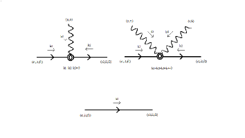
Figure 1: The figure illustrates the diagram associated to the new quark gluon interaction vertices. The analytic expression of the three legs vertex is given in (37) and the four legs one is defined by (38).

V One loop gluon self-energy evaluation

As it was mentioned before in connection with the extension of the work, the most important next step seems to consider the renormalization properties of the proposed modified version of QCD. This issue needs a separate study to be done.  However, let us consider here  two evaluations that can be simply made finite in the Minimal Substraction scheme (MS), but without adopting yet definitive renormalization conditions in order to not disregard important elements not yet clarified.

Specifically, we will evaluate the  one gluon self energy in the second order in the color coupling and all orders in the quark condensate parameters  $C_{f}=\frac{(2\pi)^{D}}{m_{f}}$ .   The close related two loops contribution to the vacuum energy in the same approximation, will be also calculated. In what follows the presented results correspond with calculations using the Feynman rules of reference muta for gluons and ghosts propagators and all the standard vertices of massless QCD, after complemented with the before defined rules for the new quark propagator and vertices.

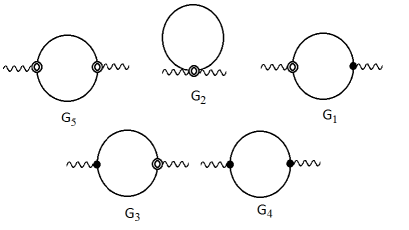
Figure 2: The picture shows the five diagrams associated to the fermion contribution to the two loop gluon self-energy. They are evaluated in the text in the same order as they appear from left to right in the figure.

The diagrams associated to the mentioned approximation for the self energy and in which the quarks participate are illustrated in figure 2.  The terms in which only gluons and ghost propagators and vertices enter are identical to the ones evaluated in Ref. muta are not needed to the evaluated. In the one loop approximation under consideration the diagrams entering are sums of  analytically identical terms for each of the flavours. Therefore, we will evaluate the contribution to the selfenergy given by only one flavour. The total contribution is the sum of the same expression obtained for one quark evaluated in the flavour couplings of each of the quark types. The expressions for all the appearing vertices and propagators associated to gluons and ghosts can be found in the exactly the same conventions used here in Ref. muta .  As an example, the wavy lines design the gluon propagator as given by.

$$D_{\mu\nu}^{ab}(k) =\frac{\delta^{ab}d_{\mu\nu}(k)}{k^{2}+i\epsilon},$$

$$d_{\mu\nu}(k) =g_{\mu\nu}-(1-\alpha)\frac{k_{\mu}k_{\nu}}{k^{2}},$$ (39)

and the vertices showing filled dots are the standard quark gluon, ghost gluon and the two types of gluon vertices as defined in Ref.  muta . The two kinds of vertices determined by the new terms in the action are represented by two concentric open circles.  In order to evaluate the polarization operator it is convenient to decompose this quantity in its transversal and longitudinal parts as follows

$$\Pi_{\mu\nu}^{ab}(k) =\Pi_{T}^{ab}(k)(g_{\mu\nu}-\frac{k_{\mu}k_{\nu}}{k^{2}})+\Pi_{L}^{ab}(k)\frac{k_{\mu}k_{\nu}}{k^{2}},$$ (40)

$$\Pi_{T}^{ab}(k) =\frac{1}{D-1}(g^{\mu\nu}-\frac{k^{\mu}k^{\nu}}{k^{2}})\Pi_{\mu\nu}^{ab}(k),$$ (41)

$$\Pi_{L}^{ab}(k) =\frac{k^{\mu}k^{\nu}}{k^{2}}\Pi_{\mu\nu}^{ab}(k).$$ (42)

It can be recalled that the fermion propagator (34) is the sum of one term being proportional to the spinor identity matrix and another one which is linear in the Dirac matrices. Also the new vertices both have a quadratic in the Dirac matrices structure. Therefore, it follows that the expression associated to the diagram  $G_{5}$ in figure (2), showing two of the new three legs vertices, decomposes in the sum of two expressions: one in which both propagators are of the ”$scalar$” type and another in which both are of the ”$fermion$” kind.  The same happens for the diagram $G_{4}$ in which two usual three legs vertices participate.   The terms associated to $G_{1}$ in which one of each of the new three legs vertex appears results in two times the expression in which one propagator is ”$scalar$” like  and the other one is of the ”$fermion$” type.

V.1 Diagram G₅

V.1.1 Scalar like propagators contribution $\Pi_{5\mu\nu}^{(s)ab}$

The analytic expression for graph $G_{5}^{(1)},$  in which both quark propagators are of the ”$scalar"$ type, after evaluating the color and spinor traces can be written in the form

$$\Pi_{5\mu\nu}^{(s)ab}(k)=-8g^{2}\delta^{ab}\int\frac{dp^{D}}{(2\pi)^{D}i}\frac{p_{\mu}p_{\nu}-q_{\mu}q_{\mu}+q^{2}g_{\mu\nu}}{(m_{f}^{2}-(p-\frac{q}{2})^{2})(m_{f}^{2}-(p+\frac{q}{2})^{2})}.$$ (43)

which determines the transversal and longitudinal parts as

$$\Pi_{5T}^{(s)ab}(k) =-2\frac{g^{2}\delta^{ab}}{(D-1)}\int\frac{dp^{D}}{(2\pi)^{D}i}\frac{4(p^{2}-\frac{(p.q)^{2}}{q^{2}})+(D-1)q^{2}}{(m_{f}^{2}-(p-\frac{q}{2})^{2})(m_{f}^{2}-(p+\frac{q}{2})^{2})},$$ (44)

$$\Pi_{5L}^{(s)ab}(k) =-2g^{2}\delta^{ab}\frac{1}{q^{2}}\int\frac{dp^{D}}{(2\pi)^{D}i}\frac{4(p.q)^{2}}{(m_{f}^{2}-(p-\frac{q}{2})^{2})(m_{f}^{2}-(p+\frac{q}{2})^{2})}.$$ (45)

V.1.2 Fermion like propagators contribution $\Pi_{5\mu\nu}^{(f)ab}$

Writing the analytic expression and calculating the traces of the diagram  $G_{5}$ in which the quark lines are ”$fermion$” like results in the expression

$$\Pi_{5\mu\nu}^{(f)ab}(k)=-\frac{1}{2}g^{2}\delta^{ab}m_{f}^{2}\int\frac{dp^{D}}{(2\pi)^{D}i}\frac{(4p^{2}+q^{2})(4p_{\mu}p_{\nu}-q_{\mu}q_{\nu}+q^{2}g_{\mu\nu})-8(p.q)^{2}g_{\mu\nu}}{(p-\frac{q}{2})^{2}(p+\frac{q}{2})^{2}(m_{f}^{2}-(p-\frac{q}{2})^{2})(m_{f}^{2}-(p+\frac{q}{2})^{2})}.$$ (46)

In this case the integrals for the transversal and longitudinal functions become

$$\Pi_{5T}^{(f)ab}(k) =-\frac{1}{2}\frac{g^{2}\delta^{ab}}{(D-1)}\int\frac{dp^{D}}{(2\pi)^{D}i}\frac{(4p^{2}+q^{2})(4(p^{2}-\frac{(p.q)^{2}}{q^{2}})+q^{2}(D-1))-8(p.q)^{2}(D-1)}{(p-\frac{q}{2})^{2}(p+\frac{q}{2})^{2}(m_{f}^{2}-(p-\frac{q}{2})^{2})(m_{f}^{2}-(p+\frac{q}{2})^{2})},$$ (47)

$$\Pi_{5L}^{(f)ab}(k) =-\frac{1}{2}g^{2}\delta^{ab}\frac{m_{f}^{2}}{q^{2}}\int\frac{dp^{D}}{(2\pi)^{D}i}\frac{4(4p^{2}-q^{2})(p.q)^{2}}{(p-\frac{q}{2})^{2}(p+\frac{q}{2})^{2}(m_{f}^{2}-(p-\frac{q}{2})^{2})(m_{f}^{2}-(p+\frac{q}{2})^{2})}.$$ (48)

The above integrals which determine the contribution to the diagram G₅ to the gluon selfenergy, in general contain more momentum dependent factors in the denominators that the ones in massless QCD at the same one loop level. However, those integrals, and the ones appearing in the rest of the contributions to the self-energy, can be systematically reduced to linear combinations of one loop scalar integrals, by employing the following definitions for the factors in the denominator determining the poles of the integrands

$$D_{1} =(p-\frac{q}{2})^{2},\text{ }D_{2}=(p+\frac{q}{2})^{2},$$

$$D_{3} =(m_{f}^{2}-(p-\frac{q}{2})^{2}),\text{ }D_{4}=(m_{f}^{2}-(p+\frac{q}{2})^{2}).$$ (49)

These relations can be inverted to express the quantities $p^{2}$ and $p.q$ in the numerators as linear functions of $q^{2}$ and the $D$ terms in various ways as follows

$$p^{2} =m_{f}^{2}-\frac{q^{2}}{4}-\frac{1}{2}(D_{3}+D_{4}),\text{ \ \ \ }p.q=\frac{1}{2}(D_{3}-D_{4}),$$

$$p^{2} =\frac{m_{f}^{2}}{2}-\frac{q^{2}}{4}-\frac{1}{2}(D_{4}-D_{1}),\text{ \ \ }p.q=\frac{m_{f}^{2}}{2}-\frac{1}{2}(D_{1}+D_{4}),$$

$$p^{2} =\frac{m_{f}^{2}}{2}-\frac{q^{2}}{4}-\frac{1}{2}(D_{3}-D_{2}),\text{ \ \ \ \ }p.q=-\frac{m_{f}^{2}}{2}+\frac{1}{2}(D_{2}+D_{3}),$$

$$p^{2} =-\frac{q^{2}}{4}+\frac{1}{2}(D_{1}+D_{2}),\text{ \ \ \ \ \ \ \ \ \ \ \ \ }p.q=\frac{1}{2}(D_{2}-D_{1}).$$ (50)

Then, the following identity  makes the work of decomposing the above Feynman integrals in simpler ones

$$\frac{m_{f}^{4}}{(p-\frac{q}{2})^{2}(p+\frac{q}{2})^{2}(m_{f}^{2}-(p-\frac{q}{2})^{2})(m_{f}^{2}-(p+\frac{q}{2})^{2})}$$

$$=\frac{m_{f}^{4}}{D_{1}D_{2}D_{3}D_{4}}$$

$$=\frac{1}{D_{1}D_{2}}+\frac{1}{D_{3}D_{4}}+\frac{1}{D_{1}D_{4}}+\frac{1}{D_{2}D_{3}}.$$ (51)

Since all  the integrands in the transversal and longitudinal parts are functions of  $p^{2}$ and $p.q$,  all of them can be expressed as functions of the $D$ factors and the square of the external momentum $q$, The following relations between the basic integrals  resulting in the various evaluations done here follow

$$0 =\int\frac{dp^{D}}{(2\pi)^{D}i}\frac{1}{D_{2}}=\int\frac{dp^{D}}{(2\pi)^{D}i}\frac{1}{D_{2}},$$

$$L_{m}(m_{f}) =\int\frac{dp^{D}}{(2\pi)^{D}i}\frac{1}{D_{3}}=\int\frac{dp^{D}}{(2\pi)^{D}i}\frac{1}{D_{3}},$$ (52)

$$\int\frac{dp^{D}}{(2\pi)^{D}i}\frac{D_{1}}{D_{3}} =\int\frac{dp^{D}}{(2\pi)^{D}i}\frac{D_{2}}{D_{4}}=m_{f}^{2}L_{m}(m_{f}),$$

$$\int\frac{dp^{D}}{(2\pi)^{D}i}\frac{D_{2}}{D_{3}} =\int\frac{dp^{D}}{(2\pi)^{D}i}\frac{D_{1}}{D_{4}}=(m_{f}^{2}+q^{2})L_{m}(m_{f}),$$

$$\int\frac{dp^{D}}{(2\pi)^{D}i}\frac{D_{3}}{D_{4}} =\int\frac{dp^{D}}{(2\pi)^{D}i}\frac{D_{4}}{D_{3}}=-q^{2}L_{m}(m_{f}),$$

$$\int\frac{dp^{D}}{(2\pi)^{D}i}\frac{D_{3}^{2}}{D_{4}} =\int\frac{dp^{D}}{(2\pi)^{D}i}\frac{D_{4}^{2}}{D_{3}}=((q^{2})^{2}+4\frac{m_{f}^{2}q^{2}}{D})L_{m}(m_{f}),$$

$$\int\frac{dp^{D}}{(2\pi)^{D}i}\frac{D_{1}^{2}}{D_{4}} =\int\frac{dp^{D}}{(2\pi)^{D}i}\frac{D_{2}^{2}}{D_{3}}=((m_{f}^{2}+q^{2})^{2}+4\frac{m_{f}^{2}q^{2}}{D})L_{m}(m_{f}).$$

Employing the results in references muta ; schroder ; smirnov , performing the Wick rotation and analytically integrating the appearing Feynman parametric integrals  with the use of the Wolfram Mathematica code,  the three basic integrals appearing in the above formulae can be evaluated.  The tadpole integral  has the form muta ; schroder

$$L_{m}(m_{f})=\int\frac{dp^{D}}{(2\pi)^{D}i}\frac{1}{(m_{f}^{2}+(p-\frac{q}{2})^{2})}=\frac{m_{f}^{D-2}}{(4\pi)^{\frac{D}{2}}}\Gamma(1-\frac{D}{2}).$$ (53)

The massive scalar self-energy  after making use of the formulae in Ref. muta , performing the Wick rotation and again analytically integrating the appearing Feynman parametric integral can be written as follows

$$L_{34}(q,m_{f}) =\int\frac{dp}{(2\pi)^{D}}\frac{1}{(m_{f}^{2}+(p-\frac{q}{2})^{2})((m_{f}^{2}+(p+\frac{q}{2})^{2})}$$

$$=\frac{1}{(4\pi)^{\frac{D}{2}}}\Gamma(2-\frac{D}{2})m_{f}^{\frac{D}{2}-2}\int_{0}^{1}dx(1+x(1-x)\frac{q^{2}}{m_{f}^{2}})^{\frac{D}{2}-2}$$

$$=\frac{\Gamma(\epsilon)}{(4\pi)^{2-\epsilon}}(\frac{m_{f}^{2}}{4m_{f}^{2}+q^{2}})^{\epsilon}\frac{\sqrt{4m_{f}^{2}+q^{2}}}{q}\times$$

$$(B[\frac{1}{2}(1+\frac{q}{\sqrt{4m_{f}^{2}+q^{2}}}),1-\epsilon,1-\epsilon]-$$

$$B[\frac{1}{2}(1-\frac{q}{\sqrt{4m_{f}^{2}+q^{2}}}),1-\epsilon,1-\epsilon]),$$ (54)

where $B[z,a,b]$  is the  Incomplete Gamma Function and as usual $\epsilon=2-\frac{D}{2}.$

$$B[z,a,b]=\int_{0}^{z}dtt^{a-1}(1-t)^{b-1}.$$ (55)

Next, the self-energy term including  one massive and one massless scalar, was also evaluated by employing the formula given in Ref. smirnov by after  the Wick rotation, analytically integrating the appearing parametric integral.    The result becomes

$$L_{14}(q,m_{f}) =\int\frac{dp}{(2\pi)^{D}i}\frac{1}{(p-\frac{q}{2})^{2}(m_{f}^{2}-(p+\frac{q}{2})^{2})}$$

$$=-\frac{\pi^{2-\epsilon}}{(4\pi)^{4-2\epsilon}}\Gamma(\epsilon)m_{f}^{-2\epsilon}\int_{0}^{1}dx\text{ }x^{-\epsilon}(1-(1-x)\frac{q^{2}}{m_{f}^{2}}-i\delta)^{-\epsilon}$$

$$=-\frac{\pi^{2-\epsilon}}{(4\pi)^{4-2\epsilon}}\frac{\Gamma(\epsilon)\Gamma(1-\epsilon)}{\Gamma(2-\epsilon)}(m_{f}^{2}+q^{2})^{-2\epsilon}\text{ }_{2}F_{1}(1-\epsilon,\epsilon,2-\epsilon,-\frac{q^{2}}{m_{f}^{2}-q^{2}}),$$ (56)

in which ${}_{2}F_{1}(a,b,c,z)$ is the Hypergeometric Function

$${}_{2}F_{1}(a,b,c,z)=\sum_{k=0}^{\infty}\frac{(a)_{k}(b)_{k}}{(c)_{k}}\frac{z^{k}}{k!},\text{ }(a)_{k}=\frac{\Gamma(a+k)}{\Gamma(a)}.$$ (57)

The  massless scalar self-energy integral results in

$$L_{12}(q) =\int\frac{dp}{(2\pi)^{D}i}\frac{1}{(p-\frac{q}{2})^{2}(p+\frac{q}{2})^{2}}$$

$$=-2^{4\epsilon-5}\pi^{\epsilon-\frac{3}{2}}(q^{2})^{-\epsilon}\frac{\Gamma(1-\epsilon)\Gamma(\epsilon)}{\Gamma(\frac{3}{2}-\epsilon)}.$$ (58)

Finally, the various contributions to the polarization operator associated to the diagram G₅, for each type of quark flavour $f$, can be written as explicit functions of the quark masses $m_{f}$ (or the quark condensate parameter $C_{f}$) and the space time dimension $D$ as follows. The amplitudes of the transversal components result in the form

$$\Pi_{5T}^{(s)ab}(q) =-4\frac{g^{2}\delta^{ab}m_{f}^{2}}{(D-1)}\left[(4m_{f}^{2}+(D-2)q^{2})L_{34}(q,m_{f})-2L_{m}(m_{f})\right],$$ (59)

$$\Pi_{5L}^{(s)ab}(q) =4g^{2}\delta^{ab}m_{f}^{2}L_{m}(m_{f}),$$ (60)

$$\Pi_{5T}^{(f)ab}(q) =T_{12}^{ab}(q)+T_{34}^{ab}(q)+T_{14}^{ab}(q)+T_{23}^{ab}(q),$$ (61)

$$T_{12}^{ab}(q) =0,$$ (62)

$$T_{34}^{ab}(q) =-\frac{g^{2}\delta^{ab}}{2(D-1)}\left(8(\frac{2}{D}-5)\text{ }L_{m}(m_{f})+4(4m_{f}^{2}+(D-2)q^{2})L_{34}(q,m_{f})\right),$$ (63)

$$T_{14}^{ab}(q) =T_{23}^{ab}(q)=-\frac{g^{2}\delta^{ab}}{2(D-1)}{\Large[(}2m_{f}^{2}(3-D)-2\frac{m_{f}^{4}}{q^{2}}+2q^{2}(D-2){\Large)}L_{14}(q,m_{f})+$$ (64)

$${\LARGE(}(1{\Large+}\frac{q^{2}}{m_{f}^{2}})(6-2D+2\frac{m_{f}^{2}}{q^{2}})+4(D+1)+2\frac{m_{f}^{2}}{q^{2}}+2(D-2)\frac{q^{2}}{m_{f}^{2}}$$

$$-\frac{2}{q^{2}}(m_{f}^{2}+2(1+\frac{2}{D})q^{2}+\frac{(q^{2})^{2}}{m_{f}^{2}}{\LARGE)}L_{m}(m_{f}){\Large]},$$

where the indices $(1,2),(3,4),(1,4)$ and ($2,3)$ here and below will indicate the contributions associated to the corresponding four terms in the decomposition (51) of the factor $\frac{1}{D_{1}D_{2},D_{3}D_{4}}$.

The longitudinal components get the expressions

$$\Pi_{5L}^{(f)ab}(k) =U_{12}^{ab}(q)+U_{34}^{ab}(q)+U_{14}^{ab}(q)+U_{23}^{ab}(q),$$ (65)

$$U_{12}^{ab}(q) =0,$$ (66)

$$U_{34}^{ab}(q) =g^{2}\delta^{ab}4(1+\frac{2}{D})\text{ }L_{m}(m_{f}),$$ (67)

$$U_{14}^{ab}(q) =U_{23}^{ab}(q)=-2g^{2}\delta^{ab}{\Large[(}\frac{m_{f}^{2}}{2q^{2}}(m_{f}^{2}-q^{2}{\Large)}L_{14}(q,m_{f})+$$ (68)

$${\LARGE(-}\frac{m_{f}^{2}}{2q^{2}}+(1+\frac{2}{D}){\LARGE)}L_{m}(m_{f}){\Large]}.$$

V.2 Diagram G₂    

This is the simplest of the calculations. After writing the analytic expression of the graph by following the Feynman rules and evaluating the color and spinor traces,  the polarization operator contribution becomes

$$\Pi_{2\mu\nu}^{ab}(q) =-4g^{2}\delta^{ab}g^{\mu\nu}\int\frac{dp^{D}}{(2\pi)^{D}i}\frac{1}{m_{f}^{2}-p^{2}}$$

$$=-4g^{2}\delta^{ab}L_{m}(m_{f})g^{\mu\nu},$$ (69)

$$\Pi_{2T}^{ab}(q) =\Pi_{2L}^{ab}(k)=-4g^{2}\delta^{ab}L_{m}(m_{f}),$$ (70)

in which the transversal and longitudinal parts becomes equal and proportional to the scalar massive tadpole integral.

V.3 Diagram G₁    

In this case, as noted before, since there is one new three legs vertex in the diagram, in which a product of two Dirac gamma matrices enter and another of the usual massless QCD which only contains one, the calculation reduces to two times the one in which one fermion like propagator and one scalar of the scalar type are employed in the internal lines.  Following the same steps as before, the integral giving the self-energy contribution associated to the quark flavour $f$ takes the form

$$\Pi_{1\mu\nu}^{ab}(k)=2g^{2}\delta^{ab}m_{f}^{2}\int\frac{dp^{D}}{(2\pi)^{D}i}\frac{(4p_{\mu}p_{\nu}-q_{\mu}q_{\mu}+(q^{2}+2p.q)g_{\mu\nu})}{(p+\frac{q}{2})^{2}(m_{f}^{2}-(p-\frac{q}{2})^{2})(m_{f}^{2}-(p+\frac{q}{2})^{2})}.$$ (71)

After getting from it the transversal part  and expressing the integrand in terms of the $D$ functions and $q^{2}$, allow to obtain the analytic expression of this transversal part in terms of the above given scalar integrals in the form written below

$$\Pi_{1T}^{ab}(q) =(W_{12}^{ab}(q)+W_{34}^{ab}(q)+W_{14}^{ab}(q)+W_{23}^{ab}(q)),$$ (72)

$$W_{12}^{ab}(q) =0,$$ (73)

$$W_{34}^{ab}(q) =\frac{g^{2}\delta^{ab}}{(D-1)}\left((D-2)\text{ }q^{2}+4m_{f}^{2})L_{34}(q,m_{f})+(\frac{4}{D}-6)\text{ }L_{m}(m_{f})\right),$$ (74)

$$W_{14}^{ab}(q) =\frac{8g^{2}\delta^{ab}}{D}L_{m}(m_{f}),$$ (75)

$$W_{23}^{ab}(q) =\frac{2g^{2}\delta^{ab}}{(D-1)}{\Large[(}m_{f}^{2}(3-D)+q^{2}(D-2)-\frac{m_{f}^{4}}{q^{2}}{\Large)}L_{14}(q,m_{f})+$$ (76)

$$\frac{(Dq^{2}+m_{f}^{2})}{q^{2}}L_{m}(m_{f}){\Large].}$$

Following the same steps as before, the evaluated expression for the coefficient of the longitudinal component becomes

$$\Pi_{1L}^{ab}(q) =-(X_{12}^{ab}(q)+X_{34}^{ab}(q)+X_{14}^{ab}(q)+X_{23}^{ab}(q)),$$ (77)

$$X_{12}^{ab}(q) =0,$$ (78)

$$X_{34}^{ab}(q) =4g^{2}\delta^{ab}(1+\frac{2}{D})\text{ }L_{m}(m_{f}),$$ (79)

$$X_{14}^{ab}(q) =-\frac{8g^{2}\delta^{ab}}{D}L_{m}(m_{f}),$$ (80)

$$X_{23}^{ab}(q) =-2g^{2}\delta^{ab}{\Large[}\frac{m_{f}^{2}}{q^{2}}{\Large(}m_{f}^{2}-q^{2})L_{14}(q,m_{f})+(2-\frac{m_{f}^{2}}{q^{2}})L_{m}(m_{f}){\Large].}$$ (81)

The contribution of the diagram $G_{3}$ exactly coincides with the just evaluated for $G_{1}.$ This can be seen by performing a mood change of the

momentum integration variable in the expression for G₁.

V.4 Diagram G₄

The process of evaluation of the diagram $G_{4}$ follows the same steps as the ones for $G_{5}.$  The form of the results for the integral after the traces are calculated is

$$\Pi_{4\mu\nu}^{ab}(k) =\Pi_{1\mu\nu}^{(A)ab}(k)+\Pi_{1\mu\nu}^{(B)ab}(k),$$ (82)

$$\Pi_{4\mu\nu}^{(A)ab}(k) =-2g^{2}\delta^{ab}m_{f}^{2}g_{\mu\nu}\int\frac{dp^{D}}{(2\pi)^{D}i}\frac{1}{(m_{f}^{2}-(p-\frac{q}{2})^{2})(m_{f}^{2}-(p+\frac{q}{2})^{2})}$$ (83)

$$=-2g^{2}\delta^{ab}m_{f}^{2}L_{34}(q,m_{f})g_{\mu\nu},$$

$$\Pi_{4\mu\nu}^{(B)ab}(k) =-g^{2}\frac{\delta^{ab}m_{f}^{4}}{2}\int\frac{dp^{D}}{(2\pi)^{D}i}\frac{8p_{\mu}p_{\nu}-2q_{\mu}q_{\mu}+(q^{2}-4p^{2})g_{\mu\nu}}{(p-\frac{q}{2})^{2}(p+\frac{q}{2})^{2}(m_{f}^{2}-(p-\frac{q}{2})^{2})(m_{f}^{2}-(p+\frac{q}{2})^{2})},$$ (84)

and the explicit formulae for the coefficients of the transversal and longitudinal parts of $\Pi_{4\mu\nu}^{(A)ab}$ are

$$\Pi_{4T}^{(A)ab}(k)=\Pi_{4L}^{(A)ab}(k)=-2g^{2}\delta^{ab}m_{f}^{2}L_{34}(q,m_{f}).$$ (85)

Similarly, the result for the transversal part of the contribution $\Pi_{1\mu\nu}^{(B)ab}$ in terms of the basic integrals become

$$\Pi_{4T}^{ab}(q) =B_{12}^{ab}(q)+B_{34}^{ab}(q)+B_{14}^{ab}(q)+B_{23}^{ab}(q),$$ (86)

$$B_{12}^{ab}(q) =-\frac{g^{2}(D-2)}{(D-1)}\delta^{ab}q^{2}L_{12}(q,m_{f}),$$ (87)

$$B_{34}^{ab}(q) =-\frac{g^{2}\delta^{ab}}{(D-1)}\left(2(D-2)\text{ }L_{m}(m_{f})+(2m_{f}^{2}(3-D)+2q^{2}(D-2))L_{34}(q,m_{f})\right),$$ (88)

$$B_{14}^{ab}(q) =B_{23}^{ab}(q)=-\frac{g^{2}\delta^{ab}}{2(D-1)}{\Large[(}2(2-D)+2\frac{m_{f}^{2}}{q^{2}}{\Large)}L_{m}(m_{f})+{\Large(}m_{f}^{2}(3-D)+2q^{2}(D-2)-\frac{2m_{f}^{4}}{q^{2}}{\Large)}L_{14}(q,m_{f}){\Large].}$$ (89)

Finally, the longitudinal term get the expression

$$\Pi_{4L}^{ab}(q) =C_{12}^{ab}(q)+C_{34}^{ab}(q)+C_{14}^{ab}(q)+C_{23}^{ab}(q),$$ (90)

$$C_{12}^{ab}(q) =0,$$ (91)

$$C_{34}^{ab}(q) =2g^{2}\delta^{ab}m_{f}^{2}\text{ }L_{34}(q,m_{f}),$$ (92)

$$C_{14}^{ab}(q) =C_{23}^{ab}(q)=-g^{2}\delta^{ab}m_{f}^{2}{\Large(}\frac{m_{f}^{2}}{q^{2}}-1)L_{14}(q,m_{f})+g^{2}\delta^{ab}\frac{m_{f}^{2}}{q^{2}}L_{m}(m_{f}){\Large].}$$ (93)

V.5 Gauge invariance and total transversal polarization operator

After adding all the above evaluated contributions to the longitudinal component of the selfenergy it follows

$$\Pi_{L}^{ab}(q) =\Pi_{5L}^{ab}(q)+\Pi_{2L}^{ab}(q)+\Pi_{1L}^{ab}(q)+\Pi_{3L}^{ab}(q)+\Pi_{4L}^{ab}(q)$$

$$=0.$$ (94)

Therefore, the transversality property is satisfied by the self-energy as it should be since it is a Ward identity which must be satisfied by any correction to the self-energy given by a well defined order in the perturbation theory.  Since, here we evaluated all the terms in the expansion which are of order two in the strong coupling being and exact (to all orders )  in the flavour condensate parameters, the transversality should be satisfied.

Further, after also adding all the  transversal contributions and simplifying the result, the total unrenormalized one loop gluon self-energy can be written in the form

$$\Pi_{\mu\nu}^{ab}(q) =\Pi_{T}^{ab}(q)(g_{\mu\nu}-\frac{q_{\mu}q_{\nu}}{q^{2}}),$$ (95)

$$\Pi_{T}^{ab}(q) =\Pi_{5T}^{ab}(q)+\Pi_{2T}^{ab}(q)+\Pi_{1T}^{ab}(q)+\Pi_{3T}^{ab}(q)+\Pi_{4T}^{ab}(q)$$ (96)

$$=-\frac{g^{2}\delta^{ab}}{D(D-1)}(D(D-26)+8)L_{m}(m_{f})+\frac{g^{2}\delta^{ab}(2-D)}{(D-1)}q^{2}L_{12}(q)+$$

$$+\frac{g^{2}\delta^{ab}}{2(D-1)}(-2D(D+17)m_{f}^{2}-9D(2+D)q^{2})L_{34}(q,m_{f}).$$

Employing the  Minimal Substraction renormalization scheme (MS),  the one loop divergences can be eliminated by deleting the terms showing poles in the expansion of the above expression in a Laurent series in the parameter $\epsilon=\frac{4-D}{2}.$ However, the resulting expression is cumbersome and since we will not analyze it here, is not written. After adding to $\Pi_{T}^{ab}(q)$ the free part of the gluon equation of motion, the  following expressions for the gluon one loop propagator and its inverse follow

$$D_{\mu\nu}^{ab-1}(q) =\delta^{ab}q^{2}(g_{\mu\nu}-(1-\alpha)\frac{q_{\mu}q_{\nu}}{q^{2}})-\Pi_{T}^{ab}(q)(g_{\mu\nu}-\frac{q_{\mu}q_{\nu}}{q^{2}})$$ (97)

$$=(q^{2}-\Pi_{T}^{ab}(q))(g_{\mu\nu}-\frac{q_{\mu}q_{\nu}}{q^{2}})+\alpha\frac{q_{\mu}q_{\nu}}{q^{2}},$$

$$\Pi_{T}^{ab}(q) =\delta^{ab}\Pi_{T}(q),$$ (98)

$$D_{\mu\nu}^{ab}(q) =\frac{\delta^{ab}}{(q^{2}-\Pi_{T}(q))}(g_{\mu\nu}-\frac{q_{\mu}q_{\nu}}{q^{2}})+\frac{\delta^{ab}}{\alpha}\frac{q_{\mu}q_{\nu}}{q^{2}}.$$ (99)

VI Vacuum energy

Let us consider below the main steps in the evaluation of the one and two loops corrections to the effective action which will give the negative of the vacuum energy as a function of the quark masses  $m_{f}$ in that approximation.

VI.1 One loop term

The one loop term reduces to the logarithm of the determinant of the new form of the inverse quark propagator, which is the result of the functional integral defining free quark generating functional.  The calculation of this term, following usual steps in this special case, is sketched below

$$\Gamma^{(2)}(m_{f}) =\frac{1}{i}\sum_{p}\log\det G^{-1}(p)$$

$$=-V^{D}\sum_{p}\frac{dp^{D}}{(2\pi)^{D}i}\log\det G(p)$$

$$=-V^{D}\sum_{p}\frac{dp^{D}}{(2\pi)^{D}i}\log\det[\frac{m_{f}}{m_{f}^{2}-p^{2}}(1-m_{f}\frac{\gamma_{\mu}p^{\mu}}{p^{2}})]$$

$$=-V^{D}\sum_{p}\frac{dp^{D}}{(2\pi)^{D}i}\log\det[\frac{m_{f}}{m_{f}^{2}-p^{2}}I]-\frac{V^{D}}{2}\sum_{p}\frac{dp^{D}}{(2\pi)^{D}i}\log\det[\frac{p^{2}-m_{f}^{2}}{p^{2}}I]$$

$$=V^{D}\sum_{p}\frac{dp^{D}}{(2\pi)^{D}i}2N\text{ }\log[m_{f}^{2}-p^{2}]+V^{D}\sum_{p}\frac{dp^{D}}{(2\pi)^{D}i}2N\text{ }\log[\frac{p^{2}}{m^{2}}].$$ (100)

After taking the derivative the expression over $m_{f}^{2}$, it follows

$$\frac{d}{dm_{f}^{2}}\Gamma^{(0)}(m_{f}) =V^{D}2N\int\frac{dq^{D}}{(2\pi)^{D}i}\frac{1}{m_{f}^{2}-p^{2}}$$

$$=V^{D}2N\text{ }L_{m}(m_{f})$$

$$=V^{D}2N\text{ }\frac{\Gamma(1-\frac{D}{2})m_{f}^{D-2}}{(4\pi)^{\frac{D}{2}}},$$ (101)

which when integrated over $m_{f}^{2}$ in the interval $(0,m_{f}^{2})$ by assuming $\epsilon$ being in a region in which its real part is negative, leads to

$$\Gamma^{(0)}(m_{f})=V^{D}2N\text{ }\frac{\Gamma(\epsilon-1)(m_{f}^{2})^{2-\epsilon}}{(4\pi)^{\frac{D}{2}}(2-\epsilon)}.$$ (102)

The finite part of the above expression in the Laurent series expansion can be evaluated by employing the expression of $V^{D}$ in terms of the four-dimensional volume and the dimensional regularization scale parameter $\mu$

$$V^{D}=\mu^{4-D}V^{4}=\mu^{2\epsilon}V^{4}.$$ (103)

Then, the finite part the one loop effective action in the MS scheme becomes

$$\Gamma_{fin}^{(0)}(m_{f}) =2N\frac{m_{f}^{4}}{(4\pi)^{2}}\log(\frac{m_{f}}{\mu})-\frac{m_{f}^{4}}{(4\pi)^{2}}(3-\gamma+\log(4\pi))$$

$$=-V_{fin}^{(0)}(m_{f}).$$ (104)

The result after changed its sign, gives the dependence on $m_{f}$ of the vacuum energy in this approximation. The potential decreases at large mass values indicating the dynamical generation of the mass in this approximation. This outcome for the first correction was also obtained in Refs. epjc2 ; epjc19 ; ana ,

VI.2 Two loop terms

The two loop vacuum energy can be readily evaluated starting from the already known transversal part.  This follows, thanks to the formula

$$\Gamma^{(2)}(m_{f}) =\frac{(D-1)}{2}\int\frac{dq^{D}}{(2\pi)^{D}i}\frac{\Pi_{T}^{aa}(q)}{q^{2}}$$

$$=\frac{(D-1)(N^{2}-1)}{2}\int\frac{dq^{D}}{(2\pi)^{D}i}\frac{\Pi_{T}(q)}{q^{2}},$$ (105)

which follows after noting that the diagrams defining the two loop approximation for the effective action can be organized as the sum of the diagrams defining the self-energy contracted with the gluon free propagator.

After substituting in the above formula the evaluated expression for $\Pi_{T}$ it follows

$$\Gamma^{(2)}(m_{f}) =-\frac{g^{2}(N^{2}-1)}{2D}(D(D-26)+8)\int\frac{dq^{D}}{(2\pi)^{D}i}\frac{L_{m}(m_{f})}{q^{2}}+\frac{g^{2}\delta^{ab}(2-D)}{(D-1)}\int\frac{dq^{D}}{(2\pi)^{D}i}L_{12}(q)+$$

$$+\frac{g^{2}(N^{2}-1)}{4}\int\frac{dq^{D}}{(2\pi)^{D}i}(-\frac{2D(D+17)m_{f}^{2}}{q^{2}}+9D(2-D))L_{34}(q,m_{f}).$$ (106)

In the above formula, the first and the second terms vanish in dimensional regularization.   The third one can be expressed

as follows

$$\Gamma^{(2)}(m_{f}) =+\frac{g^{2}9(N^{2}-1)D(2-D)V^{D}}{4}\int\frac{dq^{D}}{(2\pi)^{D}i}\frac{dp^{D}}{(2\pi)^{D}i}\frac{1}{(m^{2}-q^{2})(m^{2}-p^{2})}$$

$$+\frac{g^{2}(N^{2}-1)D(D+17)m_{f}^{2}}{2}\int\frac{dq^{D}}{(2\pi)^{D}i}\frac{dp^{D}}{(2\pi)^{D}i}\frac{1}{q^{2}(m^{2}-q^{2})(m^{2}-(p-q)^{2})}.$$ (107)

Each of the two integrals appearing in the first term is equal to the  $L_{m}$ in (52).  The second term is proportional to a two loop scalar Master Integral

given in Ref. schroder . Then, the unrenormalized two loops effective action has the form

$$\Gamma^{(2)}(m_{f}) =+\frac{9(N^{2}-1)D(2-D)V^{D}}{4}\frac{\Gamma^{2}(1-\frac{D}{2})}{(4\pi)^{D}}m_{f}^{2D-4}g^{2}V^{D}$$

$$-\frac{(N^{2}-1)D(D+17)}{2}\frac{(D-2)\Gamma^{2}(2+\epsilon)\Gamma^{2}(1-\frac{D}{2})}{2^{2D+1}(D-3)}g^{2}m_{f}^{2D-4}V^{D}.$$ (108)

Substituting  the formulae for the coupling $g$ and the $D$ dimensional volume $V^{D}$according to

$$g=g_{0}\mu^{D},\text{ \ \ \ }V^{D}=\mu^{2\epsilon}V^{4},$$

it follows

$$g^{2}m_{f}^{2D-4}V^{D}=g_{0}^{2}V^{4}m_{f}^{4}m_{f}^{-4\epsilon}.$$

Afterwards, expanding the formula (108) in Laurent series around $\epsilon=0$, deleting the pole terms and tending to the limit $\epsilon\rightarrow 0$ leads to the finite value of the two loop contribution to the effective action in the MS scheme

$$\Gamma^{(2)}(m_{f}) =-273.18\text{ }\frac{g_{0}^{2}}{4\pi}m_{f}^{4}\text{ }+322.47\text{ }\frac{g_{0}^{2}}{4\pi}\text{ }m_{f}^{4}Log(\frac{m_{f}}{\mu})-$$ (109)

$$132.527\text{ }m_{f}^{4}\text{ }\frac{g_{0}^{2}}{4\pi}\text{ }Log^{2}(\frac{m_{f}}{\mu}).$$ (110)

The total effective potential is then given by the expression

$$V(m_{f}) =0.0656145\text{ }m_{f}^{4}\text{ }+273.18\text{ }m_{f}^{4}\text{ }\frac{g_{0}^{2}}{4\pi}-(0.0379954\ +$$ (111)

$$322.47\text{ }\frac{g_{0}^{2}}{4\pi})\text{ }m_{f}^{4}\text{ }Log(\frac{m_{f}}{\mu})+132.527\text{ }m_{f}^{4}\text{ }\frac{g_{0}^{2}}{4\pi}\text{ }Log^{2}(\frac{m_{f}}{\mu}).$$ (112)

In Figure 3 the potential divided by the fourth power of the renormalization parameter $\mu$ is plotted as a function of the mass divided by $\mu$ for various small values of the coupling constant $g_{0}$. For higher values the coupling minimum of the minimum of the potential tends to disappear. However, as it was remarked before, the two loop approximation is insufficient to define whether or not the scheme predicts a hierarchical flavour dynamic symmetry breaking.  Therefore, the evaluation done should not be expected to be relevant for answering the main physical question: the possibility of large quark mass generation at the values of the strong coupling.   However,  the results shown in Figure 3 indicate that at small values of the gauge coupling, the interaction is able to generate large masses for the fermions. The figure corresponds to fix as an example $\mu=1$   GeV , then it follows that for a  small coupling near the value $g_{0}=0.0271828$ the fermion mass gets a value near the top quark mass $m_{f}=173$  GeV.   This  evaluation suggests the interesting possibility that, if the theory is in fact equivalent to the massless one, the  generation of large mass mechanism could also work for the low coupling electroweak scale.

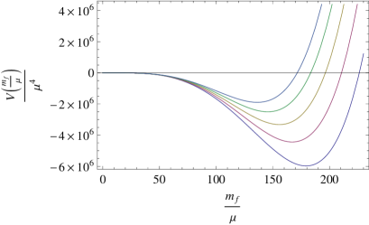
Figure 3: The figure illustrates the effective potential divided by $\mu^{4}$ as function of the ratio $\frac{m_{f}}{\mu}$. At $\mu=1$ GeV various small values of the coupling constant around $g_{0}=0.0271828$ were chosen to evidence that the minimum of the potential can be fixed at a $m_{f}$  being close to the top quark mass of $173$ GeV. For higher values of the coupling the minimum tends to disappear. However, as described in the text, the lack of the possibility for generating a hierarchy of mass in the considered two loops approximation, determines the need for improving the evaluation of the potential, in order to decide whether or not a large and hierarchical mass generation effect can be predicted at the large values of the strong coupling observed in Nature.

VII Summary

We have proposed an improved version of the modified version of QCD discussed in previous works, which shows local gauge invariance and include the same kind of gluon and fermion condensate parameters. The analysis done for constructing the proposal suggests its equivalence with massless QCD, after considered with a special renormalization procedure designed to implement the dimensional transmutation effect. In respect to the gluon condensation properties, the theory should reproduce the previous derivation of the constituent mass for the light quarks  given in epjc ; jhep and the Savvidy kind of potential as a function of the gluon condensate parameter. The study of the possible improvement in the predictions determined by the gained gauge invariance and locality of the description will be considered elsewhere. For the case of only retaining the fermion condensate parameter, the fermion auxiliary functions were integrated leading to a theory described by a new Lagrangian given by the massless QCD one but including a new gauge invariant term for each quark flavour. The new Lagrangian terms can be considered as local modifications of the ones derived in Ref. ana . In the same form, they have a similar component constituted by the product of two gluon and two quark fields, but now evaluated in the same space-time point.  The new terms also show components leading to three legs vertices which were absent in the previous form of the generating functional. The terms determines masses for all the six quarks which are given by the reciprocal of the new flavour condensate couplings linked with each quark type. Therefore, the strength of the condensate couplings decreases with the masses of the associated quarks. The gluon self-energy was evaluated up to the second order in the gauge coupling including all orders of the flavour condensate ones. The result, being associated to a well defined order in the couplings, satisfies the transversality condition as required by the gauge invariance. In addition, it is also gauge parameter independent. The transversal part of the self energy is employed to evaluate the two loop contribution to the effective action at zero mean fields (minus the vacuum energy) as a function of the flavour condensate couplings. The transversality and gauge parameter independence of the gluon self-energy, then also determined the gauge parameter independence of the evaluated potential. Afterwards, in order to interpret the result, we assumed that the introduced flavour couplings represent dynamically generated quantities, as it was effectively the case in the precedent works for the similar non gauge invariant couplings which motivated their consideration in this study. Then, in this first approximation, the potential is able to predict the dynamic generation of quark masses, for sufficiently small values of the QCD coupling. It can be remarked that the generation happening only for small couplings at the considered approximation, does not mean a negative answer to the question about whether or not the scheme can address the quark mass hierarchy. This is can be understood by noting that in the two loop order, the diagrams can not yet incorporate lines associated to two different kinds of flavours. For this appearance to happens, at least three loops corrections are required. It is reasonable that in order to explain the quark mass hierarchy as a dynamic flavour symmetry breaking, there should exist ”interference” like effects in the vacuum energy corrections. In them, the contributions of diagrams showing two or more kinds of fermion lines might tend to rise the energy of the configurations with equal values of the quark condensates, making them more energetic that the ones in which one of the quark condensate parameters gets a large value and the others hierarchical lower ones. At the moment we have the impression that the considered framework is ideal to realize the Democratic Symmetry Breaking properties of the mass hierarchy remarked in Refs. fritzsch ; fritzsch1 . The predictions of the general discussion including gluon condensates for the low energy processes, as well as the renormalization properties and the evaluation of three loop contributions in the case of only having the fermion condensate, are expected to be considered elsewhere.

References

• (1) Y. Nambu and G. Jona-Lasinio, Phys. Rev. 122, 345 (1961).
• (2) H. Fritzsch, Nucl. Phys. B155, 189 (1979).
• (3) H. P. Nilles, Phys. Lett. B 115, 193 (1982).
• (4) H. Fritzsch, Nucl. Phys. B (Proc. Suppl.) 40, 121 (1995).
• (5) W. A. Bardeen, C. T. Hill and M. Lindner, Phys. Rev. D41, 1647 (1990).
• (6) L. S. Celenza, Chueng-Ryong Ji and C. M. Shakin, Phys. Rev. D36, 895 (1987).
• (7) C. J. Burden, C. D. Roberts and A. G. Williams, Phys. Lett. B285, 347 (1992).
• (8) H.-P. Pavel, D. Blaschke and G. Ropke, Int. Jour. Mod. Phys. A14, 205 (1999).
• (9) M. A. Shifman, A. I. Vainshtein and V. I. Zakharov, Nucl. Phys. B147,  385, 448 (1979).
• (10) R. Fukuda, Phys. Rev. D21, 485 (1980).
• (11) S. Coleman and E. Weinberg, Phys. Rev. D7, 1888 (1973).
• (12) V.A. Miransky, in Nagoya Spring School on Dynamical Symmetry Breaking, ed. K. Yamawaki, World Scientific (1991).
• (13) H. Fritzsch and P. Minkowski, Phys. Rep. 73, 67 (1981).
• (14) D. E. Clague and G. G. Ross, Nucl. Phys. B364, 43 (1991).
• (15) A. Cabo, S. Peñaranda and R. Martínez, Mod. Phys. Lett. A10, 2413 (1995).
• (16) M. Rigol and A. Cabo, Phys. Rev. D62, 074018 (2000).
• (17) A. Cabo and M. Rigol, Eur. Phys. J. C23, 289 (2002).
• (18) A. Cabo and M. Rigol, Eur. Phys. J. C47, 95 (2006).
• (19) A. Cabo and D. Martinez-Pedrera, Eur. Phys. J. C47, 355 (2006).
• (20) A. Cabo, Eur. Phys. J. C55, 85 (2008).
• (21) A. Cabo, JHEP 04, 044 (2003).
• (22) A. Cabo, N. G. Cabo-Bizet and A. Cabo Bizet, Eur. Phys. J. C64, 133 (2009).
• (23) P. Hoyer, NORDITA-2002-19 HE (2002), e-Print Archive: hep-ph/0203236 (2002).
• (24) P. Hoyer, Proceedings of the ICHEP 367-369, Amsterdam (2002), e-Print Archive: hep-ph/0209318.
• (25) P. Hoyer, Acta Phys. Polon. B34, 3121 (2003). e-Print Archive: hep-ph/0304022.
• (26) N. Nakanishi and I. Ojima, Covariant Operator Formalism of Gauge Theories and Quantum Gravity, World Scientific, Singapore, (1990).
• (27) T. Muta, Foundations of Quantum Chromodynamics, World Scientific Lectures Notes in Physics, Vol. 5, (1987).
• (28) S. Gasiorowicz, Elementary Particle Physics Wiley, New York, (1966).
• (29) Y. Schröder and A. Vuorinen, JHEP 0506: 051, (2005).
• (30) V. A. Smirnov, Feynman Integral Calculus Srpinger Tracts in Modern Physcis Vol. 211, Ed. G. Höler, Springer-Verlag, Berlin Heidelberg (2006).