]http://www.randomlasers.com

Probing the dynamics of Anderson localization through spatial mapping

Abstract

We study (1+1)D transverse localization of electromagnetic radiation at microwave frequencies directly by two-dimensional spatial scans. Since the longitudinal direction can be mapped onto time, our experiments provide unique snapshots of the build-up of localized waves. The evolution of the wave functions is compared with numerical calculations. Dissipation is shown to have no effect on the occurrence of transverse localization. Oscillations of the wave functions are observed in space and explained in terms of a beating between the eigenstates.

Recent years witnessed a renaissance in experimental studies on Anderson localization. This phenomenon, conceived by P. W. Anderson in 1958 Anderson1958 , originally described the absence of diffusion of electrons in random lattices due to interference. Since Anderson localization is in essence a wave phenomenon, physicists have successfully extended the scope of localization studies to electromagnetic waves Anderson1985 ; John1987 ; Genack2000 ; Genack2011 , ultrasound vanTiggelen2008 , and matter waves Aspect2009 ; Inguscio2009 ; DeMarco2011 .

Similar to other phase transition phenomena, dimensionality plays an important role. For $d\leq 2$, all states are localized, whereas for $d=3$ a phase transition from diffusive to localized behavior occurs at a critical scattering strength GangOfFour1979 . In the special case of transverse localization, formulated by De Raedt et al. DeRaedt1989 , one dimension is designed not to be disordered, whereas disorder is introduced in the other dimension(s). As a consequence, waves spread out in the disorder-free dimension, but are confined in the other dimensions. Waves are always localized in the transverse directions as long as the transverse system length $L$ is larger than the localization length $\xi$. Effectively, transverse localization reduces the number of spatial coordinates in the system: the coordinate along which the sample is extruded can be seen as the time-axis in the time-dependent Schrödinger equation. Stationary transverse localization experiments could thus provide a unique insight into how a localized wave develops over time. Studying and understanding this intriguing aspect of transverse localization experimentally is the central topic of this paper.

Pivotal experiments on weakly scattering disordered photonic lattices Schwartz2007 ; Silverberg2008 ; Segev2011 have focussed on the observation of localized wave functions after a certain fixed propagation distance and the effect of nonlinearity on the transverse localization length. Both theoretical and experimental studies have revealed interesting dynamical properties of the periodically kicked quantum rotator which bears close resemblance to Anderson localization Prange1982 ; Raizen1995 , suggesting that studying the dynamics of localization itself is important. The unique property of transverse localization experiments that enables us to map one spatial dimension onto time is ideally suited for this purpose.

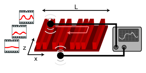
Figure 1: Experimental set-up. Nylon bars (red) are placed on top of an oxygen free copper plate, the distance between the bars is random in the transverse x-direction. The z-direction is disorder free. One of the two microwave antennas (black disks) is scanned over the sample and a vector network analyzer is used to measure the transmitted spectrum between the two antennas. Each scan along the x-axis is equivalent to a snapshot in time.

First, we provide new results on transverse localization by performing experiments with microwaves in 2D. Instead of measuring the intensity at the end of our samples, we study the evolution of the extent of the waves as a function of propagation distance. Second, we compare our experimental results with numerical solutions to a 2D Schrödinger-like equation from which we deduce information regarding the effect of dissipation on localization. Since localization was introduced for classical waves the issue of absorption has been the subject of immense discussions and various opinions Anderson1985 ; John1985 . Tackling this issue has shown to be unavoidable in any experiment Weaver1993 ; Beenakker1996 ; Wiersma1997 ; Maret1999 ; Genack2009 . To study both the dynamics of localized waves and the effect of unavoidable dissipation, we performed measurements on samples consisting of scattering bars placed parallel to each other in an open system. Such samples form an excellent model system in which out-of-plane scattering plays the role of dissipation, whereas propagation along the bars represents the dynamics. Interesting non-stationary behavior of single localized wave functions is observed, which we analyze by decomposing these functions into the system’s eigenstates semi-analytically.

Experimental methods - Figure 1 shows a sketch of the experimental apparatus. Samples were fabricated by placing nylon bars (3 mm $\times$ 10 mm $\times$ 1000 mm) on top of an oxygen free copper plate (500 mm $\times$ 1000 mm). These nylon bars ($n=1.73$ NylonHP ) are the scatterers in our system. Disorder was introduced into the system by varying the spacing between the nylon bars. The spacings were chosen randomly from a Poissonian distribution with a mean of 10 mm. Introducing Poissonian disorder makes sure that the presence of stop band effects is negligible Segev2011b . In addition, ordered samples were prepared with a lattice spacing of 20 mm in which clear stop bands were observed and calculated around 7 and 13 GHz. Styrofoam spacers ensured parallel alignment of the nylon bars. We studied the sample by measuring the microwave transmission spectrum with varying bandwidths around 10 GHz using a vector network analyzer (Rhode and Schwartz ZVA 67). The detection antenna was scanned over the sample by using a stepper motor (Newport ESP 301) and a home-built scanning stage.

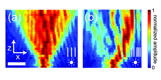
Figure 2: Experimentally determined false color images of the amplitude distribution for (a) an ordered and (b) a disordered sample at 9.2 GHz . Every row is normalized independently. The scale bar denotes 100 mm.

Results - The propagation of waves within an ordered and a disordered sample is shown in Fig. 2. The excitation frequency was set at 9.2 GHz, that is outside any of the stop gaps of the ordered sample. The data was normalized for every row in the xz-plane to enhance the visibility of the wave function far away from the source. In the ordered sample, Fig. 2(a), waves spread out ballistically as a function of propagation distance. However, for the disordered sample, Fig. 2(b), the wave propagation is strikingly different: the wave initially spreads out, but at a certain stage stays confined to a bounded region. These type of two-dimensional spatial scans provide us with exceptional data for analyzing transverse localization in unprecedented detail.

In order to quantify the transverse confinement of wave intensity as function of propagation distance, we calculate the inverse participation length (IPL) Mirlin1993 . The IPL for a one-dimensional intensity distribution $I(x)$ is defined as

$$P(z)\equiv\frac{\int I^{2}(x,z){\rm d}x}{\left(\int I(x,z){\rm d}x\right)^{2}}$$ (1)

and has a unit of inverse length. The IPL is inversely proportional to the spread of the wave function: a homogeneously extended wave spread out over the entire sample length $L$ leads to an IPL of $1/L$. To obtain a reliable value for the spread of wave functions, the ensemble averaged intensity profiles were determined by averaging over 20 realizations of disorder.

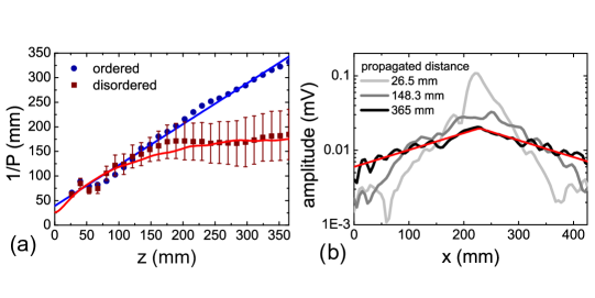
Figure 3: (a) Participation ratio versus propagation distance at 9.2 GHz for an ordered sample (blue) and a disordered ensemble (red). Red line: calculation for an ensemble of 100 disordered samples. Blue line: linear fit. (b) Transverse ensemble averaged amplitude distribution for different propagation distances. Red line: exponential fit.

Figure 3(a) shows how the inverse of the IPL develops with increasing propagation distance for both the ordered sample and the ensemble of disordered samples at 9.2 GHz. In agreement with the qualitative picture we obtained from Fig. 2, we see that the extent of the wave function given by the inverse of the IPL increases linearly for the ordered sample. For the disordered ensemble on the other hand the IPL flattens off after a certain propagation distance. This settling of the IPL to a finite value constitutes a direct experimental observation of the spatial evolution of transversely localized waves.

Besides a different evolution of the waves’ extent, the eventual spatial shape of the ensemble averaged wave function distinguishes localized from extended waves as well. In contrast to Gaussian shaped extended wave functions, localized wave functions obtain exponential tails. Figure 3(b) shows the ensemble averaged wave function profile for three different propagation distances on a semi-logarithmic scale. Close to the excitation source, the ensemble averaged wave function is strongly peaked in the transverse dimension. For longer propagation distances, the intensity in the wings of the wave function increases and the peak becomes less pronounced. The ensemble averaged wave function quenches once the localization length is reached and its shape is well described by an exponential. From an exponential fit to the data we find a localization length of 192 $\pm$ 6 mm.

After having studied these ensemble averaged properties of our system, we now aim to understand the propagation of waves for single realizations of disorder. In Fig. 4(a), we plot the spatial profile for 17 different excitation positions in one sample after 365 mm of propagation. Based on Fig. 3, this distance ensures we are truly looking at localized wave functions. The individually measured spatial profiles are strongly dependent on the position of the excitation antenna. To a large extent the detected radiation follows the position of the excitation antenna as indicated by the white diagonal. Naively, one might expect for a localizing sample clearly isolated regions of higher intensity that are independent on the position of excitation. Such patterns would appear as vertical stripes in Fig. 4(a). However, much to our surprise, the spatial patterns of these isolated regions along the transverse dimension $x$ are dependent on the excitation position. In fact, for the measurement shown in Fig. 4, some patterns appear to be anti-diagonal. Furthermore, the excitation map displays a high degree of symmetry along the diagonal.

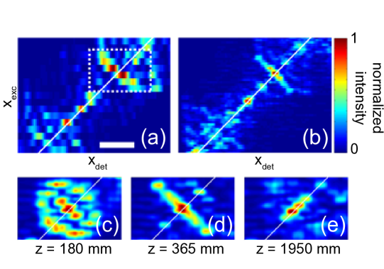
Figure 4: (a) Experimental and (b) numerically calculated false color plots of the wave function intensity in transverse direction after 365 mm of propagation along the z-direction for different positions of the excitation antenna at 9.2 GHz. The white lines indicate the position of the excitation antenna. The dashed box marks an anti-diagonal wave profile. Scale bar denotes 100 mm. (c-e) show calculations using mode decomposition for the area marked with the dashed box in (a) for 180, 365, and 1950 mm of propagation respectively. Beating of eigenmodes can result in (c) circular, (d) anti-diagonal, or (e) diagonal patterns.

Model - In order to build a basis for understanding the ensemble averaged data and the remarkable excitation dependence of localized wave functions in single realizations of disorder, the system is analyzed numerically and semi-analytically. In the paraxial limit transverse localization is described by an equation which closely resembles the time-dependent Schrödinger equation DeRaedt1989 where $z$ plays the role of time

$$i\frac{\partial\psi}{\partial z}=\frac{1}{2kn_{0}}H\psi,$$ (2)

with $\psi$ the wave field and $k$ the vacuum wave number. The effective index of refraction is given by $n_{0}^{2}\equiv L^{-1}\int_{L}n^{2}(x)dx$. The Hamiltonian is defined as

$$H\equiv\frac{\partial^{2}}{\partial x^{2}}+k^{2}[n^{2}(x)-n_{0}^{2}].$$ (3)

A term $-i\alpha$ can be added to $H$ creating an effective Hamiltonian that also describes losses due to dissipation or out-of-plane scattering. Partial differential Eq. (2) is rewritten as a set of ordinary differential equations in $z$ by using the method of lines Schiesser . After separating the real and imaginary part of $\psi$, we use MatLab to solve the equation numerically by means of a Runge-Kutta algorithm. The $xz$-plane is discretized in 600$\times$200 steps. The initial wave at $z=0$ is modeled as a Gaussian with a width of 1.15 cm given by the aperture of the excitation antenna. To compare the numerical calculation with experiment, we convolved the intensity of the calculated wave function with the aperture of the detection antenna.

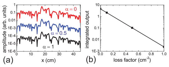
Figure 5: (a) Mode amplitude profile versus transverse distance for different values of the loss coefficient $\alpha$ after 350 mm of propagation. Red: $\alpha=0$ cm^-2. Blue: $\alpha=0.5$ cm^-2. Black: $\alpha=1$ cm^-2. (b) Integrated output versus loss coefficient on a semilog scale.

Our “open” experimental configuration requires that we first analyze the role of dissipation on transverse localization. The amplitude profile is calculated after 350 mm of propagation for a single realization of disorder for various values of $\alpha$ as shown in Fig. 5(a). For higher values of the absorption coefficient, the amplitude decreases, but the wave function shape does not alter. We conclude from these curves that absorption merely scales the wave intensity thereby supporting our experimental approach of studying transverse localization in the possible presence of out of plane losses. In Fig. 5(b), the integrated output is plotted versus the absorption coefficient. The output intensity clearly attenuates exponentially, confirming that dissipation only introduces an exponential scaling Weaver1993 . In Fig. 3(a), the mean of the participation length for an ensemble of 100 realizations of disorder is shown. This theoretical value for the waves extent falls within the standard deviation of the experimentally determined values.

Motivated by the experimentally observed and unforeseen excitation dependence of the wave functions, we also calculated the excitation-detection patterns. In Fig. 4(b), it is shown that the position and shape of these patterns correspond with the measurements. The anti-diagonal shapes are also clearly present in our numerical calculation, indicating that it is not caused by spurious effects such as mode perturbation due to the proximity of the receiver antenna.

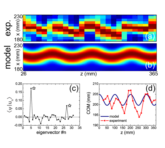
Figure 6: (a) Experimental and (b) calculated oscillations in the intensity profile for one sample excited at 10.2 GHz. Every column is normalized independently. (c) Expansion coefficients for the different eigenstates. Only two eigenstates, indicated by the stars, contribute significantly. (d) Center of mass of the intensity versus propagation direction for both the calculated and experimental data shown in (a) and (b).

An alternative analysis of the system in terms of eigenstates rather than the previous “brute force” numerical calculation has the advantage of reducing the problem’s complexity. When $\alpha=0$, the solutions to Eq. (2) can be written as a linear combination of the Hamiltonian’s eigenstates $u_{n}(x)$: $\psi(x,z)=\sum_{n}c_{n}u_{n}(x){\rm exp}(-i\lambda_{n}z)$, where $\lambda_{n}$ is the eigenvalue belonging to eigenstate $u_{n}$ and $c_{n}$ is the $n$’th expansion coefficient given by $c_{n}=\langle\psi|u_{n}\rangle$. The eigenstates and eigenvalues are calculated by diagonalizing a 598 $\times$ 598 matrix. The diagonal of the matrix contains the potential $k^{2}[n^{2}(x)-n_{0}^{2}]$ and the derivative in $x$ is approximated by using central differences creating a tridiagonal matrix when assuming absorbing boundary conditions.

In principle, diagonalizing a $N\times N$ matrix results in $N$ eigenvalues and eigenvectors. However, most of these eigenvectors contain too high spatial frequencies, $k_{n}>k$, that are not excitable in our system. As a result we end up with only 30 eigenstates that obey the relation $k_{n}\leq k$. This small number of modes in the system can lead to observable beatings of the system’s eigenstates in our two-dimensional spatial scans. Figure 6(a) shows a clear example of such oscillatory behavior of the wave function in experiment. A decomposition into the system eigenstates for this particular sample reveals just two eigenstates contribute significantly to the wave function as shown in Fig. 6(c). Using only these two eigenstates and their corresponding eigenvalues, we calculated the $z$-development of the wave function in Fig. 6(b) and compared them directly with experiment in Fig. 6(d). The calculated oscillations are quantitatively similar to those observed in experiment. In general, the number of significantly contributing eigenvectors is often higher than two, which makes the beating less visible. Yet, the anti-diagonal patterns shown in Fig. 4(a) and (b) are another observable consequence of the beating between the system’s eigenstates. Depending on the accumulated phase during propagation, these anti-diagonal excitation-detection patterns can in fact become circular or diagonal as shown in Fig. 4(c-e). The patterns are to a large extent point-symmetric which originates from a flip in sign of the expansion coefficients when the excitation antenna crosses the central position of the beating oscillation.

Conclusion and Discussion - We have measured how electromagnetic wave functions develop over time in localizing samples by carrying out a (1+1)D transverse localization experiment. Because of the limited number of modes in our system, the excitation can be described as a superposition of a few of the system’s eigenstates. The different eigenvalues of these eigenstates lead to observable beatings in wave functions.

We used out-of-plane scattering as an experimental analog of energy dissipation. The extent of the wave profiles is in quantitative agreement with calculations from a numerical solution to a Schrödinger type of equation. By introducing dissipation into this model, we deduce that dissipation is of no influence to the occurrence of transverse localization except for an exponential attenuation.

Since the transverse localization scheme allows for measuring snapshots of wave functions in time, it is a very convenient tool for studying the effect of different forms of disorder on wave propagation as put forward by recent work on photonic quasicrystals Silverberg2009 ; Segev2011 . Our work on transverse localization and dissipation suggests that transverse localization can also be an excellent platform for studying the influence of perturbations and partial incoherence on localization Buljan2011 .

- (1) P. W. Anderson, Phys. Rev. 109, 1492 (1958)
- (2) P. W. Anderson, Philos. Mag. B 52, 505 (1985)
- (3) S. John, Phys. Rev. Lett. 58, 2486 (1987)
- (4) A. A. Chabanov, M. Stoytchev, and A. Z. Genack, Nature 404, 850 (2000)
- (5) J. Wang and A. Z. Genack, Nature 471, 345 (2011)
- (6) H. Hu, A. Strybulevych, J. H. Page, S. E. Skipetrov, and B. A. van Tiggelen, Nat. Phys. 4, 945 (2008)
- (7) J. Billy, V. Josse, Z. Zuo, A. Bernard, B. Hambrecht, P. Lugan, D. Clément, L. Sanchez-Palencia, P. Bouyer, and A. Aspect, Nature 453, 891 (2009)
- (8) G. Roati, C. D’Errico, L. Fallani, M. Fattori, C. Fort, M. Z. G. Modugno, M. Modugno, and M. Inguscio, Nature 453, 895 (2009)
- (9) S. S. Kondov, W. R. McGehee, J. J. Zirbel, and B. DeMarco, Science 334, 66 (2011)
- (10) E. Abrahams, P. W. Anderson, D. C. Licciardello, and T. V. Ramakrishnan, Phys. Rev. Lett. 42, 673 (1979)
- (11) H. De Raedt, A. Lagendijk, and P. de Vries, Phys. Rev. Lett. 62, 47 (1989)
- (12) T. Schwartz, G. Bartal, S. Fishman, and M. Segev, Nature 446, 52 (2007)
- (13) Y. Lahini, A. Avidan, F. Pozzi, M. Sorel, R. Morandotti, D. N. Christodoulides, and Y. Silberberg, Phys. Rev. Lett. 100, 013906 (2008)
- (14) L. Levi, M. Rechtsman, B. Freedman, T. Schwartz, O. Manela, and M. Segev, Science 332, 1541 (2011)
- (15) S. Fishman, D. R. Grempel, and R. E. Prange, Phys. Rev. Lett. 49, 509 (1982)
- (16) F. L. Moore, J. C. Robinson, C. F. Bharucha, B. Sundaram, and M. G. Raizen, Phys. Rev. Lett. 75, 4598 (1995)
- (17) S. John, Phys. Rev. B 31, 304 (1985)
- (18) R. L. Weaver, Phys. Rev. B 47, 1077 (1993)
- (19) J. C. J. Paasschens, T. S. Misirpashaev, and C. W. J. Beenakker, Phys. Rev. B 54, 11887 (1996)
- (20) D. S. Wiersma, P. Bartolini, A. Lagendijk, and R. Righini, Nature 390, 671 (1997)
- (21) F. Scheffold, R. Lenke, R. Tweer, and G. Maret, Nature 398, 206 (1999)
- (22) Z. Q. Zhang, A. A. Chabanov, S. K. Cheung, C. H. Wong, and A. Z. Genack, Phys. Rev. B 79, 144203 (2009)
- (23) Hewlett-Packard, Measuring Dielectric Constant with the HP 8510 Network Analyzer (Hewlett-Packard, Pablo Alto, CA, 1985)
- (24) M. Rechtsman, A. Szameit, F. Dreisow, M. Heinrich, R. Keil, S. Nolte, and M. Segev, Phys. Rev. Lett. 106, 193904 (May 2011)
- (25) Y. V. Fyodorov and A. D. Mirlin, Phys. Rev. Lett. 71, 412 (1993)
- (26) W. E. Schiesser and G. W. Griffiths, A Compendium of Partial Differential Equation Models. Method of Lines Analysis with MatLab. (Cambridge University Press, 2009)
- (27) Y. Lahini, R. Pugatch, F. Pozzi, M. Sorel, R. Morandotti, N. Davidson, and Y. Silberberg, Phys. Rev. Lett. 103, 013901 (2009)
- (28) D. Čapeta, J. Radić, A. Szameit, M. Segev, and H. Buljan, Phys. Rev. A 84, 011801 (2011)