Motor-Driven Bacterial Flagella and Buckling Instabilities

Abstract

Many types of bacteria swim by rotating a bundle of helical filaments also called flagella. Each filament is driven by a rotary motor and a very flexible hook transmits the motor torque to the filament. We model it by discretizing Kirchhoff’s elastic-rod theory and develop a coarse-grained approach for driving the helical filament by a motor torque. A rotating flagellum generates a thrust force, which pushes the cell body forward and which increases with the motor torque. We fix the rotating flagellum in space and show that it buckles under the thrust force at a critical motor torque. Buckling becomes visible as a supercritical Hopf bifurcation in the thrust force. A second buckling transition occurs at an even higher motor torque. We attach the flagellum to a spherical cell body and also observe the first buckling transition during locomotion. By changing the size of the cell body, we vary the necessary thrust force and thereby obtain a characteristic relation between the critical thrust force and motor torque. We present a sophisticated analytical model for the buckling transition based on a helical rod which quantitatively reproduces the critical force-torque relation. Real values for motor torque, cell body size, and the geometry of the helical filament suggest that buckling should occur in single bacterial flagella. We also find that the orientation of pulling flagella along the driving torque is not stable and comment on the biological relevance for marine bacteria.

1 Introduction

Many bacteria such as Escherichia coli and Salmonella typhimurium swim by rotating a bundle of helical flagella Berg2004 . Nature’s simple and ingenious solution for locomotion at low Reynolds number has already inspired researchers to apply rotating flagella to perform such diverse tasks as pumping fluid Darnton2004 or manufacturing nanotubes Hesse2009 . Even artificial helical flagella already exist Zhang2009 .

The flagellum in the bundle consists of three parts; the rotary motor, a short and very flexible proximal hook that couples the motor to the third part, the long helical filament Berg2004 ; Turner2000 ; Darnton2007a . The motors are embedded at different locations of the cell wall so that the flagella have to bend around the cell body to form a bundle. Bacteria such as Escherichia coli and Salmonella typhimurium use this bundle to perform a run-and-tumble motion which enables them to follow a chemical gradient (chemotaxis). After swimming for about $1\mathrm{s}$, the sense of rotation of one motor reverses and the attached flagellum leaves the bundle. It goes through a sequence of polymorphic conformations until the motor reverses its rotational direction again. The flagellum returns to its original or normal helical form and rejoins the bundle. During this tumbling event, which lasts for about $0.1\mathrm{s}$, the bacterium changes its swimming direction randomly. It is interesting that flagella of cells, which are clued to a surface, do not bundle Darnton2007a ; Turner2000 . Furthermore, each flagellum is reported to be relatively rigid and visible deformations due to rotation are not reported Darnton2007a . In general, videos show a complex behavior of a single flagellum when it interacts with other flagella, with the wall, or when it goes through different polymorphic conformations Turner2000 . In this context, recent articles study the synchronization and bundling of two or more flagella due to hydrodynamic interactions Kim2003 ; Kim2004 ; Reichert2005 ; Janssen2011 .

The polymorphism of the flagellum is a fascinating and intensively studied subject asakura1970 ; calladine1975 ; Macnab1977 ; Hotani1982 ; Hasegawa1982 ; Goldstein2000 ; Srigiriraju2005 ; Darnton2007 ; Wada2008 . Using a coarse-grained molecular model, we recently addressed the question why the normal polymorphic state is realized in a flagellum Speier2011 and also developed a simple model for flagellar growth Schmitt2011 . Based on an extended Kirchhoff theory for the helical filament, we modeled the polymorphism of the flagellum Vogel2010 and were able to reproduce experimental force-extension curves where a polymorphic transition is induced by an external force Darnton2007 .

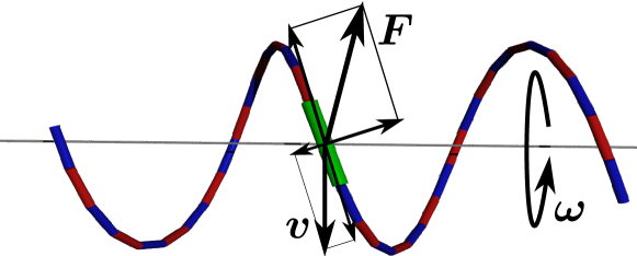
Figure 1: Each segment of a rotating helical flagellum experiences a frictional force $\boldsymbol{F}$ that is not antiparallel to the local velocity $\boldsymbol{v}$ due to the anisotropic friction of a rod. Whereas the force component perpendicular to the helix axis averages to zero over one helical turn, the parallel component adds up to the thrust force. For a detailed treatment see appendix A.

In this article we concentrate on the normal form of a single bacterial flagellum, model it by the discretized version of Kirchhoff’s elastic-rod theory and develop a coarse-grained approach for driving the helical filament by a motor torque. A rotating helical flagellum produces a thrust force as explained in fig. 1 that adds up along the filament and then pushes the cell body forward. We report two buckling instabilities of a fixed helical filament for increasing motor torque. The first instability occurs in the biologically relevant regime. The straight helical filament starts to bend under the influence of the acting thrust force similar to a rod that buckles under its own load. The buckling instability is visible as a supercritical Hopf bifurcation in the thrust force. It also occurs when the filament is allowed to move by attaching it to a load particle. We will develop an analytical model based on a rigid helical rod that explains the buckling transition and reproduces quantitatively the critical force-torque relation from our simulations.

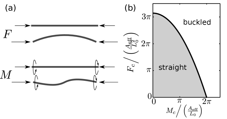
Figure 2: a) An elastic rod buckles under the influence of a compressional force $F$ and an external torque $M$. b) The critical values $F_{c}$ and $M_{c}$ at which buckling occurs obey a characteristic relation. The graph depicts relation (1) valid for a rod with fixed ends.

An elastic rod buckles under the influence of a compressional force and an external torque acting at both ends of the rod [fig. 2(a)]. This is one of the first examples for a bifurcation and Euler was the first to provide the theory for the critical load force at zero torque. In general, critical force and torque for a rod with fixed ends obey the relation Love1944

$$\pi^{2} =F_{c}\left(\frac{L_{0}^{2}}{A}\right)+\frac{1}{4}M_{c}^{2}\left(\frac{L_{0}}{A}\right)^{2},$$ (1)

where $L_{0}$ is the rod length and $A$ its bending rigidity [fig. 2(b)]. Note that eq. (1) does not depend on the compressibility or the torsional rigidity of the rod.

Similar buckling or elastic instabilities occur in the dynamics of rods at low Reynolds number. Here one typically applies a torque at one end of the filament. The rod rotates and the applied torque is balanced by frictional forces and torques continuously distributed along the filament. Wolgemuth et.al. investigated a rod with one clamped and one free end rotating around its axis. They observed two regimes separated by a supercritical (i.e. continues) Hopf bifurcation. When the rotational frequency exceeds a critical value, the straight filament starts to bend and performs a whirling motion Wolgemuth2000 . In Brownian dynamics simulations Wada and Netz observed for the same conditions a subcritical (i.e. discontinuous) Hopf bifurcation where the strongly bent filament nearly folds back on itself Wada2006 . On the other hand, a rod tilted with respect to the rotational axis bends slightly due to friction at low rotational velocity. At a critical value, a discontinuous transition to a helical rod shape occurs Manghi2006 .

In this article we treat buckling instabilities for the biologically relevant helical filament. The problem is more complex due to the characteristic rotation-translation coupling and the fact that we do not fix the orientation of the helical filament. The content of the article is organized as follows. In sect. 2 we explain how we model the motor-driven bacterial flagellum and how we perform the simulations. In sect. 3 we present and discuss our numerical results for both buckling instabilities for the fixed filament and then address the first buckling instability during locomotion of the filament. In sect. 4 we formulate a buckling theory for a helical rod and show that it quantitatively reproduces the critical force-torque relation in the biologically relevant regime. We close with a summary and conclusions.

2 Modeling the motor-driven bacterial flagellum

We start with a short review of the elasticity model and the dynamics of a helical filament in sects. 2.1 and 2.2 following our previous work Vogel2010 and then explain how we model the motor-driven hook in sect. 2.3. A summary of the simulation parameters follows in sect. 2.4.

2.1 Elasticity model of a helical filament

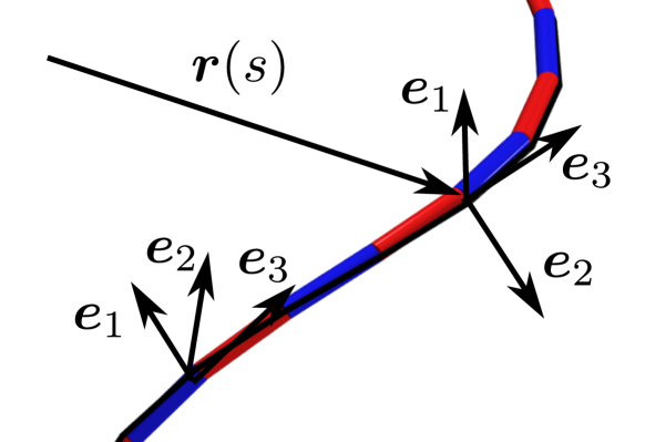
Figure 3: The kinematic variables of a slender elastic rod are the space curve $\boldsymbol{r}(s)$ of its center line and the material frame $\{\boldsymbol{e}_{1},\boldsymbol{e}_{2},\boldsymbol{e}_{3}\}$ attached at each point of the center line.

We describe the conformation of the helical filament with contour length $L$ by the space curve of its center line $\boldsymbol{r}(s)$, where $s$ is the arc length. In addition, we attach a material frame of three orthogonal unit vectors $\{\boldsymbol{e}_{1},\boldsymbol{e}_{2},\boldsymbol{e}_{3}\}$, to each point along the filament so that $\boldsymbol{e}_{3}$ points along the tangent of $\boldsymbol{r}(s)$ (see fig. 3). The generalized Frenet-Serret equations transport the material frame along the filament,

$$\partial_{s}\boldsymbol{e}_{i}=\boldsymbol{\Omega}\times\boldsymbol{e}_{i},$$ (2)

where $\partial_{s}$ means derivative with respect to $s$. We can characterize any conformation by the angular strain vector $\boldsymbol{\Omega}=(\Omega_{1},\Omega_{2},\Omega_{3})$ given in components with respect to the local material frame. Along an ideal helical filament, spontaneous curvature $\kappa_{0}$ and torsion $\tau_{0}$ are constant. As material frame for the equilibrium shape of the helical filament, we choose the Frenet frame which consists of the tangent vector $\boldsymbol{t}=\boldsymbol{e}_{3}$, the normal vector $\boldsymbol{e}_{1}=\boldsymbol{n}=\partial_{s}\boldsymbol{t}/\kappa_{0}$, and the binormal vector $\boldsymbol{e}_{2}=\boldsymbol{b}=\boldsymbol{t}\times\boldsymbol{n}$. The strain vector then becomes $\boldsymbol{\Omega}=(0,\kappa_{0},\tau_{0})$. Further parameters of an ideal helix are the pitch $p=2\pi\tau_{0}/(\kappa_{0}^{2}+\tau_{0}^{2})$ and radius $R=\kappa_{0}/(\kappa_{0}^{2}+\tau_{0}^{2})$. The ratio of pitch and circumference, $p/2\pi R=\tan\alpha$, defines the pitch angle $\alpha$.

The total elastic free energy of the filament consists of two contributions:

$${\mathcal{F}}=\int_{0}^{L}(f_{\mathtt{cl}}+f_{\mathtt{st}})\mathrm{d}s$$ (3)

The first term is Kirchhoff’s classical theory for bending and twisting,

$$f_{\mathtt{cl}}=\frac{A}{2}(\Omega_{1})^{2}+\frac{A}{2}(\Omega_{2}-\kappa_{0})^{2}+\frac{C}{2}(\Omega_{3}-\tau_{0})^{2},$$ (4)

where we introduced the bending rigidity $A$ and the torsional rigidity $C$ Love1944 ; Landau1986 . Instead of implementing a constraint for the inextensibility of the filament in our simulations, we also add a stretching free energy with line density

$$f_{\mathtt{st}}=\frac{K}{2}\left(\partial_{s}\boldsymbol{r}\right)^{2}.$$ (5)

We choose the spring constant $K$ such that the changes in the filament length are below 1.5 %. The filament is inextensible to a good approximation.

2.2 Dynamics of the helical filament

We mostly performed deterministic simulations, only in a few cases we have added thermal fluctuations. We formulate Langevin equations for the location $\boldsymbol{r}(s)$ and intrinsic twist $\phi(s)$ of the helical filament. At low Reynolds number elastic force per unit length, $\boldsymbol{f}_{\mathtt{el}}=-\delta\cal F/\delta\boldsymbol{r}$, and thermal force $\boldsymbol{f}_{\mathtt{th}}$ are balanced by viscous drag. The same applies to the elastic torque per unit length, $m_{\mathtt{el}}=-\delta\cal F/\delta\phi$ and thermal torque $m_{\mathtt{th}}$. Using resistive-force theory, we introduce local friction coefficients $\gamma_{\parallel},\gamma_{\perp}$ and $\gamma_{R}$ (see Appendix A) and arrive at the Langevin equations

$$\left[\gamma_{\parallel}\boldsymbol{t}\otimes\boldsymbol{t}+\gamma_{\perp}(\boldsymbol{\sf 1}-\boldsymbol{t}\otimes\boldsymbol{t})\right]\boldsymbol{v}= \boldsymbol{f}_{\mathtt{el}}+\boldsymbol{f}_{\mathtt{th}}$$ (6)

$$\gamma_{R}\omega= m_{\mathtt{el}}+m_{\mathtt{th}}.$$ (7)

Here $\boldsymbol{v}=\partial_{t}\boldsymbol{r}$ is the translational velocity, $\omega=\partial_{t}\phi$ the angular velocity about the local tangent vector $\boldsymbol{t}=\boldsymbol{e}_{3}$, and $\otimes$ means tensorial product. The anisotropic friction tensor acting on $\boldsymbol{v}$ in Eq. (6) couples rotation about the helical axis to translation and thereby creates the thrust force that pushes the bacterium forward as illustrated in fig. 1 Purcell1977 . Experiments show reasonable agreement with the approach of resistive-force theory Chattopadhyay2006 ; Chattopadhyay2009 . Finally, the thermal force $\boldsymbol{f}_{\mathtt{th}}$ and torque $m_{\mathtt{th}}$ are Gaussian stochastic variables with zero mean, $\langle\boldsymbol{f}_{\mathtt{th}}\rangle=\boldsymbol{0}$ and $\langle m_{\mathtt{th}}\rangle=0$. Their variances obey the fluctuation-dissipation theorem and therefore read

$$\left\langle\boldsymbol{f}_{\mathtt{th}}(t,s)\otimes\boldsymbol{f}_{\mathtt{th}}(t^{\prime},s^{\prime})\right\rangle =2k_{B}T\delta(t-t^{\prime})\delta(s-s^{\prime})$$ (8)

$$\times\left[\gamma_{\parallel}\boldsymbol{t}\otimes\boldsymbol{t}+\gamma_{\perp}(\boldsymbol{\sf 1}-\boldsymbol{t}\otimes\boldsymbol{t})\right],$$

$$\left\langle m_{\mathtt{th}}(t,s)m_{\mathtt{th}}(t^{\prime},s^{\prime})\right\rangle =2k_{B}T\delta(t-t^{\prime})\delta(s-s^{\prime})\gamma_{R},$$ (9)

$$\left\langle m_{\mathtt{th}}(t,s)\boldsymbol{f}_{\mathtt{th}}(t^{\prime},s^{\prime})\right\rangle =\boldsymbol{0}.$$ (10)

In our simulations we use a discretized version of the dynamic equations following our earlier work Reichert2006 ; Vogel2010 (see also Ref. Chirico1994 ; Wada2007a ; Wada2007 ). We discretize the center line $\boldsymbol{r}(s)$ of the filament by introducing $N+1$ beads at locations $\boldsymbol{r}^{(i)}=\boldsymbol{r}(s=i\cdot h)$ and with nearest-neighbor distance $h$. To every bead we attach the material frame $\{\boldsymbol{e}^{(i)}_{1},\boldsymbol{e}^{(i)}_{2},\boldsymbol{e}^{(i)}_{3}\}$ ($i=0,\dots,N$) and approximate the tangent vector by

$$\boldsymbol{e}_{3}^{(i)} =\frac{\boldsymbol{r}^{(i)}-\boldsymbol{r}^{(i-1)}}{|\boldsymbol{r}^{(i)}-\boldsymbol{r}^{(i-1)}|}.$$ (11)

The transport of the material frame along the filament occurs in two steps: First, we rotate about the bond direction $\boldsymbol{e}^{(i)}_{3}$ by an angle $\Omega_{3}^{(i)}h$ to implement intrinsic twist plus torsion. Thereafter, we introduce the curvature of the filament, by rotating the the bond vector $\boldsymbol{e}_{3}^{(i)}$ of the material frame about $\boldsymbol{e}_{3}^{(i)}\times\boldsymbol{e}_{3}^{(i+1)}$ by an angle $\sqrt{\Omega_{1}^{2}+\Omega_{2}^{2}}h$ into the consecutive direction $\boldsymbol{e}_{3}^{(i+1)}$. With this procedure the free energy densities $f_{\mathtt{cl}}$ and $f_{\mathtt{st}}$ from Eqs. (4) and (5) are discretized and the functional derivatives of the total free energy, $\boldsymbol{f}_{\mathtt{el}}=-\delta\cal F/\delta\boldsymbol{r}$ and $m_{\mathtt{el}}=-\delta\cal F/\delta\phi$, reduce to conventional derivatives with respect to $\boldsymbol{r}^{(i)}$ and $\phi^{(i)}$. In addition, we approximate the tangent vector in the friction tensor in Eq. (6) by $\boldsymbol{t}^{(i)}=(\boldsymbol{e}_{3}^{(i)}+\boldsymbol{e}_{3}^{(i+1)})/|\boldsymbol{e}_{3}^{(i)}+\boldsymbol{e}_{3}^{(i+1)}|$.

2.3 The motor-driven hook

The flagellum is driven by a rotary motor embedded in the cell wall of the bacterium. The motor torque is transmitted to the helical filament by a short flexible coupling. Because of its shape it is called hook. With a well regulated length of $0.05\mathrm{\SIUnitSymbolMicro}\mathrm{m}$ for E.Coli or S.typhimurium and up to $0.1\mathrm{\SIUnitSymbolMicro}\mathrm{m}$ for R. sphaeroides it is much shorter than the helical filament Jones1990 ; Kobayashi2003 ; Samatey2004 ; Shaikh2005 . It is also shorter than the discretization length of $h=0.2\mathrm{\SIUnitSymbolMicro}\mathrm{m}$ which we can employ in our simulations as indicated in fig. 4. We, therefore, cannot model the hook in full detail. Instead, we represent motor and hook by a motor torque that acts directly on one end of the filament neglecting the extension of the hook.

Molecular dynamics simulations showed that the hook bends and twists easily. This is possible since conformational changes of molecular bonds require only a small amount of energy Furuta2007 . So the hook itself allows the filament to nearly assume any orientation outside the cell. Hence, it is comparable to a constant-velocity joint. The blow-up in fig. 4 illustrates how motor and hook act together to drive the filament. The picture also shows the rotational degrees of freedom of the filament at the attachment point to the hook. The filament can rotate about its local axis, about the axis parallel to the motor torque, and towards or away from this axis.

The task of the hook is to transmit the motor torque to the filament and to guarantee its rotational degrees of freedom. In our coarse-grained model, we implement this task by balancing all the torques acting on the first material frame $\{\boldsymbol{e}_{1}^{(0)},\boldsymbol{e}_{2}^{(0)},\boldsymbol{e}_{3}^{(0)}\}$ that determines the orientation of one end of the filament:

$$\big{[}\gamma_{R}h \boldsymbol{e}_{3}^{(0)}\boldsymbol{e}_{3}^{(0)}+\frac{1}{2}\gamma_{\perp}h^{3}(\boldsymbol{\sf 1}-\boldsymbol{e}_{3}^{(0)}\boldsymbol{e}_{3}^{(0)})\big{]}\boldsymbol{\omega}$$ (12)

$$= \boldsymbol{M}-A[\Omega_{1}\boldsymbol{e}_{1}^{(0)}+(\Omega_{2}-\kappa_{0})\boldsymbol{e}_{2}^{(0)}]-C(\Omega_{3}-\tau_{0})\boldsymbol{e}_{3}^{(0)}.$$

The material frame rotates with an angular frequency $\boldsymbol{\omega}$. It gives rise to a frictional torque decomposed into a component along the tangent vector $\boldsymbol{e}_{3}^{(0)}$ and perpendicular to it. The length $h$ appears due to the discretization. The frictional torque is balanced by the motor or external torque $\boldsymbol{M}=M\boldsymbol{e}_{z}$, which we assume constant throughout the paper, and the elastic torque $-\delta{\mathcal{F}}/\delta\boldsymbol{\Omega}$.

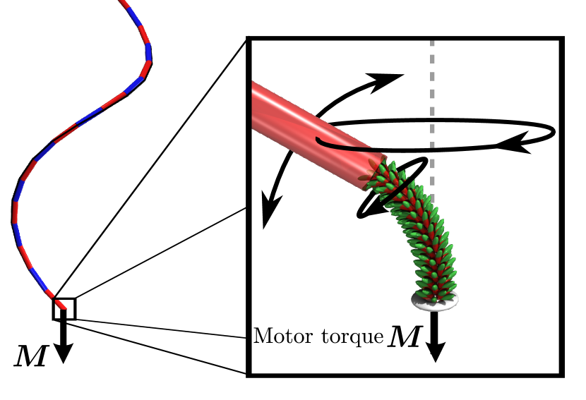
Figure 4: Blow-up: The hook acts as a universal joint between the motor embedded in the cell wall and the long helical filament which retains its full rotational degrees of freedom. Main picture: The hook is much shorter than the discretization length indicated by the blue and red segments of the filament. We do not model the hook explicitly but let the motor torque act directly on the first material frame of the filament which, in principle, can assume any orientation in space.

2.4 Simulation parameters

For the bending rigidity we use $A=3.5\mathrm{p}\mathrm{N}\mathrm{\SIUnitSymbolMicro}\mathrm{m}^{2}$ given in Ref. Darnton2007 as a typical value for bacterial flagella and set it equal to the torsional rigidity, $C=A$. Our previous work showed that this is in agreement with experimental observations Vogel2010 . All other parameters are determined by the geometry. In our study we use the normal state of the bacterial flagellum with spontaneous curvature $\kappa_{1}=1.3\mathrm{/}\mathrm{\SIUnitSymbolMicro}\mathrm{m}$ and torsion $\tau_{1}=2.1\mathrm{/}\mathrm{\SIUnitSymbolMicro}\mathrm{m}$. In the following we study a right-handed helical filament although the normal state of a real flagellum is left-handed. We calculate the local friction coefficients from Lighthill’s formulas Lighthill1976 summarized in appendix A as $\gamma_{\parallel}=1.6\cdot 10^{-3}\mathrm{p}\mathrm{N}\mathrm{s}\mathrm{/}\mathrm{\SIUnitSymbolMicro}\mathrm{m}^{2}$, $\gamma_{\perp}=2.8\cdot 10^{-3}\mathrm{p}\mathrm{N}\mathrm{s}\mathrm{/}\mathrm{\SIUnitSymbolMicro}\mathrm{m}^{2}$, and $\gamma_{R}=1.26\cdot 10^{-6}\mathrm{p}\mathrm{N}\mathrm{s}$, where a filament diameter of about $20\mathrm{n}\mathrm{m}$ is used. The length of the filament is $L=10\mathrm{\SIUnitSymbolMicro}\mathrm{m}$ corresponding to approximately four helical turns. The discretization length between the beads is chosen as $h=0.2\mathrm{\SIUnitSymbolMicro}\mathrm{m}$.

3 The motor-driven helical filament

In this section we study in detail the thrust force that the motor-driven helical filament generates both when the actuated end of the filament is fixed in space or attached to a larger load particle, which mimics the cell body. In particular, we describe the buckling transitions by illustrating the observed filament configurations.

It is instructive to shortly look at a completely rigid helical rod first, which does not exhibit translational motion. In the low Reynolds number regime, the angular velocity $\boldsymbol{\omega}$ of the rod and the applied torque $\boldsymbol{M}$ obey the linear relation $\boldsymbol{M}=\boldsymbol{\sf B}\boldsymbol{\omega},$ where $\boldsymbol{\sf B}$ is the rotational friction tensor. For a long slender helix like the normal form of the bacterial filament, one principal axis of $\boldsymbol{\sf B}$ points along the helical axis and the eigenvalues in the plane perpendicular to this axis are degenerate, in good approximation Lighthill1976 ; Childress1981 . Now there is a formal analogy to the motion of the force and torque less spinning top with axial symmetry in classical mechanics Landau1976 ; Arnold1978 . We just replace the constant torque $\boldsymbol{M}$ by the conserved angular momentum and $\boldsymbol{\sf B}$ by the moment of inertia tensor. We explain details in appendix B. According to this analogy, the rigid helix in a viscous fluids precesses about the constant applied torque while also rotating about its helical axis. However, in our simulations we observe that as soon as we introduce a finite elasticity of the helical rod, the precession is no longer stable and the helical filament aligns, for example, parallel to the torque.

3.1 Force-torque relation and buckling

3.1.1 Discussion of the basic features

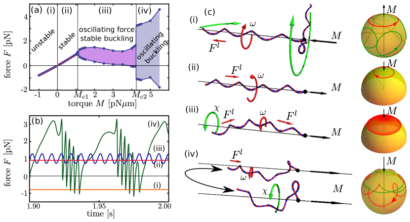
Figure 5: (a) Thrust force $F$ versus motor torque $M$. Four different regimes associated with different configurations of the rotating filament exist. In regime (iii) and (iv) the minimum and maximum value of the oscillating thrust force are shown. A supercritical bifurcation occurs at the critical torque $M_{c1}\approx 1.1\mathrm{p}\mathrm{N}\mathrm{\SIUnitSymbolMicro}\mathrm{m}$ indicating a buckling transition. A second bifurcation is visible at $M_{c2}\approx 4.2\mathrm{p}\mathrm{N}\mathrm{\SIUnitSymbolMicro}\mathrm{m}$. The red line in regimes (i) and (ii) follows from resistive force theory. (b) Thrust force versus time for specific torque values in the four different regimes: (i) $M=-1.0\mathrm{p}\mathrm{N}\mathrm{\SIUnitSymbolMicro}\mathrm{m}$, (ii) $M=1.0\mathrm{p}\mathrm{N}\mathrm{\SIUnitSymbolMicro}\mathrm{m}$, (iii) $M=1.2\mathrm{p}\mathrm{N}\mathrm{\SIUnitSymbolMicro}\mathrm{m}$, and (iv) $M=4.5\mathrm{p}\mathrm{N}\mathrm{\SIUnitSymbolMicro}\mathrm{m}$. (c) Characteristic snapshots of the helical filament in the four regimes. The red circular arrow and $\omega$ indicate a rotation about the local helix axis and $F^{l}$ the local thrust force. The green circular arrow and $\chi$ show the precession about the external torque axis. In addition, the trajectory of the tip of the first tangent vector is indicated: (i) The green line belongs to the perpendicular orientation of the filament, (iv) red line: fast rotation about helical axis, green line: slow precession about motor torque during relaxation of the filament.

The motor-driven helical filament creates a thrust force. We calculate it as the force component on the first bead parallel to the applied torque $\boldsymbol{M}=M\boldsymbol{e}_{z}$: $F=-\partial\mathcal{F}/\partial\boldsymbol{r}^{(0)}\cdot\boldsymbol{e}_{z}$. We keep here the bead at a fixed position $\boldsymbol{r}^{0}=\boldsymbol{r}(0)$ and use the discretized version of the free energy (4). Figure 5(a) plots the resulting thrust force $F$ versus the applied torque determined in simulations without thermal noise. We discuss the graph in detail.

A positive torque $M$ produces a thrust force that pushes against the anchoring point of the filament. The thrust force is constant in time as indicated by the straight line (ii) in fig. 5(b). The illustration (ii) of fig. 5(c) shows the stable orientation of the helical filament along the torque $\boldsymbol{M}$. It rotates about the helical axis with angular frequency $\boldsymbol{\omega}$. The local thrust force acting along the helix axis is indicated by $F^{l}$. The tangent of the filament at the anchoring point is tilted against $\boldsymbol{M}$ and the tip moves on a circle, as indicated by the schematic. Movies for all four types of configurations are available in the supplemental material.

A negative torque $M$ generates a negative force that pulls at the anchoring point. However, we realized that the orientation of the filament along the torque is not stable. For long times the filament turns away from the torque axis [green arrow in illustration (i) of fig. 5(c)] until it reaches a configuration perpendicular to $\boldsymbol{M}$, where it slowly rotates about the local helical axis and slowly precesses about $\boldsymbol{M}$. This motion is also visible for the tip of the first tangent vector. The linear increase of $F$ with $M$ in the regimes (i) and (ii) in fig. 5(a) fits well with the result from resistive force theory for a perfect helical filament, as indicated by the line (see appendix A). Small deviations are visible at higher torques due to elastic deformations of the helix which enhance the thrust force.

At a critical torque $M_{c1}\approx 1.1\mathrm{p}\mathrm{N}\mathrm{\SIUnitSymbolMicro}\mathrm{m}$ the thrust force starts to oscillate as curve (iii) in fig. 5(c) indicates. Minimum and maximum values of the force are plotted in fig. 5(a). They develop continuously from the constant force at $M_{c1}$ indicating a supercritical Hopf bifurcation. Illustration (iii) of fig. 5(c) shows a buckled configuration that rotates about the local helix axis with frequency $\omega$ and precesses with frequency $\chi$ about the motor torque $\boldsymbol{M}$ keeping its shape fixed. The trajectory of the tip of the first tangent vector reflects this motion. A straightforward explanation is that the helical filament buckles under the thrust force generated by the rotating filament. The force adds up from the free to the fixed end of the filament and puts the filament under compressional tension. This is similar to a rod that buckles under its own gravitational load Love1944 ; Landau1986 . In sect. 4 we will develop a theory for this buckling transition which is quite involved. Finally, at a critical torque value of $M_{c2}\approx 4.2\mathrm{p}\mathrm{N}\mathrm{\SIUnitSymbolMicro}\mathrm{m}$ a second bifurcation occurs in the force-torque relation of fig. 5(a). The buckled state itself becomes unstable, visible by the fast oscillations of the thrust force in fig. 5(b). The buckled configuration is compressed until the fixed end becomes perpendicular to the motor torque. At this point the fast rotation about the local helical axis stops and the thrust force averaged over one fast period is approximately zero. Now the strongly bent configuration of the filament relaxes slowly and precesses about the applied torque $\boldsymbol{M}$ [second configuration in fig. 5(b)(iv)]. The thrust force on the anchoring point slowly increases. When the filament is sufficiently relaxed, it starts again its fast rotations about the local helix axis and the whole cycle repeats.

3.1.2 Discussion of additional features

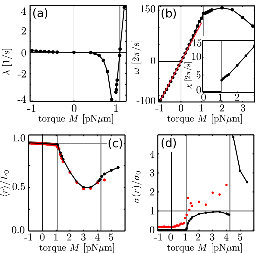
Figure 6: (a) Relaxation rate $\lambda$ of the elastic free energy versus applied torque $M$ for a small disturbance of the aligned state where the filament is parallel to the torque direction. (b) Angular velocity $\omega$ and precession frequency $\chi$ versus torque $M$. The supercritical bifurcation at $M_{c1}$ is clearly visible. The red line is calculated with resistive force theory. (c) Mean end-to-end distance $\langle r\rangle$ in units of the helix length $L_{0}$ versus $M$. The red dots are results from Brownian dynamics simulations with thermal noise included. (d) Standard deviation $\sigma(r)$ of the end-to-end distance in units of $\sigma_{0}=R/\sqrt{2}$ versus $M$. Thermal noise (red dots) leads to fluctuations about the mean value.

The reported supercritical Hopf bifurcation is also visible in other quantities besides the thrust force. We discuss here additional properties of the motor-driven helical filament.

To quantify the stability of the filament aligned parallel to the motor torque axis, we recorded the temporal evolution of the elastic free energy starting from a small disturbance of the aligned state and fit it to the form

$$\lvert\mathcal{F}-\mathcal{F}^{0}\rvert \approx\delta\mathcal{F}^{0}\exp(\lambda t)\sin(\omega t).$$ (13)

Here $\omega$ is the angular velocity of the rotating helix leading to oscillations in $\mathcal{F}$ and $\lambda$ is the reorientation rate. The result for $\lambda$ is plotted in fig. 6(a). For positive $M$ below the critical torque, the negative $\lambda$ indicates the stable aligned state. For small $M$ a reorientation of the filament could not be detected within the simulation time. Frictional forces are small and hardly deform the helix which, therefore, just precesses about the applied torque. Nevertheless, to record the thrust force-torque relation, we always started from an aligned state at $M=1\mathrm{p}\mathrm{N}\mathrm{\SIUnitSymbolMicro}\mathrm{m}$ and then changed the driving torque to the desired value and let the elastic free energy relax to its stationary value, where we finally recorded the thrust force. The small positive $\lambda$ for $M<0$ indicates the slow reorientation of the filament towards the perpendicular configuration The supercritical Hopf bifurcation is located where $\lambda$ changes sign from negative to positive.

Figure 6(b) shows the angular frequency $\omega$ for rotations about the local helix axis as a function of $M$. The linear regime belongs to the aligned state, deviations from it occur in the buckled state. The precession frequency $\chi$ for rotations of the whole filament about the torque axis is plotted in the inset. A non-zero $\chi$ corresponds to the buckled state.

Finally, figs. 6(c) and (d) plot the mean end-to-end distance $\langle r\rangle$ of the helix and its standard deviation $\sigma$ as a function of $M$, respectively. They are defined as

$$\langle r\rangle =\lim_{T\to\infty}\frac{1}{T}\int_{0}^{T}\lvert\boldsymbol{r}(s=L)-\boldsymbol{r}(s=0)\rvert\text{d}t$$ (14)

$$\sigma^{2} =\left\langle(r-\langle r\rangle)^{2}\right\rangle.$$ (15)

Whereas $\langle r\rangle$ is continuous at both bifurcations, the standard deviation displays a pronounced discontinuity at the second bifurcation in agreement with the behavior of the thrust force. We write $\sigma$ in units of $\sigma_{0}=R/\sqrt{2}$, where $R$ is the helix radius. $\sigma_{0}$ is the maximum value of $\sigma$ in regime (iii) where the buckled helix has a constant shape but the free end of the filament rotates on a circle with radius $R$. The strong increase of $\sigma$ in regime (iv) is due to the oscillating buckled state.

The rotating filament also experiences thermal forces due to the viscous environment. However, since the persistence length $A/k_{B}T\approx 1\mathrm{m}\mathrm{m}$ calculated from the bending rigidity $A$ is much larger than the filament length of $10\mu\mathrm{m}$, we do expect that our results are robust against thermal fluctuations. This is confirmed by the end-to-end distance $\langle r\rangle$ in fig. 6(c) (red dots) which agrees with the deterministic simulations. The standard deviation in 6(d) indicates some fluctuations. Below the buckling transition we can directly connect them to compressional fluctuations using the spring constant of the helical filament, $A/(R^{2}L)$, calculated in our earlier article Vogel2010 . The equipartition theorem gives $\sigma/\sigma_{0}\approx 0.15$ in good agreement with the simulated value of 0.18. In the buckled state, the helical filament has more opportunities to fluctuate around which explains the further increase of $\sigma$. Furthermore, we observe strong fluctuations of the thrust force in our simulations which result from the delta correlated stochastic forces acting on the fixed first bead of the discretized filament. An average over these fluctuations agrees with the deterministic case (data not shown). The fluctuations will also be smoothed out in an experiment which performs some temporal average during measurement.

3.2 Buckling instability during locomotion

So far we have studied the situation where one end of the filament is fixed in space so that it cannot translate. However, rotating flagella push the cell body of a bacterium forward so that it moves. We mimic this scenario by attaching the filament to a bead of radius $a$ which, for simplicity, can only move along the $z$ direction. The thrust force $F$ generated at the attached end of the filament is then used to push the sphere forward acting against the Stokes friction force. We observe similar thrust force-torque relations as for the case of a fixed filament. The aligned state is again unstable for negative torque and possesses a larger reorientation rate which might have biological relevance as we discuss in sect. 5. For positive torque, the aligned state is stable and the thrust force grows linearly in the driving torque $M$ until the Hopf bifurcation occurs at a critical value $M_{c1}$ indicating the buckling instability.

Figure 7(a) shows the critical torque $M_{c1}$ as a function of the inverse bead radius $1/a$. From $1/a=0$, which corresponds to the fixed filament, the critical torque increases linearly in $1/a$ and then at $a^{-1}\approx 5/2$ turns into a slow growth towards the value for the freely swimming helix, i.e., $1/a\rightarrow\infty$. In the biological relevant case with the cell body size $a\approx 0.5\cdots 2\mathrm{\SIUnitSymbolMicro}\mathrm{m}$, the linear dependence of the critical torque on $1/a$ can be derived based on the fact that the critical thrust force $F_{c1}$ is nearly constant, as we show in fig. 7(b). So the velocity $v=F_{c1}/(6\pi\eta a)$ is so slow that the buckling transition is hardly influenced by the motion of the helical filament with the attached bead. Now, force and torque on the helix depend linearly on velocity $v$ and angular velocity $\omega$ (see appendix A). Eliminating $\omega$ and setting $v=F_{c1}/(6\pi\eta a)$ at the buckling transition, one arrives at

$$M_{c1}=-\frac{B_{\parallel}}{C_{\parallel}}F_{c1}+\left(C_{\parallel}-\frac{A_{\parallel}B_{\parallel}}{C_{\parallel}}\right)\frac{F_{c1}}{6\pi\eta}\frac{1}{a}.$$ (16)

Here $A_{\parallel}$, $B_{\parallel}$, and $C_{\parallel}$ are the translational, the rotational, and coupling friction coefficients parallel to the helical axis, respectively. This formula with the coefficients calculated by resistive force theory (see appendix A) reproduces the linear increase for small $1/a$, as demonstrated by the red line in the inset of fig. 7(a).

In fig. 7(b) we plot the critical thrust force versus the critical torque. For biologically relevant values $M_{c1}$ between $1$ and $2\mathrm{p}\mathrm{N}\mathrm{\SIUnitSymbolMicro}\mathrm{m}$ the critical force is indeed nearly constant. It only shows a very slow linear increase since frictional forces due to the motion of the helix stabilize it against buckling. At $M_{c1}\approx 4\mathrm{p}\mathrm{N}\mathrm{\SIUnitSymbolMicro}\mathrm{m}$ the behavior changes dramatically. The critical thrust force goes to zero proportional to $M_{c1}^{2}$ (see dotted line) following the behavior of a rod that buckles under an applied force and torque as described in the introduction. In this regime the supercritical Hopf bifurcation becomes subcritical and hysteresis occurs. So whereas for small torques buckling is hindered by locomotion, for large torque the typical quadratic dependence $F_{c1}\propto M_{c1}^{2}$ is observed. In the following section, we develop a theory to describe the observed buckling transition.

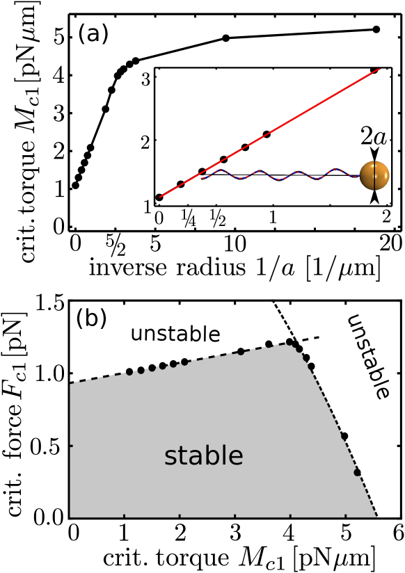
Figure 7: Buckling transition for a helical filament attached to a bead of radius $a$ that can move along the $z$ direction. (a) Critical torque $M_{c1}$ as a function of inverse bead radius $1/a$. Inset: Blow-up for the biologically relevant regime. (b) Critical force $F_{c1}$ versus critical torque $M_{c1}$.

4 Buckling theory for a helical rod

The goal in this section is to formulate a theory that reproduces the force-torque relation in fig. 7(b) for the first buckling transition of the helical filament as obtained by our simulations. Clearly, this relation cannot directly be explained by the theory of a thin elastic rod that buckles under the influence of an external force and torque which we shortly mentioned in the introduction in Eq. (1). There are several reasons for this. First, the helical filament is not just a simple elastic rod. Second, the external force that puts the helix under tension is generated locally by the rotation-translation coupling of the helix and accumulated along the filament similar to a rod that buckles under its own gravitational weight. Third, the whole filament moves with a constant velocity which leads to additional frictional forces and it also precesses about the external torque in the buckled state. In the following we formulate a model based on the theory of a thin elastic helical rod, derive from it a force-torque relation for the buckling transition, and compare it to fig. 7(b).

4.1 Model equations

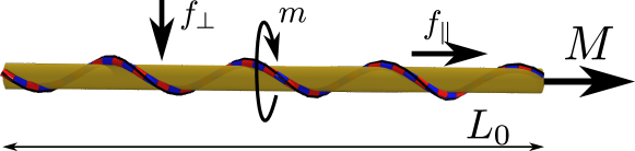
Figure 8: The helical filament is approximated by a thin helical rod of length $L_{0}$ that is characterized by the effective bending rigidity $A_{\text{eff}}$ and local friction coefficients of the helical filament. The applied torque $M\boldsymbol{e}_{z}$ generates the frictional torque $m$ and forces $f_{\parallel}$ and $f_{\perp}$.

To set up our model equations, we approximate the helical filament by a thin helical rod where the helicity comes in through the rotation-translation coupling in the friction matrix. The length of the rod, $L_{0}=\sin\alpha L$, agrees with the height of the helix, where $\alpha$ is the pitch angle. In engineering science the buckling of helical springs is a well known problem. If the height of the spring is larger than its radius, one approximates the spring by a soft rod with effective bending, shear, and compressional rigidity Haringx1942 ; Haringx1948 ; Biezeno1939 . In our case, in contrast to classical helical spring theory, the pitch of the helix is much larger than its radius. We therefore had to generalize the theory of helical springs in Ref. Biezeno1939 to derive an effective bending rigidity of the helical rod in terms of the bending and torsional rigidity of the filament:

$$\frac{1}{A_{\text{eff}}} =\frac{1}{2}\frac{1}{A}\frac{1}{\sin\alpha}\left(1+\sin^{2}\alpha+\frac{A}{C}\cos^{2}\alpha\right)$$ (17)

Details of the derivation are given in appendix C.

To address buckling of the helical rod, we start with the balance equations for force and momentum acting on a thin elastic rod Love1944 ; Landau1986 and neglect any inertial contribution in the low Reynolds number regime:

$$\boldsymbol{F}^{\prime}+\boldsymbol{f} =0,$$ (18a)

$$\boldsymbol{M}^{\prime}+\boldsymbol{e}_{3}\times\boldsymbol{F}+\boldsymbol{m} =0,$$ (18b)

where ^′ means derivative with respect to the arc length $s$ and $\boldsymbol{e}_{3}$ is the local tangent vector. Here $\boldsymbol{F}$ and $\boldsymbol{M}$ are internal elastic forces and torques acting along the rod, whereas $\boldsymbol{f}$ and $\boldsymbol{m}$ denote, respectively, external force and torque densities due to the applied motor torque and friction with the surrounding fluid. In addition, boundary conditions are necessary. At the free end of the rod ($s=L_{0}$) no external force and torque act, so elastic force and torque have to vanish. The end attached to the sphere can only move in $z$ direction with velocity $v$. The external torque $M\boldsymbol{e}_{z}$ is balanced by the elastic torque $\boldsymbol{M}(0)$ and the thrust force on the sphere $F=6\pi\eta av$ equals the elastic force at the leading end of the rod, $F_{z}(0)$:

$$F_{z}(0) =F=6\pi\eta av\boldsymbol{e}_{z}, \boldsymbol{M}(0) =M\boldsymbol{e}_{z},$$ (19a)

$$\boldsymbol{F}(L_{0}) =\boldsymbol{0}, \boldsymbol{M}(L_{0}) =\boldsymbol{0}.$$ (19b)

After setting up the problem, we have to explain how the different forces and torques entering Eqs. (18) look like for the helical rod close to the buckling transition. The elastic torque $\boldsymbol{M}$ is proportional to the angular strain vector $\boldsymbol{\Omega}$ written in components with respect to the local material frame $\{\boldsymbol{e}_{1},\boldsymbol{e}_{2},\boldsymbol{e}_{3}\}$:

$$\boldsymbol{M} =A_{\text{eff}}\Omega_{1}\boldsymbol{e}_{1}+A_{\text{eff}}\Omega_{2}\boldsymbol{e}_{2}+C_{\text{eff}}\Omega_{3}\boldsymbol{e}_{3},$$ (20)

where $A_{\text{eff}}$ is the effective bending rigidity of Eq. (17). Since buckling theory considers local displacements of the rod only, the torsional term and the actual value of the effective torsional rigidity $C_{\text{eff}}$ are not important. The formulation for $\boldsymbol{M}$ is in full analogy to our presentation in sect. 2.1, only the spontaneous curvature and torsion are zero for the helical rod which serves as an effective representation of the helical filament. In setting up linearized equations in the vicinity of the buckling transition, the elastic force $\boldsymbol{F}$ is only needed for the unbuckled straight rod oriented along $\boldsymbol{e}_{z}$. Since the external force density $\boldsymbol{f}$ is constant for the straight rod, as we argue in the next paragraph, Eq. (18a) and boundary conditions (19) give the linear force profile

$$\boldsymbol{F}(z)=f_{\|}(L_{0}-z)\boldsymbol{e}_{z}\enspace\mathrm{with}\enspace f_{\|}=F/L_{0},$$ (21)

where we introduce $f_{\|}$ as thrust force $F$ divided by the rod length $L_{0}$. We will use it as one parameter in the following.

The straight filament moves with a constant velocity $v\boldsymbol{e}_{z}$ and rotates with a constant angular velocity $\omega\boldsymbol{e}_{z}$. They result, respectively, in a constant frictional force density $f_{\|}\boldsymbol{e}_{z}$ and a torque density $m\boldsymbol{e}_{z}$ with

$$f_{\parallel} =a_{\parallel}v+c_{\parallel}\omega,$$ (22a)

$$m =c_{\parallel}v+b_{\parallel}\omega,$$ (22b)

where the frictional coefficient $c_{\parallel}$ couples translation to rotation. Appendix A gives the coefficients $a_{\parallel}$, $b_{\parallel}$, and $c_{\parallel}$ for the helical rod in terms of the parameters of the helical filament. In Eq. (21) we have already linked $f_{\|}$ to the thrust force $F$. From Eq. (18b) and boundary conditions (19), we also deduce a linear torque profile

$$\boldsymbol{M}(z)=m(L_{0}-z)\boldsymbol{e}_{z}\enspace\mathrm{with}\enspace m=M/L_{0},$$ (23)

where we relate $m$ to the applied motor torque $M$ divided by the rod length $L_{0}$. So, $m$ is the second parameter in our problem.

The buckled rod after the first buckling transition in our simulations has a constant shape. It rotates about the local tangent vector with angular velocity $\omega\boldsymbol{e}_{3}$ and precesses with angular velocity $\chi$ about the axis of the applied torque leading to a local velocity $\chi\boldsymbol{e}_{z}\times\boldsymbol{r}$. Furthermore, the filament translates with velocity $v$ along the $z$-direction and the total local velocity amounts to $\boldsymbol{v}=v\boldsymbol{e}_{z}+\chi\boldsymbol{e}_{z}\times\boldsymbol{r}$. In the vicinity of the buckling transition, deformations are small and in leading order we can identify $v$ and $\omega$ with the values of the straight rod. Then, the frictional torque along the local tangent vector is

$$\boldsymbol{m}=m\boldsymbol{e}_{3},$$ (24)

where $m$ is already given in Eq. (22b). So, close to the buckling instability we can identify $m$ with the applied motor torque as in Eq. (23). The frictional force density becomes

$$\boldsymbol{f}=f_{\parallel}\boldsymbol{\sf P}_{\parallel}\boldsymbol{e}_{z}+f_{\perp}\boldsymbol{\sf P}_{\perp}\boldsymbol{e}_{z}+a_{\perp}\chi\boldsymbol{\sf P}_{\perp}(\boldsymbol{e}_{z}\times\boldsymbol{r}),$$ (25)

where we use the projectors

$$\boldsymbol{\sf P}_{\parallel} =\boldsymbol{e}_{3}\otimes\boldsymbol{e}_{3}\quad\text{and} \boldsymbol{\sf P}_{\perp} =\boldsymbol{\sf 1}-\boldsymbol{e}_{3}\otimes\boldsymbol{e}_{3}$$ (26)

on the directions parallel and perpendicular to the tangent vector $\boldsymbol{e}_{3}$. The force density $f_{\|}$ has already been given in Eq. (22a) and

$$f_{\perp}=a_{\perp}v$$ (27)

characterizes the frictional force density generated perpendicular to the local rod axis when the rod moves with velocity $v$. Since the frictional coefficient $a_{\perp}$ is larger than $a_{\|}$, $f_{\perp}$ acts against buckling. Finally, $a_{\perp}\chi$ is the friction due to the precession of the rod. We note that a term $\boldsymbol{\sf P}_{\parallel}\cdot(\boldsymbol{e}_{z}\times\boldsymbol{r})$ does not appear since it does not contribute in leading order to $f_{\|}$. We also did not include the rotation-translation coupling perpendicular to $\boldsymbol{e}_{3}$ since the two terms cancel each other in the equations, we formulate in the following.

We will analyze the buckling transition by first considering the four parameters $m,f_{\parallel},f_{\perp}$, and $\chi$ as independent and then apply our results to reproduce the force-torque relation of the helical rod. Buckling occurs when the straight solution $\boldsymbol{r}(z)=(0,0,z)$ of Eqs. (18) becomes unstable and a new non-trivial solution occurs at a certain parameter set. We, therefore, use the ansatz $\boldsymbol{r}(z)=(X(z),Y(z),z)$ and seek two equations linear in $X$, $Y$, and its derivatives. We start by taking the derivative of Eq. (18b) and use $\boldsymbol{F}^{\prime}=-\boldsymbol{f}$ to arrive at

$$\boldsymbol{M}^{\prime\prime}+\boldsymbol{e}_{3}^{\prime}\times\boldsymbol{F}-\boldsymbol{e}_{3}\times\boldsymbol{f}+\boldsymbol{m}=\boldsymbol{0},$$ (28)

where we insert the concrete formulas for $\boldsymbol{M}$, $\boldsymbol{F}$, $\boldsymbol{f}$, $\boldsymbol{m}$. We linearize these resulting equations using the identities $\Omega_{1}\approx-Y^{\prime\prime}$, $\Omega_{2}\approx X^{\prime\prime}$, $\boldsymbol{\sf P}_{\parallel}\cdot\boldsymbol{e}_{z}=\boldsymbol{e}_{3}\approx(X^{\prime},Y^{\prime},1)$, $\boldsymbol{\sf P}_{\perp}\cdot\boldsymbol{e}_{z}\approx-(X^{\prime},Y^{\prime},0)$, and $\boldsymbol{\sf P}_{\perp}\cdot(\boldsymbol{e}_{z}\times\boldsymbol{r})\approx(-Y,X,0)$, and ultimately arrive at

$$0= -Y^{\prime\prime\prime\prime}+\partial_{z}(\hat{m}(1-\hat{z})X^{\prime\prime})$$

$$\qquad-\hat{f}_{\parallel}(1-\hat{z})Y^{\prime\prime}-\hat{f}_{\perp}Y^{\prime}+\hat{\chi}X,$$ (29a)

$$0= X^{\prime\prime\prime\prime}+\partial_{z}(\hat{m}(1-\hat{z})Y^{\prime\prime})$$

$$\qquad+\hat{f}_{\parallel}(1-\hat{z})X^{\prime\prime}+\hat{f}_{\perp}X^{\prime}+\hat{\chi}Y.$$ (29b)

Here we introduced the rescaled coordinate $\hat{z}=z/L_{0}$ and the dimensionless parameters $\hat{m}=mL_{0}^{2}/A_{\text{eff}}$, $\hat{f}_{\parallel}=f_{\parallel}L_{0}^{3}/A_{\text{eff}}$, $\hat{f}_{\perp}=f_{\perp}L_{0}^{3}/A_{\text{eff}}$, and $\hat{\chi}=\chi a_{\perp}L_{0}^{4}/A_{\text{eff}}$.

Equations (29) are quite general and several related problems follow from them. When forces $\hat{f}_{\parallel}$ and $\hat{f}_{\perp}$ vanish, they describe the writhing instability of rotating rods Wolgemuth2000 . For zero torque and precession frequency, and $\hat{f}_{\parallel}=-\hat{f}_{\perp}=\hat{f}_{z}$, one arrives at the classical example of a column that buckles under its own weight Love1944 ; Landau1986 . A similar problem occurs for microtubuli that buckle under the action of molecular motors Karpeev2007 . In our case, the force density $f_{\|}$ that causes buckling points along the rod axis and $f_{\perp}$ stabilizes the straight rod for non-zero $v$. In comparison, the column under gravity always experiences a force density along the vertical which gives a force component perpendicular to the rod as soon as it buckles and thereby supports buckling.

We complete the linearized dynamic equations (29) by writing the boundary conditions (19) in linearized and reduced form:

$$X(0) =0 Y(0) =0,$$ (30a)

$$X^{\prime\prime}(0) =-\hat{m}Y^{\prime}(0) Y^{\prime\prime}(0) =\hat{m}X^{\prime}(0),$$ (30b)

$$X^{\prime\prime}(1) =0 Y^{\prime\prime}(1) =0,$$ (30c)

$$X^{\prime\prime\prime}(1) =0 Y^{\prime\prime\prime}(1) =0.$$ (30d)

The first line means that the attached end of the rod can only move in $z$ direction and not along the $x$ and $y$ axis. The second line means that a torque does not act perpendicular to the $z$-axis. So if the rod starts to buckle, the local torque $m\boldsymbol{e}_{3}$ has to be equilibrated by a bending moment. The free end of the rod is torque less and, therefore, the rod does not bend, as expressed by the third line. Finally, the free end is also force free and the fourth line follows from Eq. (18b) by setting $\boldsymbol{F}=\boldsymbol{0}$.

To search for nontrivial solutions of Eqs. (29) in our parameter space and thereby identify the buckling transition, we proceeded as follows. In addition, to the boundary conditions (30a) and (30b), nontrivial solutions of the buckling equations (29) can be characterized by $X^{\prime}(0)$, $Y^{\prime}(0)$, $X^{\prime\prime\prime}(0)$ and $Y^{\prime\prime\prime}(0)$. The principal idea is to use them to generate solutions of Eqs. (29) and to fulfill the boundary conditions (30c) and (30d) at the free end by varying them. However, since $X^{\prime}(0)$ and $Y^{\prime}(0)$ just determine the amplitude of a bent configuration and merely fix the rotational degree of freedom about the $z$ axis, they can be chosen arbitrary. Instead, we vary two of our four parameters, $\hat{f}_{\perp}$ and $\hat{\chi}$, to fulfill the four boundary conditions at $\hat{z}=1$. As a result, for given $\hat{m}$ and $\hat{f}_{\|}$, we determine parameters $\hat{f}_{\perp}$ and $\hat{\chi}$ for which non-trivial solutions of the buckling equations exist and thereby identify the manifold of bifurcation points in our four-parameter space. We discuss it in the following section.

4.2 Discussion

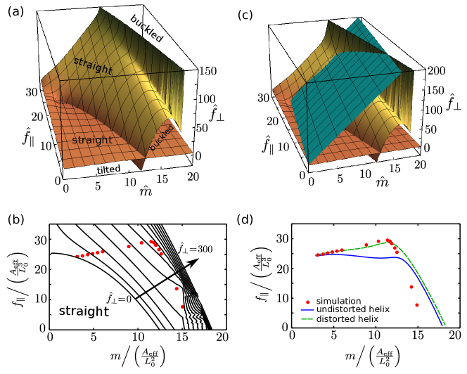
Figure 9: (a) Manifold of bifurcation points in the parameter space $(\hat{m},\hat{f}_{\parallel},\hat{f}_{\perp})$. To each parameter triple belongs a specific value of the precession frequency $\hat{\chi}$. (b) Buckling curves $f_{\parallel}(m)$ for different values of the perpendicular force ranging from $\hat{f}_{\perp}=0$ in steps of 25 to 300. The red dots are the critical forces and torques from fig. 7(b). (c) The plane pictures relation (31) between $f_{\parallel}$, $f_{\perp}$, and $m$ for the helical rod with constant friction coefficients. Intersecting it with the manifold of bifurcation points gives the buckling curves in (d). Full blue line: for constant friction coefficients of the undistorted helix, dashed green line: torque-dependent friction coefficients.

Figure 9(a) plots the manifold of bifurcation points. To each parameter triple $(\hat{m},\hat{f}_{\parallel},\hat{f}_{\perp})$ belongs a specific value of the precession frequency $\hat{\chi}$ which we do not discuss further here. At positive $\hat{f}_{\perp}$ and for small $\hat{m}$ and $\hat{f}_{\parallel}$ the straight configuration of the helical rod is stable. If we change the sign of $\hat{f}_{\perp}$, a bifurcation occurs which we interpret as an instability of the straight rod when it reorients towards the perpendicular configuration. We saw this instability in our simulations when we reversed the driving torque as discussed in sects. 3.1.1 and 3.2. Here we keep the direction of the torque but reverse the sign of the velocity $v$ and thereby the sign of $\hat{f}_{\perp}$ in Eq. (27) by reversing the chirality of the rod. The main result is the surface in dark yellow that belongs to the first buckling transition observed in our simulations, so at large $\hat{m}$ the rod is buckled. Finally, at $\hat{f}_{\perp}\approx 0$ and large $\hat{m}$ a transition between two different configurations of the buckled rod occurs. An interesting feature is the ridge in the bifurcation surface. However, we could not determine any dramatic changes in the buckling of the helical rod close to this ridge.

Figure 9(b) shows buckling curves $\hat{f}_{\parallel}(\hat{m})$ for different values of the perpendicular force ranging from $\hat{f}_{\perp}=0$ in steps of 25 to 300. At $\hat{f}_{\perp}=0$ the typical parabolic curve of Eq. (1) occurs. At constant but small value of $m$, the critical force $f_{\parallel}$ increases strongly with increasing $\hat{f}_{\perp}$. Likewise, one needs large forces $\hat{f}_{\perp}$ to stabilize the straight helical rod at high torques. The red dots are the critical forces and torques from fig. 7(b) determined in our simulations. We plot them in reduced units where we calculate $A_{\text{eff}}$ from Eq. (17). Note that the buckling curves develop a shoulder at $\hat{m}$ around 15 for increasing $\hat{f}_{\perp}$ due to the ridge in the manifold of bifurcation points in fig. 9(a). The two simulation points at large $m$ are close to this ridge. We speculate that the transition from a supercritical bifurcation observed in our simulations at low $m$ to a subcritical bifurcation at large $m$ is connected to the existence of this ridge.

In the rotating helical filament or helical rod, the forces $f_{\parallel}$ and $f_{\perp}$ and the torque $m$ are related to each other by Eqs. (22) and (27). Eliminating velocity $v$ and angular frequency $\omega$, one arrives at

$$f_{\perp} =\frac{a_{\perp}}{a_{\parallel}b_{\parallel}-c_{\parallel}^{2}}\left(b_{\parallel}f_{\parallel}-c_{\parallel}m\right).$$ (31)

We give the friction coefficients in terms of the helical parameters in appendix A. Relation (31) defines a plane in the parameter space $(\hat{m},\hat{f}_{\parallel},\hat{f}_{\perp})$ which we intersect in fig. 9(c) with the manifold of bifurcation points. The resulting bifurcation curve is then plotted in fig. 9(d) as full blue line. At low $m$ we have a remarkable quantitative agreement with our simulations (red dots) but we miss the slight increase of the critical force $f_{\parallel}$. We already discussed that the location of the buckling transition is sensitive to small variations in the parameters. We also mentioned in the discussion of the simulation results that close to the buckling transition the helical filament is slightly deformed. In Ref. Vogel2010 we calculated the effective spring constant $A/(R^{2}L)$ for the helical filament. It gives a relative compression of the filament of about $2\%$ for critical forces of $1\mathrm{p}\mathrm{N}$ at the buckling transition, which is negligible. On the other hand, we apply a torque along the helical axis. As a result, one end of the helix twists against the other end by an angle $\Delta\phi/L=M/A$, where we set $A=C$ Love1944 . One end of the helical filament is free, so the twist increases linearly from the free end to the other and the average value is $M/(2A)$. Due to the twisting, the radius of the helix changes. One can show that for the average twist angle $M/(2A)$ the inverse radius $R^{-1}$ changes to $R^{-1}+(\cos\alpha)^{-1}M/(2A)$. Here we keep the pitch angle $\alpha$ constant, which is confirmed by our simulations. The helical radius directly influences the friction coefficients $b_{\|}$ and $c_{\|}$ in Eq. (31) [see Eqs. (38) and (39b) in appendix A] and Eq. (31) becomes a nonlinear function in $m=M/L_{0}$. Intersecting it with the bifurcation manifold gives the green curve in fig. 9(d) which nicely reproduces the critical force-torque relation for $\hat{m}<10$. Our theory also gives the strong decrease of the critical force $f_{\|}$ at large $m$. However, in the effective model the bifurcation is shifted to larger torque values. This might be related to the ridge in the manifold of bifurcation points. Nevertheless, considering the fact that we approximate the helical filament by a rigid rod whose helicity comes in through the friction coefficients, we obtain a very good agreement with our simulations.

5 Summary and conclusions

Bacteria move forward by rotating a bundle of helical flagella which creates a thrust force that pushes against the cell body. In this article we have modeled a single flagellum based on the discretized version of Kirchhoff’s elastic-rod theory and developed a coarse-grained approach for driving the helical filament by a motor torque. When increasing the motor torque, the thrust force reveals a supercritical Hopf bifurcation due to buckling of the helical filament. When the torque is further increased, a second buckling instability occurs. The Hopf bifurcation is also visible when we attach the flagellum to a spherical particle, which mimics the cell body, so that the whole model bacterium moves forward. Via the size of the cell body we can tune the thrust force pushing against the cell body and the critical torque for buckling changes. This results in a characteristic diagram critical force versus torque for the buckling transition [fig. 7(b)].

We have developed a theory for the observed buckling transition by approximating the helical filament by a helical rod with an effective bending rigidity and the characteristic rotation-translation coupling. The basic picture is that the filament buckles under the frictional forces and torques that act along the filament when the filament rotates. For large friction of the load particle, when its size is comparable to a bacterial cell body, buckling is mostly due to the thrust force created along the filament and similar to a rod that buckles under its own weight. In the limit of small friction of the load particle, the critical thrust force tends to zero and buckling is mostly driven by the frictional torque acting along the filament. However, our modeling reveals that subtle details of the specific problem are important. One has to take into account the precession of the buckled filament about the applied torque and, in particular, a perpendicular frictional force due to the motion of the model bacterium that stabilizes the filament against buckling. Finally, taking into account the small deformation of the rotating helical filament, we are able to obtain a quantitative agreement with the simulated graph, critical force versus torque, in the biologically relevant regime.

To further illustrate the biological relevance of the observed buckling transition, we first summarize a few experimental values. Hotani gives the motor torque for observing a polymorphic transition of the flagellum at around $1.1\mathrm{p}\mathrm{N}\mathrm{\SIUnitSymbolMicro}\mathrm{m}$ Hotani1982 , whereas Darnton et al. mention a mean torque acting on a flagellum of about $1.4\mathrm{p}\mathrm{N}\mathrm{\SIUnitSymbolMicro}\mathrm{m}$ Darnton2007a . These values agree with the torques where we observe buckling for realistic cell body sizes (see fig. 7). Reference Darnton2007a also mentions the relative stiffness of the helical filament so that it hardly deforms under rotation which agrees with our simulations. Finally, thrust forces created by the bundle are given as $0.41\pm 0.23\mathrm{p}\mathrm{N}$ Darnton2007a or $0.5\mathrm{p}\mathrm{N}$ Chattopadhyay2006 . This agrees with an estimate $F=6\pi\eta av\approx 0.6\mathrm{p}\mathrm{N}$ where we take the radius of the load particle as $a=1\mathrm{\SIUnitSymbolMicro}\mathrm{m}$ and use the swimming velocity $v=30\mathrm{\SIUnitSymbolMicro}\mathrm{m}/\mathrm{s}$. All these values are close but below the simulated values $F_{\mathrm{c1}}\approx 1\mathrm{p}\mathrm{N}$ for real cell sizes. However, we note that $F_{\mathrm{c1}}$ scales as $A_{\mathrm{eff}}/L_{0}^{2}$, as our analytic model shows, and thereby depends on the explicit choice of the bending ($A$) and torsional ($C$) rigidities. We have chosen particular values for them and also set $A=C$ in our simulations. So $F_{\mathrm{c1}}$ will vary with the actual parameters.

It is clear that swimming bacteria should avoid buckling for efficient locomotion. However, they cannot simply increase bending rigidity $A$ since a certain flexibility is necessary during polymorphic transformations or when a bundle forms. Reference Turner2000 shows pictures where single flagella are in a bent conformation similar to the buckled state in our simulations. This might be a hint that flagella naturally buckle under their own thrust. In peritrichous bacteria such as E.Coli and Salmonella, several flagella form a bundle which then has larger bending stiffness and therefore buckling is not observed.

Monotrichous bacteria only use a single flagellum. Their conformation differs in pitch and radius from the flagella of peritrichous bacteria Fujii2008 . A detailed analysis shows that their swimming efficiency is reduced due to a smaller pitch angle with $\sin\alpha\approx 0.75$ Spagnolie2011 . This increases the critical force $F_{cr}\propto 1/\sin\alpha$ by about $10\%$ compared to peritrichous bacteria and might be an adaption of the monotrichous bacteria to enhance the stability of their single flagellum.

We also showed that a pulling flagellum is not stably aligned along the applied torque. So most bacteria use their flagella to push themselves through the fluid. Nevertheless, there are some marine bacteria that use a back-and-forth rather than a run-and-tumble strategy for chemotaxis. They live in a turbulent aqueous environment in the ocean where they experience large shear gradients on the micron scale Luchsinger1999 . Simulations in Ref. Luchsinger1999 show that in addition to the shear-driven reorientation of the bacterium there must be further contributions to the reorientation. Besides rotational diffusion this could also be the unstable orientation of the rotating filament when it pulls the cell body. Recent experiments on the back-and-forth motion of marine bacteria Vibrio alginolyticus directly show this reorientation of the flagellum Xie2011 .

We close with this comment and hope that our work initiates a more careful search for the buckling transition in bacterial flagella.

Appendix A Summary of resistive force theory for a helix

At low Reynolds number the force $\boldsymbol{F}$ and torque $\boldsymbol{M}$ acting on a particle of arbitrary shape are linearly related to its translational and rotational velocities Happel1983 ,

$$\begin{pmatrix}\boldsymbol{F}\\ \boldsymbol{M}\end{pmatrix} =\begin{pmatrix}\boldsymbol{\sf A}&\boldsymbol{\sf C}\\ \boldsymbol{\sf C}^{\mathtt{T}}&\boldsymbol{\sf B}\end{pmatrix}\begin{pmatrix}\boldsymbol{v}\\ \boldsymbol{\omega}\end{pmatrix}.$$ (32)

The translational friction tensor $\boldsymbol{\sf A}$, the rotational friction tensor $\boldsymbol{\sf B}$, and the coupling tensor $\boldsymbol{\sf C}$ are determined by the shape of the particle. Note that the rotational friction tensor $\boldsymbol{\sf B}$ and the coupling tensor $\boldsymbol{\sf C}$ depend on the choice of the origin of the coordinate system whereas the translational friction tensor $\boldsymbol{\sf A}$ is unique.

In a moving helical filament, different parts interact via hydrodynamic interactions. Nevertheless, using slender-body theory, Lighthill demonstrated that one can describe the hydrodynamic friction of the filament with the help of resistive force theory Lighthill1976 ; Childress1981 . In this theory one introduces local friction coefficients per unit length parallel ($\gamma_{\parallel}$) and perpendicular ($\gamma_{\perp}$) to the tangent vector of the filament. Lighthill adjusted the coefficients for the helical filament to Lighthill1976

$$\gamma_{\parallel} =\frac{2\pi\eta}{\ln(2q/r)}\enspace\mathrm{and}\enspace\gamma_{\perp}=\frac{4\pi\eta}{\ln(2q/r)+1/2}.$$ (33)

Here $\eta$ is the shear viscosity, $r=0.02\mathrm{\SIUnitSymbolMicro}\mathrm{m}$ the cross-sectional radius of the bacterial flagellum, and $q$ a characteristic length, for which Lighthill derived $q=0.09\Lambda$, where $\Lambda=2\pi R/\cos\alpha$ is the filament length of one helical turn.

In a helical filament with translational velocity $\boldsymbol{v}$ and angular frequency $\boldsymbol{\omega}$ each segment moves with a velocity $\boldsymbol{v}+\boldsymbol{\omega}\times\boldsymbol{r}$, where $\boldsymbol{r}$ is the position vector from a point on the helical axis to the segment. The force and torque densities to initiate such a motion are

$$\boldsymbol{f} =\left(\gamma_{\parallel}\boldsymbol{\sf P}_{\parallel}+\gamma_{\perp}\boldsymbol{\sf P}_{\perp}\right)\cdot(\boldsymbol{v}+\boldsymbol{\omega}\times\boldsymbol{r})$$ (34)

$$\boldsymbol{m} =\boldsymbol{r}\times\boldsymbol{f},$$ (35)

where we use the projectors on the local tangent vector $\boldsymbol{e}_{3}$ and the space perpendicular to it,

$$\boldsymbol{\sf P}_{\parallel} =\boldsymbol{e}_{3}\otimes\boldsymbol{e}_{3},\quad\text{and} \boldsymbol{\sf P}_{\perp} =\boldsymbol{\sf 1}-\boldsymbol{e}_{3}\otimes\boldsymbol{e}_{3}.$$ (36)

Integrating force and torque densities along the helical filament with position vector

$$\boldsymbol{r}(s)=\left(R\cos\left(\frac{\cos\alpha}{R}s\right),R\sin\left(\frac{\cos\alpha}{R}s\right),\sin\alpha s\right)^{\mathtt{T}},$$ (37)

gives Eq. (32). For comparing theory and simulation in sect. 3, we calculated the integrals using the computational software program “Mathematica”. In particular, we took into account that the helical filament in the simulations does not consists of an integral number of helical turns and that the rotational axis is shifted against the helical axis. In our analytical theory for the buckling transition in sect. 4, we used friction coefficients calculated for a full helical turn with $L=2\pi R/\cos\alpha$. The relevant coefficients become

$$A_{\perp} =L\gamma_{\perp}\left(1+\frac{\delta}{2}\cos^{2}\alpha\right)$$ (38a)

$$A_{\parallel} =L\gamma_{\perp}\left(1+\delta\sin^{2}\alpha\right)$$ (38b)

$$B_{\parallel} =L\gamma_{\perp}R^{2}\left(1+\delta(1-\sin^{2}\alpha)\right)$$ (38c)

$$C_{\parallel} =L\gamma_{\perp}R\delta\sin\alpha\cos\alpha,$$ (38d)

where we use $\delta=\frac{\gamma_{\parallel}-\gamma_{\perp}}{\gamma_{\perp}}$ to characterize the anisotropy in the local friction coefficients. Note that $A_{\parallel}$ also holds for arbitrary filament lengths when $L$ is not an integer of a full helical turn. For all other coefficients one obtains corrections of the form $\sin\left(\frac{\cos\alpha}{R}L\right)$ that vanish in the limit $L\to\infty$.

The effective friction coefficients for the helical rod used in Sec. 4 follow by dividing the friction coefficients of Eqs. (38) by the rod length $L_{0}=L\sin\alpha$:

$$a_{\perp} =A_{\perp}/L_{0}, a_{\parallel} =A_{\parallel}/L_{0},$$ (39a)

$$b_{\parallel} =B_{\parallel}/L_{0}, c_{\parallel} =C_{\parallel}/L_{0},$$ (39b)

Appendix B Rotational motion of a rigid helix

Starting from Eq.  (32) we set $\boldsymbol{v}=0$ and concentrate on the rotational motion due to a constant external torque $\boldsymbol{M}$ with the relevant equation

$$\boldsymbol{M} =\boldsymbol{\sf B}\boldsymbol{\omega}.$$ (40)

The rotational friction tensor $\boldsymbol{\sf B}$ is symmetric. In the following we use its frame of eigenvectors $\{\boldsymbol{e}_{1},\boldsymbol{e}_{2},\boldsymbol{e}_{3}\}$ and the eigenvalues $B_{1}$, $B_{2}$, and $B_{3}$. We differentiate Eq. (40) with respect to time $t$, use $\partial_{t}\boldsymbol{e}_{i}=\omega\times\boldsymbol{e}_{i}$, and obtain in the eigenframe of $\boldsymbol{\sf B}$,

$$B_{1}\partial_{t}\omega_{1} =(B_{2}-B_{3})\omega_{2}\omega_{3},$$ (41)

$$B_{2}\partial_{t}\omega_{2} =(B_{3}-B_{1})\omega_{1}\omega_{3},$$ (42)

$$B_{3}\partial_{t}\omega_{3} =(B_{1}-B_{2})\omega_{1}\omega_{2}.$$ (43)

These equations are the same as the Euler equations for a rigid body with an inertia tensor $\boldsymbol{\sf B}$ and without friction. The external torque is zero so that angular momentum is conserved. Following this analogy and according to Eq. (40), the constant external torque in our case corresponds to the angular momentum of the rigid body, and the dissipated energy $P=\boldsymbol{M}\cdot\boldsymbol{\omega}$ to the rotational kinetic energy. Hence, besides the square of the applied torque $M^{2}=\sum_{i}B_{i}^{2}\omega_{i}^{2}$ also the dissipated energy $P=\sum_{i}B_{i}\omega_{i}^{2}$ is a conserved quantity and the trajectory of $\boldsymbol{\omega}$ follows from the intersection of two ellipsoids as illustrated in fig. 10(a). In particular, if two of the friction coefficients $B_{i}$ are equal, the angular velocity $\boldsymbol{\omega}$ precesses in real space on a cone about the direction of the torque Landau1976 ; Arnold1978 .

We already calculated one component of the rotational friction tensor $\boldsymbol{\sf B}$ of a helix with filament length $L$ in the previous section. In general, for a long slender helix like the normal form of the bacterial flagellum two eigenvalues of $\boldsymbol{\sf B}$ are equal to a good approximation, $B_{1}\approx B_{2}\propto L^{3}$. The third small friction coefficient $B_{3}\propto L$ belongs to the principal axis, which is parallel to the helical axis, again to a good approximation. Hence, a rigid helical filament precesses about the applied torque [fig. 10(b)] and does not align parallel to the torque as observed in our simulations.

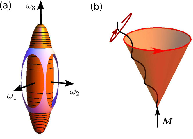
Figure 10: (a) The constant applied torque and the dissipated energy define two ellipsoids (red and blue) in the body fixed frame of a rigid helix. The intersection gives the path of the angular velocity $\boldsymbol{\omega}$. For a long slender helix two directions are degenerate and the trajectories are circles. (b) In the lab frame the helix rotates about its axis which precesses about the applied torque $\boldsymbol{M}$.

Appendix C Effective bending rigidity of a helix

We aim at replacing the helical filament by a rod with an effective bending rigidity $A_{\text{eff}}$. Our strategy is to apply a small constant torque perpendicular to the helical axis, rewrite the total elastic energy as a function of the torque, and compare this result with the case of a simple rod to obtain $A_{\text{eff}}$. To bend a simple rod with a constant curvature $\Omega$, one needs the bending energy $\mathcal{F}=\frac{1}{2}A_{\text{eff}}\Omega^{2}L_{0}$. Using the torque $M=A_{\text{eff}}\Omega$ [see, for example, Eq. (20)), we obtain

$$\mathcal{F} =\frac{1}{2}\frac{M^{2}}{A_{\text{eff}}}L_{0}.$$ (44)

Now we calculate the corresponding elastic energy for the helical filament. We apply a constant torque $\boldsymbol{M}=M\boldsymbol{e}_{x}$ perpendicular to the helical axis $\boldsymbol{e}_{z}$ and replace in Kirchhoff’s energy density (4) the components of the angular strain vector $\boldsymbol{\Omega}$ by the components of the torque $\boldsymbol{M}=A\Omega_{1}\boldsymbol{e}_{1}+A(\Omega_{2}-\kappa)\boldsymbol{e}_{2}+C(\Omega_{3}-\tau)\boldsymbol{e}_{3}$:

$$f_{\text{cl}} =\frac{1}{2}\left(\frac{M_{1}^{2}}{A}+\frac{M_{2}^{2}}{A}+\frac{M_{3}^{2}}{C}\right).$$ (45)

Note that the components of the applied torque, $M_{i}=M\boldsymbol{e}_{x}\cdot\boldsymbol{e}_{i}$, depend on the local material frame $\{\boldsymbol{e}_{1},\boldsymbol{e}_{2},\boldsymbol{e}_{3}\}$ of the helical filament. In leading order in $M$, we calculate the components $M_{i}$ for the undeformed helical filament of Eq. (37) using the Frenet frame and integrate Eq. (45) along the filament:

$${\mathcal{F}} =\frac{M^{2}L}{4}\left[\frac{1}{A}+\frac{\sin^{2}\alpha}{A}+\frac{\cos^{2}\alpha}{C}+O\left(\frac{\sin 2kL}{2kL}\right)\right],$$ (46)

where we used $k=\cos\alpha/R$. We compare this result with Eq. (44) and introduce the helix height $L_{0}=L\sin\alpha$ in order to identify the effective bending rigidity

$$\frac{1}{A_{\text{eff}}} =\frac{1}{2}\frac{1}{\sin\alpha}\frac{1}{A}\left(1+\sin^{2}\alpha+\frac{A}{C}\cos^{2}\alpha\right).$$ (47)

To verify the applicability of the effective bending rigidity, we study in detail the reorientation rate $\lambda$ of the fixed flagellum, when the thrust force pulls at it (see sect. 3.1.2). Our claim is that the reorientation rate depends on the bending of the helical filament as a whole and thus $A_{\text{eff}}$ should be the relevant parameter. We therefore determined $\lambda$ as a function of the motor torque $M$ for different values of the bending rigidity $A$ and the torsional rigidity $C$ (see fig. 11). In addition to the helical geometry of peritrichous bacteria used in this paper, we also considered the flagellum of monotrichous bacteria, which has different helical parameters: $\kappa_{0}=2.2\mathrm{/}\mathrm{\SIUnitSymbolMicro}\mathrm{m}$ and $\tau_{0}=2.5\mathrm{/}\mathrm{\SIUnitSymbolMicro}\mathrm{m}$ Fujii2008 . Dimensional analysis suggests to rescale the torque $M$ by the characteristic bending moment $A_{\text{eff}}/L_{0}$ as in Sect. 4 and the reorientation rate $\lambda$ by $A_{\text{eff}}/(\frac{1}{3}L_{0}^{3}A_{\perp})$, where $A_{\perp}$ is the friction coefficient introduced in Eq. (38a). With such a rescaling all different curves for the reorientation rate fall onto a common master curve in fig. 11. The effective bending rigidity $A_{\text{eff}}$ is therefore the right parameter in an effective description of the helical filament.

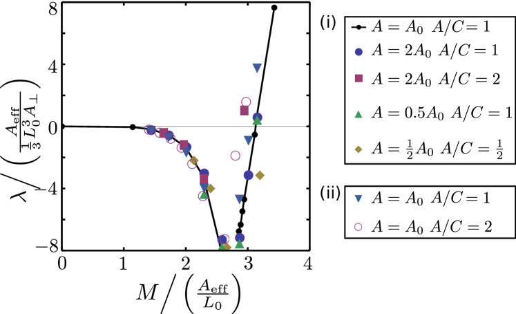
Figure 11: Reorientation rate $\lambda$ as a function of motor torque $M$ for different elastic constants, where $A_{0}=3.5\mathrm{p}\mathrm{N}\mathrm{\SIUnitSymbolMicro}\mathrm{m}^{2}$ is the bending rigidity used in this article. Two helical geometries of the flagellum are considered: (i) for peritrichous bacteria used in this article and (ii) for monotrichous bacteria.

References

- (1) H. C. Berg, E. coli in Motion, Springer Verlag, New York (2004).
- (2) N. Darnton, L. Turner, K. Breuer, H. C. Berg, Biophys J, 86, 1863–1870 (2004).
- (3) W. R. Hesse, L. Luo, G. Zhang, R. Mulero, J. Cho, M. J. Kim, Materials Science and Engineering C 29, 2282 - 2286 (2009).
- (4) L. Zhang, J. J. bbott, L. Dong, B. E. Kratochvil, D. Bell, B. J. Nelson, Appl. Phys. Lett. 94, 064107 (2009).
- (5) N. C. Darnton, L. Turner, S. Rojevsky, H. C. Berg, J Bacteriol 189, 1756-1764 (2007).
- (6) L. Turner, W. S. Ryu, H. C. Berg, J. Bacteriol. 182, 2793-2801 (2000). See also http://webmac.rowland.org/labs/bacteria/movies_ecoli.html
- (7) M. Kim, J. C. Bird, A. J. V. Parys, K. S. Breuer, T.R. Powers, PNAS, 100, 15481-15485 (2003).
- (8) M. Kim, T. R. Powers, Phys Rev E, 69, 061910 (2004).
- (9) M. Reichert, H. Stark, EPJE, 17, 493-500 (2005).
- (10) P. J. A. Janssen, M. D. Graham, Phys. Rev. E, 84, 011910 (2011).
- (11) S. Asakura, Adv. Biophys. 1, 99 (1970).
- (12) C. Calladine, Nature 255, 121 (1975).
- (13) R. M. Macnab and M. K. Ornston, J. Mol. Biol. 112, 1 (1977).
- (14) H. Hotani, J. Mol. Bio., 156, 791 - 806 (1982).
- (15) E. Hasegawa, R. Kamiya and S. Asakura, J. Mol. Biol. 160, 609 (1982).
- (16) R. E. Goldstein, A. Goriely, G. Huber, and C. W. Wolgemuth, Phys. Rev. Lett. 84, 1631 (2000).
- (17) S. V. Srigiriraju and T. R. Powers, Phys. Rev. Lett. 94, 248101 (2005).
- (18) N. C. Darnton and H. C. Berg, Biophys. J. 92, 2230 (2007).
- (19) H. Wada and R. R. Netz, Europhys. Lett. 82, 28001 (2008).
- (20) C. Speier, R. Vogel, H. Stark, Phys. Biol. , 8, 046009 (2011)
- (21) M. Schmitt, H. Stark, EPL (Europhysics Letters), 96, 28001 (2011).
- (22) R. Vogel and H. Stark, Eur. Phys. J. E 33, 259–271 (2010).
- (23) A. E. H. Love, A Treatise on the Mathematical Theory of Elasticity (New York Dover Publications, 1944).
- (24) C. W. Wolgemuth, T. R. Powers, and R. E. Goldstein, Phys. Rev. Lett., 84, 1623 (2000).
- (25) H. Wada, R. R. Netz, Europhysics Letters 75, 645-651 (2006).
- (26) M. Manghi, X. Schlagberger, R. R. Netz, Physical Review Letters 96, 068101 (2006).
- (27) L. Landau and E. Lifshitz, Theory of Elasticity (Pergamon Press, 1986).
- (28) E.M. Purcell, Am. J. Phys 45, 3 (1977).
- (29) S. Chattopadhyay, R. Moldovan, C. Yeung, and X. L. Wu, PNAS 103, 13712 (2006).
- (30) S. Chattopadhyay and X. L. Wu, Biophys. J. 96, 2023 (2009).
- (31) M. Reichert, Ph.D. thesis, University Konstanz (2006), http://nbn-resolving.de/urn:nbn:de:bsz:352-opus- 19302.
- (32) G. Chirico and J. Langowski, Biopolymers 34, 415 (1994).
- (33) H. Wada and R. R. Netz, Europhys. Lett. 77, 68001 (2007).
- (34) H. Wada and R. R. Netz, Phys. Rev. Lett. 99, 108102 (2007).
- (35) C. J. Jones, R. M. Macnab, H. Okino, S. -I. Aizawa, Journal of Molecular Biology 212, 377 - 387 (1990).
- (36) K. Kobayashi, T. Saitoh, D. S. H. Shah, K. Ohnishi, I. G. Goodfellow, R. E. Sockett, S. -I. Aizawa, J. Bacteriol. 185, 5295-5300 (2003).
- (37) F. A. Samatey, H. Matsunami, K. Imada, S. Nagashima, T. R. Shaikh, D. R. Thomas, J. Z. Chen, D. J. DeRosier, A. Kitao, K. Namba, Nature 431, 10621068 (2004).
- (38) T. R. Shaikh, D. R. Thomas, J. Z. Chen, F. A. Samatey, H. Matsunami, K. Imada, K. Namba, D. J. Derosier, Proc Natl Acad Sci 102, 1023-1028 (2005).
- (39) T. Furuta and F. A. Samatey, H. Matsunami, K. Imada, K. Namba and A. Kitao, J. Struct. Biology, 157, 481 (2007).
- (40) J. Lighthill, SIAM Rev. 18, 161 (1976).
- (41) S. Childress, Mechanics of swimming and flying. (Cambridge University Press, 1981).
- (42) L. Landau and E. Lifshitz, Mechanics (Pergamon Press, 1976).
- (43) V. I. Arnold, Mathematical Methods of Classical Mechanics (Springer-Verlag, 1978).
- (44) J. Haringx, Proc. Ned. Akad. Wet., 45, 533-539 & 650-654 (1942).
- (45) J. Haringx, Philips Research Reports, 3, 401-449 (1948).
- (46) C. Biezeno & R. Grammel, Technische Dynamik (Springer, 1939).
- (47) D. Karpeev, I. S. Aranson, L. S. Tsimring, H. G. Kaper, Interactions of semiflexible filaments and molecular motors. Phys Rev E, 76, 051905 (2007).
- (48) M. Fujii, S. Shibata, S. -I. Aizawa, Journal of Molecular Biology 379, 273 - 283 (2008).
- (49) S. E. Spagnolie, E. Lauga, Phys. Rev. Lett. 106, 058103 (2011).
- (50) R. H. Luchsinger, B. Bergersen, J. G. Mitchell, Bacterial swimming strategies and turbulence. Biophys J, 77, 2377-2386 (1999).
- (51) L. Xie, T. Altindal, S. Chattopadhyay, X. -L. Wu, Proc Natl Acad Sci, 108, 2246-2251 (2011).
- (52) J. Happel & H. Brenner, Low Reynolds Number Hydrodynamics (Springer, 1983).
- (53) C. Brennen and H. Winet, Annu. Rev. Fluid Mech. 9, 339 (1977).