Interplay of quantum stochastic and dynamical maps to discern Markovian and non-Markovian transitions

Abstract

It is known that the dynamical evolution of a system, from an initial tensor product state of system and environment, to any two later times, $t_{1},t_{2}\ (t_{2}>t_{1})$, are both completely positive (CP) but in the intermediate times between $t_{1}$ and $t_{2}$ it need not be CP. This reveals the key to the Markov (if CP) and nonMarkov (if it is not CP) avataras of the intermediate dynamics. This is brought out here in terms of the quantum stochastic map $A$ and the associated dynamical map $B$ – without resorting to master equation approaches. We investigate these features with four examples which have entirely different physical origins (i) a two qubit Werner state map with time dependent noise parameter (ii) Phenomenological model of a recent optical experiment (Nature Physics, 7, 931 (2011)) on the open system evolution of photon polarization. (iii) Hamiltonian dynamics of a qubit coupled to a bath of $N$ qubits and (iv) two qubit unitary dynamics of Jordan et. al. (Phys. Rev. A70, 052110 (2004) with initial product states of qubits. In all these models, it is shown that the positivity/negativity of the eigenvalues of intermediate time dynamical $B$ map determines the Markov/non-Markov nature of the dynamics.

I Introduction

Understanding the basic nature of dynamical evolution of a quantum system, which interacts with an inaccessible environment, attracts growing importance in recent years Breuer ; Alicki . This offers the key to achieve control over quantum systems – towards their applications in the emerging field of quantum computation and communication Niel . While the overall system-environment state evolves unitarily, the dynamics governing the system is described by a completely positive (CP), trace preserving map ECGS1 ; Choi ; ji .

Markov approximation holds when the future dynamics depends only on the present state – and not on the history of the system i.e., memory effects are negligible. The corresponding Markov dynamical map constitutes a trace preserving, CP, continuous one-parameter quantum semi-group Lindblad ; GKS . Markov dynamics governing the evolution of the system density matrix is conventionally described by Lindblad-Gorini-Kossakowski-Sudarshan (LGKS) master equation Lindblad ; GKS $\frac{d\rho}{dt}={\cal L}\rho$, where ${\cal L}$ is the time-independent Lindbladian operator generating the underlying quantum Markov semi-group. Generalized Markov processes are formulated in terms of time-dependent Lindblad generators and the associated trace preserving CP dynamical map is a two-parameter divisible map div ; RHP , which too corresponds to memory-less Markovian evolution.

Not completely positive (NCP) maps do make their presence felt in the open-system dynamics obtained from the joint unitary evolution – if the system and environment are in an initially quantum correlated state Jordan ; Rosario ; Anil ; Kavan . In such cases, the open-system evolution turns out to be non-Markovian AKRUS . However, the source of such non-Markovianity could not be attributed entirely to either initial system-environment correlations or their dynamical interaction or both. This issue gets refined if initial global state is in the tensor product form, in which case the sole cause of Markovianity/non-Markovianity could be attributed to dynamics alone. It is known that the time evolution of a subsystem from an initial tensor product form to two different later times, $t_{1},t_{2}\ (t_{2}>t_{1})$, are both CP. However the dynamics in the intermediate time steps between $t_{1}$ and $t_{2}$ need not be CP. The quantum stochastic $A$ and dynamical $B$ maps – first introduced as a quantum extension of classical stochastic dynamics – by Sudarshan, Mathews, Rau and Jordan (SMRJ) ECGS1 nearly five decades ago, offer an elegant approach to explore Markovian/non-Markovian nature of open system evolution. The interplay of $A$ and $B$ maps at intermediate times, to bring out the Markov or non-Markov avataras of open system evolution, is established in this paper.

To place these ideas succinctly, there are three basic aspects in open system quantum dynamics: (1) nature of dynamical interaction between the system and its environment, (2) role of initial correlations in system-environment state and (3) nature of dynamics at intermediate times. Last few years have witnessed intense efforts towards understanding these Jordan ; Rosario ; Anil ; Kavan ; div ; RHP ; NM ; AKRUR ; AKRUS ; BLP ; haikka ; kos ; Hou . The third issue is the focus here to discern the Markov/non-Markov nature of dynamics in terms of intermediate time $A$ and $B$ maps.

The contents are organized as follows: In Sec. II some basic concepts ECGS1 on $A$ and $B$ maps are given. The emergence of CP/NCP maps, at intermediate times, under open system dynamics is discussed in Sec. III. Sec.IV is devoted to a powerful link (brought out by Jamilkowski isomorphism) between the $B$ map and the dynamical state. Some illustrative examples of dynamical $B$ map to investigate the CP/NCP nature of dynamics at intermediate times are discussed in Sec. V. The examples are chosen from different origins: one based entirely from the general considerations of Jamiolkowski isomorphism; second one on the recent all-optical open system experiment to drive Markovian to non-Markovian transitions; the other two examples are based on open system Hamiltonian dynamics. In all these four examples, no master equation is employed in the deduction of Markov to non-Markov transitions – but the CP/NCP nature of the intermediate dynamical map (via the sign of the eigenvalue of the $B$ map) has been invoked. Sec. VI has some concluding remarks.

II Preliminary ideas on dynamical $A$ and $B$ maps

The stochastic $A$ and dynamical $B$ maps ECGS1 transform the initial system density matrix $\rho_{S}(t_{0})$ to final density matrix $\rho_{S}(t)$ via,

$$\left[\rho_{S}(t)\right]_{b_{1}b_{2}} = \sum_{a_{1},a_{2}}\left[A(t,t_{0})\right]_{b_{1}b_{2};a_{1}a_{2}}\,\left[\rho_{S}(t_{0})\right]_{a_{1}a_{2}},$$ (1)

$$\left[\rho_{S}(t)\right]_{b_{1}b_{2}} = \sum_{a_{1},a_{2}}\left[B(t,t_{0})\right]_{b_{1}a_{1};b_{2}a_{2}}\,\left[\rho_{S}(t_{0})\right]_{a_{1}a_{2}},$$

$$\ \ \ \ \ a_{1},a_{2},b_{1},b_{2}=1,2,\ldots,d$$

where the realligned matrix $B$ is defined by,

$$B_{b_{1}a_{1};b_{2}a_{2}}=A_{b_{1}b_{2};a_{1}a_{2}}.$$ (3)

The requirement that the evolved density matrix $\rho_{S}(t)$ has unit trace and is Hermitian, positive semi-definite places the following conditions on $A$ and $B$ ECGS1 :

$${\rm Trace\ preservation}: \ \ \sum_{b_{1}}A_{b_{1}b_{1};a_{1}a_{2}}=\delta_{a_{1}a_{2}},$$

$$\ \ \sum_{b_{1}}B_{b_{1}a_{1};b_{1}a_{2}}=\delta_{a_{1}a_{2}},$$

$${\rm Hermiticity}:\ \ \ \ \ A_{b_{1}b_{2};a_{1}a_{2}}=A^{*}_{b_{2}b_{1};a_{2}a_{1}},$$ (4)

$$\ \ B_{b_{1}a_{1};b_{2}a_{2}}=B^{*}_{b_{2}a_{2};b_{1}a_{1}}$$

$${\rm Positivity}:\ \ \ \ \ \sum_{a_{1},a_{2},b_{1},b_{2}}\,x^{*}_{b_{1}}\,x_{b_{2}}\,A_{b_{1}b_{2};a_{1}a_{2}}\,y_{a_{1}}\,y_{a_{2}}^{*}\geq 0,$$

$$\ \ \sum_{a_{1},a_{2},b_{1},b_{2}}\,x^{*}_{b_{1}}\,y_{a_{1}}\,B_{b_{1}a_{1};b_{2}a_{2}}\,x_{b_{2}}\,y_{a_{2}}^{*}\geq 0$$

It may be readily identified that the dynamical $B$ map is positive, Hermitian $d^{2}\times d^{2}$ matrix with trace $d$ – corresponding to CP evolution. We would also like to point out here that the composition of two stochastic $A$-maps, $A_{1}\ast A_{2}$ tranforming $\rho_{S}(t_{0})\stackrel{{\scriptstyle A_{1}}}{{\longrightarrow}}\rho_{S}(t_{1})\stackrel{{\scriptstyle A_{2}}}{{\longrightarrow}}\rho_{S}(t_{2})$ is merely a matrix multiplication, whereas it is not so in its $B$-form.

III CP/NCP nature of Intermediate time $A$ and $B$ maps

Let us consider unitary evolution of global system-environment state $\rho_{S}(t_{0})\otimes\rho_{E}(t_{0})$ from an initial time $t_{0}$ to a final time $t_{2}$ – passing through an intermediate instant $t_{1}$ (i.e., $t_{0}<t_{1}<t_{2}$). The $A$-map associated with $t_{0}$ to $t_{1}$ and that between $t_{0}$ to $t_{2}$ are identified as follows:

$${\rm Tr}_{E}\left[U(t_{j},t_{0})\rho_{S}(t_{0})\otimes\rho_{E}(t_{0})U^{\dagger}(t_{j},t_{0})\right]=A(t_{j},t_{0})\,\rho_{S}(t_{0})$$

$$\ \ \ \ \ \ \ \ \ \ =\rho_{S}(t_{j}),\ \ j=1,2.$$ (5)

The stochastic map $A(t_{j},t_{0})$ is completely positive (correspondingly the dynamcal $B(t_{j},t_{0})$ matrix is positive).

In order to identify the intermediate stochastic map $A(t_{2},t_{1})$, we make use of the composition law of unitary evolution $U(t_{2},t_{0})=U(t_{2},t_{1})U(t_{1},t_{0})$:

$${\rm Tr}_{E}\left[U(t_{2},t_{1})\left\{U(t_{1},t_{0})\rho_{S}(t_{0})\otimes\rho_{E}(t_{0})U^{\dagger}(t_{1},t_{0})\right\}U^{\dagger}(t_{2},t_{1})\right]=$$

$$\hskip 72.26999pt\ \ A(t_{2},t_{0})\,\rho_{S}(t_{0}).$$ (6)

However, this does not lead naturally to $A(t_{2},t_{0})=A(t_{2},t_{1})A(t_{1},t_{0})$ for the $A$ map. Invoking Markovian approximation (memory-less reservoir condition note ) $\left\{U(t_{1},t_{0})\rho_{S}(t_{0})\otimes\rho_{E}(t_{0})U^{\dagger}(t_{1},t_{0})\right\}\approx\rho_{S}(t_{1})\otimes\rho_{E}(t_{1})$, the LHS of (III) may be expressed as,

$${\rm Tr}_{E}\left[U(t_{2},t_{1})\rho_{S}(t_{1})\otimes\rho_{E}(t_{1})U^{\dagger}(t_{2},t_{1})\right]=A(t_{2},t_{1})\,\rho_{S}(t_{1}).$$ (7)

Further, substituting $j=1$ in (III) and expressing $\rho_{S}(t_{0})=A^{-1}(t_{1},t_{0})\rho_{S}(t_{1})$ in (III) the intermediate $A$ map $A(t_{2},t_{1})$ is identified:

$$A(t_{2},t_{1})=A(t_{2},t_{0})A^{-1}(t_{1},t_{0}).$$ (8)

In other words, when the environment is passive ( Markovian dynamics), the intermediate $A$-map has the divisible composition as in (8). In such cases $A(t_{1},t_{2})$ is ensured to be CP – otherwise it is NCP, and hence non-Markovian. Correspondingly, the intermediate $B$-map $B(t_{2},t_{1})$ is positive if the dynamics is Markovian; negative eigenvalues of $B(t_{2},t_{1})$ imply non-Markovianity.

IV The $B$ map and the Jamiolkowski Isomorphism

The Jamiolkowski isomorphism ji provides an insight that the $B$-map is directly related to a $d^{2}\times d^{2}$ system-ancilla bipartite density matrix. More specifically, the action of the map $A^{\rm Id}\otimes A$ on the maximally entangled system-ancilla state $|\psi_{\rm ME}\rangle=\frac{1}{\sqrt{d}}\sum_{i=0}^{d-1}|i,i\rangle$ results in the density matrix $\rho_{ab}$ which may be identified to be related to the dynamical $B$ map i.e.,

$$\rho_{ab}=\left[A^{\rm Id}\otimes A\right]|\psi_{\rm ME}\rangle\langle\psi_{\rm ME}|\rightarrow\frac{1}{d}\,B$$ (9)

gives an explicit matrix representation for the $B$-map (Here $A^{\rm Id}$ is the identity A-map, which leaves the ancilla undisturbed).

In detail, we have,

$$\left(\rho_{ab}\right)_{a_{1}b_{1};a_{2}b_{2}} = \sum_{a^{\prime}_{1},a^{\prime}_{2},b^{\prime}_{1},b^{\prime}_{2}}\,\left[A^{\rm Id}\otimes A\right]_{a_{1}b_{1}a_{2}b_{2};a^{\prime}_{1}b^{\prime}_{1}a^{\prime}_{2}b^{\prime}_{2}}\,\left[|\psi_{\rm ME}\rangle\langle\psi_{\rm ME}|\right]_{a_{1}^{\prime}b_{1}^{\prime};a_{2}^{\prime}b_{2}^{\prime}}$$ (10)

$$= \frac{1}{d}\,\sum_{a^{\prime}_{1},a^{\prime}_{2},b^{\prime}_{1},b^{\prime}_{2}}\,\delta_{a_{1},a^{\prime}_{1}}\delta_{a_{2},a^{\prime}_{2}}\,A_{b_{1}b_{2};b_{1}^{\prime}b_{2}^{\prime}}\,\delta_{a_{1}^{\prime},b_{1}^{\prime}}\delta_{a_{2}^{\prime},b_{2}^{\prime}}$$

$$= \frac{1}{d}\,A_{b_{1}b_{2};a_{1}a_{2}}=\frac{1}{d}\,B_{b_{1}a_{1};b_{2}a_{2}},$$

or $\left(\rho_{ba}\right)_{b_{1}a_{1};b_{2}a_{2}}=\frac{1}{d}\,B_{b_{1}a_{1};b_{2}a_{2}}$.

In other words, Jamiolkowski isomorphism maps every completely positive dynamical map $B$ acting on $d$ dimensional space to a positive definite $d^{2}\times d^{2}$ bipartite density matrix $\rho_{ab}$ (See Eq. (10)) – whose partial trace (over the first subsystem – as seen from the trace preservation property on dynamical map $B$ (as in Eq.(II)) is a maximally disordered state. One such set of bipartite $d\times d$ density matrices belong to the class that are invariant under $U\otimes U$ Vol – which constitute the well-known Werner density matrices. One may now identify several toy models of dynamical $B$ maps – including the two qubit Werner state example motivated by the above remark – to investigate the nature of intermediate time dynamics.

In the next section we present specific examples chosen to illustrate the features of intermediate dynamical maps: (i) A toy model map inspired by Jamiolkowski isomorphism – which is not based on any Hamiltonian underpinning. (ii) Recent optical experiment by Liu et. al., Liu on open system evolution of photon polarization to bring out non-Markovianity features is reinterpreted in terms of NCP nature of the intermediate dynamical map. (iii) Intermediate dynamical map in the Hamiltonian evolution of a two-level system coupled to $N$ two-level systems Hou (iv) open system dynamics arising from a two qubit unitary evolution  Jordan .

V Examples

V.1 A toy model dynamical map

The two qubit Werner density matrix is a natural choice for a prototype of dynamical $B$-map – arising from general considerations of the Jamiolkowoski isomorphism:

$$B(t,0)=\frac{[1-p(t)]}{2}\,I_{2}\otimes I_{2}+\frac{p(t)}{2}\,|\Psi^{(-)}\rangle\langle\Psi^{(-)}|$$ (11)

with a time dependent noise parameter $0\leq p(t)\leq 1$, and $|\Psi^{(-)}\rangle=\frac{1}{\sqrt{2}}\left(|0,0\rangle-|1,1\rangle\right)$ is the Bell state. For a dynamical map, time dependence in $p(t)$ occurs due to the underlying Hamiltonian evolution. This state is especially important in that it exhibits both separable and entangled states, as its characteristic parameter $p(t)$ is varied. Its use here as a valid $B$-map is novel in identifying transitions between Markovianity and non-Markovianity in the dynamics as captured from their intermediate time behavior.

On evaluating the corresponding $A$ map $A(t,0)$ (expressed in the standard $\{|0,0\rangle,|0,1\rangle,|1,0\rangle,|1,1\rangle\}$ basis) i.e.,

$$A(t,0)=\left(\begin{array}[]{cccc}\frac{1+p(t)}{2}&0&0&0\\ 0&\frac{1-p(t)}{2}&-\frac{p(t)}{4}&0\\ 0&-\frac{p(t)}{4}&\frac{1-p(t)}{2}&0\\ 0&0&0&\frac{1+p(t)}{2}\end{array}\right)\\$$

one can obtain the intermediate dynamical map $A(t_{2},\,t_{1})=A(t_{2},\,0)A^{-1}(t_{1},\,0)$. The intermediate time $B$-map $B(t_{2},t_{1})$ is given by

$$B(t_{2},\,t_{1})=\frac{1}{2}\left(1-\frac{p(t_{2})}{p(t_{1})}\right)\,I_{2}\otimes I_{2}+\frac{2p(t_{2})}{p(t_{1})}\,|\Psi^{(-)}\rangle\langle\Psi^{(-)}|.$$ (12)

Its eigenvalues are $\lambda_{1}=\lambda_{2}=\lambda_{3}=\frac{1}{2}\left(1-\frac{p(t_{2})}{p(t_{1})}\right)$ and $\lambda_{4}=\frac{1}{2}\left(1+\frac{3\,p(t_{2})}{p(t_{1})}\right)$.

A choice $p(t)=\cos^{2M}(at)$ for any $M\geq 1$ leads to NCPness of the intermdiate map – as the eigenvalues $\lambda_{1,\,2,\,3}\equiv\lambda$ of $B(t_{2},t_{1})$ may assume negative values – and hence non-Markovian dynamics ensues. We have plotted the negative eigenvalue $\lambda$ of $B(t_{2},t_{1})$ as a function of $\mu=t_{2}/t_{1}$ and for typical values of $M=1,3,5$ in Fig. 1. This reveals transitions from Markovianity to non-Markovianity and back in this model.

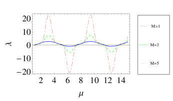
Figure 1: A plot of the eigenvalue $\lambda$ of $B(t_{2},\,t_{1})$ versus $\mu=\frac{t_{2}}{t_{1}}$ for different values of $M$. The dynamics is non-Markovian when $\lambda$ assumes negative values and otherwise it is Markovian.

Another choice $p(t)=e^{-\alpha t}$ corresponds to a CP intermediate map – resulting entirely in a Markovian process. In this case, we also find that $A(t_{2},t_{1})=A(t_{2}-t_{1})$ and this forms a Markov semigroup. However, if $p(t)=e^{-\alpha\,t^{\beta}},\ \ (\beta\neq 1)$, the intermediate map is still CP (and hence Markovian), though $A(t_{2},t_{1})\neq A(t_{2}-t_{1})$ and therefore, it does not constitute a one-parameter semigroup.

Furthermore, we wish to illustrate through this toy model that concurrence of $\rho_{ab}(t)=\frac{1}{d}\,B(t,0)$ (given by $C=\frac{3p(t)-1}{2}$) can never increase as a result of Markovian evolution. This is because ensuing dynamics is a local CP map on the system. Any temporary regain of system-ancilla entanglement during the course of evolution is clearly attributed to the back-flow from environment to the system – which is a signature of non-Markovian process. This feature is displayed in Fig. 2 by plotting the concurrence of $\rho_{ab}(t)$ for different choices of $p(t)$.

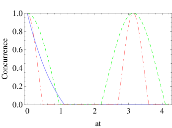
Figure 2: Concurrence $C=\frac{3p(t)-1}{2}$ of the system-ancilla state $\rho_{ab}(t)=\frac{[1-p(t)]}{4}\,I_{2}\otimes I_{2}+p(t)\,|\psi_{\rm ME}\rangle\langle\psi_{\rm ME}|$, vs scaled time $a\,t$, for the following choices (i) Markov process: $p(t)=e^{-at}$ (solid line) and (ii) non-Markov process: $p(t)=\cos^{2M}(a\,t),\ M=1$ (dashed line) and $M=5$ (dot-dashed line). Note that there is a death and re-birth of entanglement (dash, dot-dashed lines) due of back-flow from environment.

V.2 Optical Experiment

Recently, Liu et al Liu reported an optical experiment on the open quantum system constituted by the polarization degree of freedom of photons (system) coupled to the frequency degree of freedom (environment). They reported transition between Markovian and non-Markovian regimes.

The dynamical evolution of the horizontal and vertical poloarization states $|H\rangle,|V\rangle$ of the photon is captured by the following transformation:

$$|H\rangle\langle H\rangle \mapsto |H\rangle\langle H|$$

$$|V\rangle\langle V\rangle \mapsto |V\rangle\langle V|$$

$$|H\rangle\langle V\rangle \mapsto \kappa^{*}(t)\,|H\rangle\langle V|$$ (13)

$$|V\rangle\langle H\rangle \mapsto \kappa(t)\,|V\rangle\langle H|$$

where $\kappa(t)$ denotes the decoherence function, magnitude of which is modelled as (for details see Liu ),

$$|\kappa(t)| = e^{-\frac{1}{2}\sigma^{2}\tau^{2}}\sqrt{1-4A_{1}(1-A_{1})\,\sin^{2}(\tau\,\Delta\omega)}$$

$$\hskip 72.26999pt0\leq A_{1}\leq 1.$$

The corresponding $A$ and $B$ maps (in the $\{HH,HV,VH,VV\}$ basis) are readility identified to be,

$$A(t,0) = \left(\begin{array}[]{cccc}1&0&0&0\\ 0&\kappa^{*}(t)&0&0\\ 0&0&\kappa(t)&0\\ 0&0&0&1\end{array}\right)$$ (19)

$$B(t,0) = \left(\begin{array}[]{cccc}1&0&0&\kappa^{*}(t)\\ 0&0&0&0\\ 0&0&0&0\\ \kappa(t)&0&0&1\end{array}\right)$$ (24)

We construct the intermediate time dynamical map $B(t_{2},t_{1})$ from the corresponding $A(t_{2},t_{1})=A(t_{2},0)A^{-1}(t_{1},0)$ to obtain,

$$B(t_{2},t_{1})=\left(\begin{array}[]{cccc}1&0&0&\frac{\kappa^{*}(t_{2})}{\kappa*(t_{1})}\\ 0&0&0&0\\ 0&0&0&0\\ \frac{\kappa(t_{2})}{\kappa(t_{1})}&0&0&1\end{array}\right).$$ (25)

Eigenvalues of $B(t_{2},t_{1})$ are given by,

$$\lambda_{1,4}=1\pm\left|\frac{\kappa(t_{2})}{\kappa(t_{1})}\right|,\lambda_{2,3}=0.$$ (26)

The eigenvalue $\lambda_{4}$ can assume negative values indicating Markovian/non-Markovian regimes. A plot of the negative eigenvalue as a function of $A_{1}$, for different ratios $t_{2}/t_{1}$, is given in Fig. 3 – where one can clearly see the Markovian ($\lambda_{4}\geq 0$) and non-Markovian ($\lambda_{4}<0$) regimes in this model.

Figure 3: A plot of the eigenvalue $\lambda_{4}$ of $B(t_{2},\,t_{1})$ versus $A_{1}$ for different values of $\mu=\frac{t_{2}}{t_{1}}$.

V.3 Hamiltonian evolution of a two level system coupled to a bath of $N$ spins

We now present a Hamiltonian model, which give rise to explicit structure of time dependence in the open system evolution. Interaction Hamiltonian considered here is Hou

$$H=\frac{A}{\sqrt{N}}\sigma_{z}\sum_{k=1}^{N}\,\sigma_{k\,z}.$$ (27)

This is a simplified model of a hyperfine interaction of a spin-1/2 system with $N$ spin-1/2 nuclear environment in a quantum dot. Taking the initial system-environment state to be $\rho_{S}(0)\otimes\frac{I_{2^{N}}}{2^{N}}$, the dynamical $A$-map is obtained by evaluating ${\rm Tr}_{E}\left[U(t,0)\,\rho_{S}(0)\otimes\frac{I_{2^{N}}}{2^{N}}\,U^{\dagger}(t,0)\right]$ (where $U(t,0)={\rm Exp}[-i\,H\,t]$):

$$A(t,0) = \frac{1}{2}\left(1-x(t)\right)\sigma_{z}\otimes\sigma_{z}+\frac{1}{2}\left(1+x(t)\right)I_{2}\otimes I_{2},$$ (28)

$$x(t)=\cos^{N}\left(\frac{2At}{\sqrt{N}})\right).$$

From this, the intermediate map $A(t_{2},t_{1})$ (see (8)) and in turn the corresponding $B(t_{2},t_{1})$ may be readily evaluated. We obtain,

$$B(t_{2},\,t_{1}) = \frac{1}{2}\,\left(I_{2}\otimes I_{2}+\sigma_{z}\otimes\sigma_{z}\right)$$ (29)

$$+\frac{x(t_{2})}{2x(t_{1})}\left(\sigma_{x}\otimes\sigma_{x}-\sigma_{y}\otimes\sigma_{y}\right).$$

The eigenvalues of $B(t_{2},t_{1})$ are $0,0,1\pm\frac{x(t_{2})}{x(t_{1})}.$ Clearly, the intermediate time dynamics exhibits NCP as one of the eigenvalues i.e., $\lambda=1-\frac{x(t_{2})}{x(t_{1})}$ of $B(t_{2},t_{1})$ can assume negative values. We illustrate regimes of Markovianity/non-Markovianity revealed via positive/negative values of $\lambda$ (plotted as a function of $\mu=t_{2}/t_{1}$) in Fig. 4.

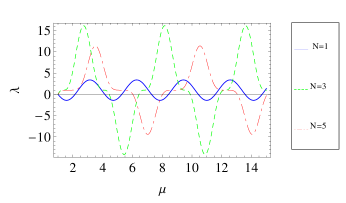
Figure 4: The variation of the eigenvalue $\lambda$ of $B(t_{2},\,t_{1})$ (as a function of $\mu=t_{2}/t_{1}$) from positive to negative values and back with the passage of time for different values of $N$.

V.4 Two qubit unitary evolution

We now consider the open system dynamics arising from the unitary evolution Jordan

$$U(t,0) = e^{-i\,t\,[\omega\,\sigma_{z}\otimes\sigma_{x}]}$$

$$= \cos(\omega\,t/2)\,I_{2}\otimes I_{2}-i\sin(\omega\ t/2)\,\sigma_{z}\otimes\sigma_{x}$$

on the system-environment initial state $\rho_{SE}(0)=\rho_{S}(0)\otimes\rho_{E}(0)=\frac{1}{2}\left(I_{2}+\sigma_{x}\right)\otimes\frac{1}{2}\left(I_{2}+\sigma_{z}\right).$ The $A(t,0)$ map is given by,

$$A(t,0)=\frac{1}{2}\left(1+\cos(\omega\,t)\right)\,I_{2}\otimes I_{2}+\frac{1}{2}\left(1-\cos(\omega\,t)\right)\,\sigma_{z}\otimes\sigma_{z}.$$ (31)

Following (8), we obtain

$$B(t_{2},t_{1}) = \frac{1}{2}\,\left(I_{2}\otimes I_{2}+\sigma_{z}\otimes\sigma_{z}\right)$$ (32)

$$+\frac{\cos(\omega\,t_{2})}{2\cos(\omega t_{1})}\left(\sigma_{x}\otimes\sigma_{x}-\sigma_{y}\otimes\sigma_{y}\right).$$

The eigenvalues of the $B$-map are given by $0,\ 0,1\pm\left|\frac{\cos\omega t_{2}}{\cos\omega t_{1}}\right|$. The eigenvalue $\lambda=1\pm\left|\frac{\cos\omega t_{2}}{\cos\omega t_{1}}\right|$ can assume negative values – bringing out the non-Markovian features prevalent in the dynamical process. Fig. 5 illustrates the transitions from Markovianity to non-Markovianity.

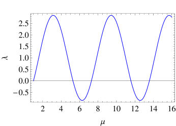
Figure 5: The plot of the eigenvalue $\lambda=1-\left|\frac{\cos\omega t_{2}}{\cos\omega t_{1}}\right|$ as a function of $\mu=\frac{t_{2}}{t_{1}}$. The periodic transitions of $\lambda$ from positive to negative values indicates the transition of the process from Markovian to non-Markovian.

This model, with initially correlated states, has been explored before in Refs. Jordan ; AKRUS and the dynamical map turned out to be NCP throughout not merely in the intermediate time interval).

VI Summary

In conclusion, a few remarks on a variety of definitions of non-Markovianity in the recent literature may be recalled here. Mainly the focus has been towards capturing the violation of semi-group property AKRUR ; AKRUS or more recently – its two-parameter generalization viz the divisibility of the dynamical map div ; RHP . Yet another measure, where non-Markovianity BLP is attributed to increase of distinguishability of any pairs of states (as a result of the partial back-flow of information from the environment into the system) and is quantified in terms of trace distance of the states. It has been shown that the two different measures of non-Markovianity – one based on the divisibility of the dynamical map RHP and the other based upon the distinguishability of quantum states BLP – need not agree with each other haikka . A modified version of the criterion of Ref. RHP was proposed recently Hou . In this paper we have established the interplay of stochastic $A$ and dynamical $B$ maps at intermediate times, revealing Markovian/non-Markovian regimes. We have explored four different examples revealing the features of intermediate time maps originating from variety of physical mechanisms : (i) A toy model map inspired by general considerations based on Jamiolkowski isomorphism – which explores a two qubit Werner state with time-dependent noise parameter as a dynamical map (ii) A reinterpretation of the phenomenological model explaining the recent optical experiment by Liu et. al., Liu in terms of NCP nature of the intermediate $B$ map. (iii) Hamiltonian evolution describing the hyperfine interaction of a spin-1/2 system with $N$ spin-1/2 nuclear environment in a quantum dot Hou displaying Markovian/non-Markovian behaviour and (iv) Unitary evolution of Jordan et. al.,  Jordan – wherein initial system-environment two qubit is chosen in a product state. Here too, intermediate time dynamical map exhibits Markov/non-Markov regimes. It is interesting to note that the dynamics had been identified to be NCP throughout not merely in the intermediate time interval – when initially correlated states were employed Jordan ; AKRUS . Placing these two results together, brings forth that the source of non-Markovianity in this model is attributable entirely to the unitary dynamics — rather than initial correlations of system-environment qubits. We have thus exposed the underlying features of intermediate time $A$ and $B$ maps to bring out clearly if the dynamics relies on past history of the states or not.

References

- (1) H.-P. Breuer and F. Petruccione, The Theory of Open Quantum Systems (Oxford Univ. Press, Oxford, 2007).
- (2) R. Alicki and K. Lendi, Quantum Dynamical Semigroups and Applications (Springer, Berlin, 1987).
- (3) M. A. Nielsen and I. L. Chuang, Quantum Computation and Quantum Information (Cambridge Univ. Press, Cambridge, 2000).
- (4) M. D. Choi, Can. J. Math. 24, 520 (1972); Linear Algebra and Appl. 10, 285 (1975).
- (5) A. Jamiolkowski, Reports on Mathematical Physics, 3, (1972).
- (6) E. C. G. Sudarshan, P. Mathews, and J. Rau, Phys. Rev. 121, 920 (1961); T. F. Jordan and E. C. G. Sudarshan, J. Math. Phys. 2, 772 (1961).
- (7) G. Lindblad, Comm. Math. Phy. 48, 119 (1976).
- (8) V. Gorini, A. Kossakowski, and E. C. G. Sudarshan, J. Math. Phys. 17, 821 (1976).
- (9) M. M. Wolf, J. Eisert, T. S. Cubitt and J. I. Cirac, Phys. Rev. Lett. 101, 150402 (2008).
- (10) A. Rivas, S. F. Huelga and M. B. Plenio, Phys. Rev. Lett. 105, 050403 (2010).
- (11) T. F. Jordan, A. Shaji, and E. C. G. Sudarshan, Phys. Rev. A70, 052110 (2004).
- (12) C. A. Rodŕguez-Rosario and E. C. G. Sudarshan, e-print arXiv:0803.1183 [quant-ph].
- (13) C. A. Rodríguez-Rosario, K. Modi, A. Kuah, A. Shaji, and E. C. G. Sudarshan, J. Phys. A 41, 205301 (2008).
- (14) K. Modi and E. C. G. Sudarshan, Phys. Rev. A81, 052119 (2010).
- (15) A. R. Usha Devi, A. K. Rajagopal, Sudha, Phys. Rev. A83, 022109 (2011).
- (16) H.-P. Breuer, Phys. Rev. A69 022115 (2004); ibid. 70, 012106 (2004); S. Daffer, K. Wódkiewicz, J. D. Cresser, and J. K. McIver, Phys. Rev. A70, 010304 (2004); H.-P. Breuer and B. Vacchini,Phys. Rev. Lett. 101 (2008) 140402; Phys. Rev. E79, 041147 (2009); A. Kossakowski and R. Rebolledo, Open Syst. Inf. Dyn. 14, 265 (2007); 15, 135 (2008); 16, 259 (2009); D. Chruściński and A. Kossakowski, Phys. Rev. Lett. 104, 070406 (2010)
- (17) A. K. Rajagopal, A. R. Usha Devi and R. W. Rendell, Phys. Rev. A82, 042107 (2010).
- (18) H.-P. Breuer, E.-M. Laine, J. Piilo, Phys. Rev.Lett. 103, 210401 (2009); E.-M. Laine, J. Piilo, H.-P. Breuer, Phys. Rev. A81, 062115 (2010).
- (19) P. Haikka, J.D. Cresser and S. Maniscalco Phys. Rev. A83, 012112 (2011).
- (20) D. Chruściński, A. Kossakowski and A. Rivas, Phys. Rev. A83, 052128 (2011)
- (21) S. C. Hou, X. X. Yi, S. X. Yu and C. H. Oh, Phys. Rev. A83, 062115 (2011).
- (22) The dynamical evolution of the system density matrix is not a local unitary operation, when ’memoryless reservoir approximation’ holds – but it is governed by an irreversible, stochastic map.
- (23) K. G. H. Vollbrecht and R. F. Werner, Phys. Rev. A64, 062307 (2001).
- (24) B.L. Liu, L. Li, Y.-F. Huang, C.-F. Li, G.-C. Guo, E.-M Laine, H.-P. Breuer and J. Piilo, Nature Physics, 7, 931 (2011).