Effect of mesoscopic fluctuations on equation of state in cluster-forming systems

Abstract

Equation of state for systems with particles self-assembling into aggregates is derived within a mesoscopic theory combining density functional and field-theoretic approaches. We focus on the effect of mesoscopic fluctuations in the disordered phase. The pressure – volume fraction isotherms are calculated explicitly for two forms of the short-range attraction long-range repulsion potential. Mesoscopic fluctuations lead to an increased pressure in each case, except for very small volume fractions. When large clusters are formed, the mechanical instability of the system is present at much higher temperature than found in mean-field approximation. In this case phase separation competes with the formation of periodic phases (colloidal crystals). In the case of small clusters, no mechanical instability associated with separation into dilute and dense phases appears.

Key words: clusters, self-assembly, equation of state, mesoscopic fluctuations

PACS: 61.20.Gy, 64.10.+h, 64.60.De, 64.75.Yz

Abstract

Рiвняння стану для систем частинок, що самоскупчуються в агрегати, є отримане в рамках мезоскопiчної теорiї, що поєднує метод функцiоналу густини i теоретико-польовий пiдхiд. Ми дослiджуємо вплив мезоскопiчних флуктуацiй у невпорядкованiй фазi. Явно обчислено iзотерми ‘тиск – об’ємна частка’ для двох наборiв параметрiв потенцiалу короткосяжне притягання плюс далекосяжне вiдштовхування. В кожному випадку врахування мезоскопiчних флуктуацiй приводить до пiдвищення тиску, за винятком дуже малих об’ємних часток. Коли утворюються великi кластери, механiчна нестiйкiсть системи присутня при набагато вищих температурах, нiж це було отримано в наближеннi середнього поля. В цьому випадку фазове вiдокремлення конкурує iз формуванням перiодичних фаз (колоїдних кристалiв). У випадку малих кластерiв механiчна нестiйкiсть, пов’язана з вiдокремленням в розрiджену i густу фази, не виникає.

Ключовi слова: кластери, самоскупчення, рiвняння стану, мезоскопiчнi флуктуацiї

1 Introduction

Recent experimental [1, 3, 2, 4], theoretical [7, 9, 10, 5, 11, 6, 8] and simulation [14, 15, 8, 12, 16, 13] studies reveal that in many systems with competing interactions, clusters or aggregates of different sizes and shapes are formed. These objects in certain thermodynamic states can form ordered structures in space [5, 11, 12]. Notable examples include charged globular proteins in water [1, 17, 3, 13], and mixtures of small nonadsorbing polymers with charged colloids or micelles [1, 2, 18]. Interactions (or in fact effective interactions) in the latter systems can be described by the model potential consisting of short-range attraction, resulting from solvophobic or depletion interactions, and long-range repulsion, resulting from screened electrostatic potential (SALR potential).

Systems containing clusters or aggregates are inhomogeneous on the length scale associated with the average size of the aggregates and average distance between them. The corresponding length scale of the inhomogeneities is significantly larger than the size of the particles. Fluctuations on the mesoscopic length scale corresponding to displacements of the aggregates have an important impact on the grand potential, and thus on the equation of state (EOS). Derivation of an accurate EOS for inhomogeneous systems is less trivial than in the case of homogeneous systems, since it is necessary to perform summation over different spatial distributions of the clusters and over all deformations of them.

Contribution to the grand potential associated with mesoscopic fluctuations can be calculated in the field-theoretic approach [5, 11]. In principle, this contribution can be obtained in the perturbation expansion in terms of Feynman diagrams. In practice, an approximate result can be analytically obtained in the self-consistent Hartree approximation [19, 5, 6]. A formal expression for the fluctuation contribution to the grand potential has been derived in references [19, 5, 6]. However, its explicit form with the chemical potential expressed in terms of temperature and density has not been determined yet. The EOS isotherms for various forms of the SALR potential were not analyzed, and the effect of the mesoscopic fluctuations on pressure remains an open question.

It is important to note that various forms of the SALR potential are associated with different properties of the systems. Depending on the ratios between the strengths and ranges of the attractive and repulsive parts of the potential, separation into uniform phases, formation of clusters of various sizes and shapes (globules, cylinders, slabs) in the so-called microsegregation, or isolated individual particles may occur. In certain conditions, the clusters can be periodically distributed in space in the periodic phases whose densities are smaller than the density of the liquid phase [12, 5, 11]. Possible types of the phase diagram for different SALR potentials are shown in figure 1 (see also references [9, 10, 5]).

Figure 1: Types of possible phase diagrams for the SALR potentials, shown schematically. From the left to the right panel the role of the repulsion increases. ‘p’ indicates the stability region of the periodic phases of different symmetries. The disordered fluid close to the stability region of the periodic phases is inhomogeneous, i.e. clusters are formed, but their positions are correlated only at short distances. In this work we are interested in systems exhibiting the phase behaviour shown in the right (System 1) and the central (System 2) panel.

Properties of the disordered phase can be influenced by the periodic phases for thermodynamic states close to the stability of the latter. We expect that the disordered phase, although the long-range order is absent, is inhomogeneous on the mesoscopic length scale and resembles ‘molten periodic phases’. In this respect the inhomogeneous disordered phase is similar to microemulsion which can be interpreted as molten lyotropic liquid crystal.

In this work we focus on the stable or metastable disordered inhomogeneous phase in which clusters are formed, but they do not form any ordered structure. We derive the EOS with the contribution from mesoscopic length-scale fluctuations included. We calculate the explicit form of the EOS for two representative examples of the SALR potential within the self-consistent Hartree approximation. The first system corresponds to the formation of small clusters, and the gas-liquid separation is unstable for all temperatures in the mean-field (MF) approximation (figure 1, right panel). In the second system, large clusters are formed. The gas-liquid separation is present in this system as a stable or a metastable transition for low temperatures (figure 1, central panel). We shall compare the effect of mesoscopic fluctuations in these two cases on the isotherms $P(\zeta)$, where $\zeta$ is the volume fraction of particles and $P$ is pressure.

In the next section we briefly summarize the mesoscopic approach. In section 3 the EOS is obtained by two methods. In section 3.1 we consider mesoscopic fluctuations about the average volume fraction, while in section 3.2 fluctuations about the most probable volume fraction are included. The formulas derived in section 3 are evaluated for the two versions of the SALR potential in section 4. We obtain a completely different effect of the mesoscopic fluctuations in these two cases. The two approaches (sections 3.1 and 3.2) yield very close results provided that the relative fluctuation contribution to the average volume fraction is small. For larger fluctuation-induced shifts of the volume fraction, only qualitative agreement of the two methods is obtained. Short summary is presented in section 5.

2 Short summary of the mesoscopic description

We consider a local volume fraction of particles, i.e. the microscopic volume fraction averaged over mesoscopic regions, as an order parameter [6]. The corresponding mesoscopic volume fraction varies on a length scale larger than the size of the particles, and the characteristic size of inhomogeneities is the upper limit for the mesoscopic length scale. A particular form of the mesoscopic volume fraction can be considered as a constraint on the microscopic states. The corresponding mesostate is a subset of microstates compatible with the imposed constraint. The mesoscopic volume fraction (or the mesostate) was defined in references [5, 6]. For a one-component case we fix the mesoscopic length scale $R\geqslant\sigma/2$ and consider spheres $S_{R}({\mathbf{r}})$ of radius $R$ and centers at $\mathbf{r}$ that cover the whole volume $V$ of the system. We define the mesoscopic volume fraction at $\mathbf{r}$ by

$$\zeta(\mathbf{r}):=\frac{1}{V_{S}}\int_{\mathbf{r^{\prime}}\in S_{R}(\mathbf{r})}\hat{\zeta}(\mathbf{r^{\prime}},{\cal M}),$$ (2.1)

where $V_{S}=4\pi R^{3}/3$, and the microscopic volume fraction in the microstate ${\cal M}=\{\{{\bf r}_{i}\}_{i=1,\ldots,N}\}$ is defined by

$$\hat{\zeta}({\bf r},{\cal M}):=\sum_{i=1}^{N}\theta\left(\frac{\sigma}{2}-|{\bf r}-{\bf r}_{i}|\right),$$ (2.2)

where $\theta(r)$ is the Heaviside unit step function. The microscopic volume fraction is equal to $1$ at points that are inside one of the hard spheres, and zero otherwise. Integrated over the system volume, it yields the volume occupied by the particles. The mesoscopic volume fraction at ${\bf r}$ is equal to the fraction of the volume of the sphere $S_{R}({\bf r})$ that is occupied by the particles. Note that $\zeta({\bf r})$ takes the same value if one particle is entirely included in this sphere, independently of the precise position of its centre. Thus, $\zeta({\bf r})$ gives less precise information on the distribution of particles than $\hat{\zeta}({\bf r})$. In the disordered phase $\zeta({\bf r})$ is independent of ${\bf r}$ and equals the fraction of the total volume that is occupied by the particles. The mesostate can be imagined as a fixed distribution of centers of clusters, with arbitrary distribution of particles within the clusters, and small modifications of their shapes. Probability of the mesostate $\zeta$ is given by [5, 6]

$$p[\zeta]=\frac{\mathrm{e}^{-\beta\Omega_{\mathrm{co}}[\zeta]}}{\Xi}\,,$$ (2.3)

where

$$\Xi=\int\nolimits^{\prime}D\zeta\,\mathrm{e}^{-\beta\Omega_{\mathrm{co}}[\zeta]}.$$ (2.4)

The functional integral $\int^{{}^{\prime}}D\zeta$ in (2.4) is over all mesostates,

$$\Omega_{\mathrm{co}}=U[\zeta]-TS[\zeta]-\mu N[\zeta],$$ (2.5)

where $U,S,N$ are the internal energy, entropy and the number of molecules respectively in the system with the constraint of compatibility with the mesostate $[\zeta]$ imposed on the microscopic volume fractions. $U$ is given by the well known expression

$$U[\zeta]=\frac{1}{2}\int_{\bf r_{1}}\int_{\bf r_{2}}V_{\mathrm{co}}({\bf r}_{1}-{\bf r}_{2})\zeta({\bf r}_{1})\zeta({\bf r}_{2}),$$ (2.6)

where for spherically symmetric interactions

$$V_{\mathrm{co}}({\bf r}_{1}-{\bf r}_{2})=V(r_{12})g_{\mathrm{co}}({\bf r}_{1}-{\bf r}_{2}),$$ (2.7)

$r_{12}=|{\bf r}_{1}-{\bf r}_{2}|$, $v^{2}V(r_{12})$ is the interaction potential, $v=\pi\sigma^{3}/6$ is the volume of the particle, and $g_{\mathrm{co}}({\bf r}_{1}-{\bf r}_{2})$ is the microscopic pair correlation function for the microscopic volume fraction in the system with the constraint of compatibility with the mesostate imposed on the microscopic states. The grand potential can be written in the form

$$\beta\Omega[\bar{\zeta}]=\beta\Omega_{\mathrm{co}}[\bar{\zeta}]-\log\Xi_{\mathrm{fluc}}\,,$$ (2.8)

where

$$\Xi_{\mathrm{fluc}}=\int D\phi\,\mathrm{e}^{-\beta H_{\mathrm{fluc}}[\bar{\zeta},\phi]},$$ (2.9)

$$H_{\mathrm{fluc}}[\bar{\zeta},\phi]=\Omega_{\mathrm{co}}[\bar{\zeta}+\phi]-\Omega_{\mathrm{co}}[\bar{\zeta}]=\sum_{n=1}\int_{\bf r_{1}}\ldots\int_{\bf r_{n}}\frac{C^{\mathrm{co}}_{n}[\bar{\zeta}]}{n!}\phi({\bf r}_{1})\ldots\phi({\bf r}_{n}).$$ (2.10)

The average mesoscopic volume fraction, $\bar{\zeta}$, corresponds to the minimum of $\Omega$, and must satisfy the equation

$$\frac{\delta\beta\Omega_{\mathrm{co}}[\bar{\zeta}]}{\delta\bar{\zeta}({\bf r})}+\left\langle\frac{\delta(\beta H_{\mathrm{fluc}})}{\delta\bar{\zeta}({\bf r})}\right\rangle=0,$$ (2.11)

where the averaging is over the fields $\phi$ with the probability $\propto\exp(-\beta H_{\mathrm{fluc}}[\bar{\zeta},\phi])$. Note that when $C^{\mathrm{co}}_{n}[\bar{\zeta}]=0$ for odd $n$, then the second term on the LHS in (2.11) vanishes, and the average volume fraction coincides with the most probable volume fraction $\zeta_{0}$ given by

$$\left.\frac{\delta\beta\Omega_{\mathrm{co}}[\zeta]}{\delta\zeta({\bf r})}\right|_{\zeta=\zeta_{0}}=0.$$ (2.12)

By contrast, when $C^{\mathrm{co}}_{n}[\bar{\zeta}]\neq 0$ for odd $n$, then $\bar{\zeta}\neq\zeta_{0}$.

In order to evaluate the fluctuation contribution to $\Omega[\bar{\zeta}]$ we decompose $H_{\mathrm{fluc}}[\bar{\zeta},\phi]$ into two parts

$$H_{\mathrm{fluc}}[\bar{\zeta},\phi]={\cal H}_{\mathrm{G}}[\bar{\zeta},\phi]+\Delta{\cal H}[\bar{\zeta},\phi],$$ (2.13)

where in the disordered phase

$${\cal H}_{\mathrm{G}}[\bar{\zeta},\phi]=\frac{1}{2}\int_{\bf k}\tilde{\phi}({\bf k})\tilde{C}_{2}({\bf k},\bar{\zeta})\tilde{\phi}(-{\bf k}),$$ (2.14)

and $\tilde{C}_{2}({\bf k},\zeta)$ is the Fourier transform of

$$C_{2}(r_{12},\zeta)=\frac{\delta^{2}\beta\Omega[\zeta]}{\delta\zeta({\bf r}_{1})\delta\zeta({\bf r}_{2})}\,.$$ (2.15)

The above function calculated for $\zeta=\bar{\zeta}$ is related to the direct correlation function [20].

Assuming $\Delta{\cal H}\ll{\cal H}_{\mathrm{G}}$, we obtain [19, 5]

$$\beta\Omega[\bar{\zeta}]\approx\beta\Omega_{\mathrm{co}}[\bar{\zeta}]-\log\int D\phi\,\mathrm{e}^{-\beta{\cal H}_{\mathrm{G}}}+\langle\beta\Delta{\cal H}\rangle_{\mathrm{G}}+O\left(\langle\beta\Delta{\cal H}\rangle_{\mathrm{G}}^{2}\right),$$ (2.16)

where $\langle\ldots\rangle_{\mathrm{G}}$ denotes the averaging with the Gaussian Boltzmann factor $\propto\mathrm{e}^{-\beta{\cal H}_{\mathrm{G}}}$.

Since $P=-\Omega/V$, approximate EOS can be obtained from (2.16) calculated for $\bar{\zeta}$ satisfying (2.11), when $\Omega_{\mathrm{co}}[\bar{\zeta}]$ (see (2.5)) is known. The chemical potential in (2.16) should be expressed in terms of $T$ and $\bar{\zeta}$; its form as a function of $T$ and $\bar{\zeta}$ can be determined from equation (2.11). In order to evaluate the second term in equation (2.11), we need approximate forms of the correlation functions. In the lowest order approximation, it is necessary to determine

$$\langle\tilde{\phi}({\bf k})\tilde{\phi}(-{\bf k})\rangle=\tilde{G}_{2}(k,\bar{\zeta})=1/\tilde{C}_{2}(k,\bar{\zeta}).$$ (2.17)

3 Approximate results for the fluctuation contributions to the EOS, density and chemical potential

In this section we derive an explicit form of the EOS $P(\bar{\zeta},T)$, the density shift, $\Delta\zeta=\bar{\zeta}-\zeta_{0}$, and the chemical potential $\mu(\bar{\zeta},T)$ under the following assumptions: (i) local density approximation for $S[\zeta]$ and (ii) the lowest-order approximation for the second term in (2.11). In the local density approximation we have

$$-TS[\zeta]=\int_{\bf r}f_{\mathrm{h}}(\zeta({\bf r})),$$ (3.1)

where $f_{\mathrm{h}}(\zeta)$ is the free-energy density of the hard-sphere system with dimensionless density $\rho^{*}=6\zeta/\pi$. We assume the Percus-Yevick approximation

$$\beta f_{\mathrm{h}}(\zeta)=\rho^{*}\ln(\rho^{*})-\rho^{*}+\rho^{*}\Bigg{[}\frac{3\zeta(2-\zeta)}{2(1-\zeta)^{2}}-\ln(1-\zeta)\Bigg{]}.$$ (3.2)

In the local density approximation $C_{n}^{\mathrm{co}}[\zeta]$ are just functions of $\zeta$ in the disordered phase, and we can simplify the notation, introducing

$$A_{n}(\zeta)=\frac{\mathrm{d}^{n}[\beta f_{\mathrm{h}}(\zeta)]}{\mathrm{d}\zeta^{n}}\,.$$ (3.3)

For $n>2$ we have

$$C_{n}^{\mathrm{co}}[\zeta]=A_{n}(\zeta),$$ (3.4)

whereas for $n=2$

$$\tilde{C}^{\mathrm{co}}_{2}(k,\zeta)=\beta\tilde{V}_{\mathrm{co}}(k)+A_{2}(\zeta),$$ (3.5)

where in the disordered phase $\tilde{C}_{2}^{\mathrm{co}}(k,\zeta)$ is the Fourier transform of the function

$$C^{\mathrm{co}}_{2}(r_{12},\zeta)=\frac{\delta^{2}\beta\Omega_{\mathrm{co}}[\zeta]}{\delta\zeta({\bf r}_{1})\delta\zeta({\bf r}_{2})}\,.$$ (3.6)

Equations (3.2) and (2.6) define the functional $\Omega_{\mathrm{co}}$ for a given form of $V_{\mathrm{co}}$ (equation (2.7)).

From equation (2.3) it follows that the most probable fluctuations correspond to the wavenumbers $k=k_{\mathrm{b}}$ for which $\tilde{V}_{\mathrm{co}}(k)$ assumes the minimum, and the inhomogeneities on the length scale $2\pi/k_{\mathrm{b}}$ are energetically favored when $\tilde{V}_{\mathrm{co}}(k_{\mathrm{b}})<0$. In this work we focus on the effect of the self-assembly into aggregates. Therefore, we restrict our attention to $\tilde{V}_{\mathrm{co}}(k)$ which assumes the minimum for $k_{\mathrm{b}}>0$, and $\tilde{V}_{\mathrm{co}}(k_{\mathrm{b}})<0$ [5, 11]. Since the fluctuations with the wavenumber $k\approx k_{\mathrm{b}}$ are most probable, they yield the main fluctuation contribution to the grand potential (2.16). For such fluctuations we can make the approximation

$$\beta\tilde{V}_{\mathrm{co}}(k)\approx\beta\tilde{V}_{\mathrm{co}}(k_{\mathrm{b}})+\beta\tilde{V}_{\mathrm{co}}^{(2)}(k_{\mathrm{b}})(k-k_{\mathrm{b}})^{2}/2+\ldots$$ (3.7)

As the energy scale we choose the excess energy associated with the fluctuations having unit amplitude and the wavenumber $k_{\mathrm{b}}$, and introduce the notation

$$\beta^{*}=1/T^{*}=\beta|\tilde{V}_{\mathrm{co}}(k_{\mathrm{b}})|,$$ (3.8)

$$v_{2}^{*}=\frac{\tilde{V}_{\mathrm{co}}^{(2)}(k_{\mathrm{b}})}{2|\tilde{V}_{\mathrm{co}}(k_{\mathrm{b}})|}$$ (3.9)

and

$$v_{0}^{*}=\frac{\tilde{V}_{\mathrm{co}}(0)}{\tilde{V}_{\mathrm{co}}(k_{\mathrm{b}})}\,.$$ (3.10)

3.1 Fluctuations around the average volume fraction

In this subsection we consider fluctuations about the average value $\bar{\zeta}$. We shall first determine the chemical potential as a function of $\bar{\zeta}$ and $T^{*}$ from (2.11). In order to calculate the second term in (2.11), we assume that relevant fluctuations are of small amplitudes, and truncate the expansion in (2.10) at the fourth-order term. Next we insert the derivative with respect to $\bar{\zeta}$ of the RHS of equation (2.10) truncated at the quadratic term in $\phi$, and we obtain from (2.11) and (2.5) an approximate equation for the rescaled chemical potential, $\bar{\mu}=6\mu/(\pi\sigma^{3})$, of the form

$$\beta\bar{\mu}\approx\beta\bar{\mu}^{\mathrm{MF}}(\bar{\zeta})+\frac{A_{3}(\bar{\zeta})}{2}{\cal G}(\bar{\zeta}),$$ (3.11)

where

$$\beta\bar{\mu}^{\mathrm{MF}}(\bar{\zeta})=\beta\tilde{V}_{\mathrm{co}}(0)\bar{\zeta}+\beta f_{\mathrm{h}}^{\prime}(\bar{\zeta})$$ (3.12)

and the last term in (3.11) is the fluctuation contribution with

$${\cal G}(\zeta)=\int_{\bf k}\tilde{G}_{2}(k,\zeta)=G_{2}(0,\zeta).$$ (3.13)

The same expression can be obtained from $\langle\phi\rangle=0$, when (2.13), (2.14) and the approximation

$$\mathrm{e}^{-\beta H_{\mathrm{fluc}}}=\mathrm{e}^{-\beta H_{\mathrm{G}}}\Big{[}1-\beta\Delta H+O\left(\Delta H^{2}\right)\Big{]}$$ (3.14)

are used. The approximation (3.11) is valid as long as the correction term is not larger than the MF result. When considering particular cases we shall verify if this is the case. The fluctuation contribution to the direct correlation function (2.15) is obtained by calculating the second derivative of the second term on the RHS of (2.8) with respect to $\bar{\zeta}$. In the consistent approximation we insert in the obtained expression the appropriate derivatives of $H_{\mathrm{fluc}}$ (equation (2.10)) with the expansion in $\phi$ truncated at the second order. The result is given by [19, 21, 5, 6]

$$\tilde{C}_{2}(k,\zeta)\approx\tilde{C}^{\mathrm{co}}_{2}(k,\zeta)+\frac{A_{4}(\zeta)}{2}{\cal G}(\zeta).$$ (3.15)

Equations (3.15), (2.17) and (3.13) should be solved self-consistently.

The fluctuation induced shift of the volume fraction, $\Delta\zeta=\bar{\zeta}-\zeta_{0}$, can be obtained from (2.11) by expanding the first term on the LHS about $\zeta_{0}$,

$$\tilde{C}_{2}^{\mathrm{co}}(0,\zeta_{0})\Delta\zeta+\sum_{n=2}^{\infty}\frac{C_{n+1}^{\mathrm{co}}[\zeta_{0}]}{n!}\Delta\zeta^{n}=-\left\langle\frac{\delta(\beta H_{\mathrm{fluc}})}{\delta\bar{\zeta}({\bf r})}\right\rangle.$$ (3.16)

For small $\Delta\zeta$ we can truncate the expansion in (3.16) at the first term. When the RHS in (3.16) is approximated as in the calculation of $\bar{\mu}$ from (2.11), we obtain the result

$$\Delta\zeta\approx-\frac{A_{3}(\zeta_{0})}{2\tilde{C}_{2}(0,\zeta_{0})}{\cal G}(\bar{\zeta})\approx-\frac{A_{3}(\zeta_{0})}{2\tilde{C}_{2}(0,\zeta_{0})+A_{3}(\zeta_{0}){\cal G}^{\prime}(\zeta_{0})}{\cal G}(\zeta_{0}).$$ (3.17)

We used the approximations: $A_{3}(\bar{\zeta})=A_{3}(\zeta_{0})+A_{4}(\zeta_{0})\Delta\zeta+O\left(\Delta\zeta^{2}\right)$, ${\cal G}(\bar{\zeta})={\cal G}(\zeta_{0})+{\cal G}^{\prime}(\zeta)\Delta\zeta+O\left(\Delta\zeta^{2}\right)$ and equation (3.15).

For the potential given in (3.7) the approximate form of ${\cal G}$ is [22, 19, 21, 5]

$${\cal G}(\zeta)=\frac{2a\sqrt{T^{*}}}{Z(\zeta)}\,,$$ (3.18)

where

$$a=\frac{k_{\mathrm{b}}^{2}}{4\pi\sqrt{v_{2}^{*}}}$$ (3.19)

and $Z(\zeta)=\sqrt{\tilde{C}_{2}(k_{\mathrm{b}},\zeta)}$. The above approximation is valid for $\tilde{C}_{2}(k_{\mathrm{b}},\zeta)\ll\beta^{*}v_{2}^{*}k_{\mathrm{b}}^{2}$ [22, 19, 21, 5]. The equation (3.15) for $k=k_{\mathrm{b}}$ takes the form

$$Z(\zeta)^{3}=Z(\zeta)\tilde{C}_{2}^{\mathrm{co}}(k_{\mathrm{b}},\zeta)+A_{4}(\zeta)a\sqrt{T^{*}},$$ (3.20)

and the explicit expression for $Z$ is

$$Z(\zeta)=\frac{W(\zeta)}{6}+\frac{2\tilde{C}_{2}^{\mathrm{co}}(k_{\mathrm{b}},\zeta)}{W(\zeta)}$$ (3.21)

with

$$W(\zeta)=\left\{108A_{4}(\zeta)a\sqrt{T^{*}}+12\sqrt{-12\tilde{C}_{2}^{\mathrm{co}}(k_{\mathrm{b}},\zeta)^{3}+81\left[A_{4}(\zeta)a\sqrt{T^{*}}\right]^{2}}\right\}^{1/3}.$$ (3.22)

The fluctuation contribution in equation (2.16) for the approximations (3.15)–(3.20) was calculated in references [22, 19, 21, 5], and has the form

$$\beta\Omega[\bar{\zeta}]\approx\beta\Omega_{\mathrm{co}}[\bar{\zeta}]+2a\sqrt{T^{*}}Z(\bar{\zeta})V-\frac{A_{4}(\bar{\zeta}){\cal G}(\bar{\zeta})^{2}}{8}V.$$ (3.23)

Taking into account (3.11) and (3.2), we obtain from (3.23) the explicit form of the EOS

$$\beta P(\bar{\zeta})=\beta P^{\mathrm{MF}}(\bar{\zeta})+F(\bar{\zeta},T^{*}),$$ (3.24)

where

$$\beta P^{\mathrm{MF}}(\bar{\zeta})=-\frac{\beta^{*}v_{0}^{*}}{2}\bar{\zeta}^{2}+\bar{\zeta}\frac{\mathrm{d}\beta f_{\mathrm{h}}(\bar{\zeta})}{\mathrm{d}\bar{\zeta}}-\beta f_{\mathrm{h}}(\bar{\zeta})=-\frac{\beta^{*}v_{0}^{*}}{2}\bar{\zeta}^{2}+\rho^{*}\frac{\bar{\zeta}^{2}+\bar{\zeta}+1}{\left(1-\bar{\zeta}\right)^{3}}$$ (3.25)

and

$$F(\bar{\zeta},T^{*}) = \frac{a\sqrt{T^{*}}A_{3}(\bar{\zeta})\bar{\zeta}}{Z(\bar{\zeta})}-2a\sqrt{T^{*}}Z(\bar{\zeta})+\frac{a^{2}A_{4}(\bar{\zeta})T^{*}}{2Z(\bar{\zeta})^{2}}$$ (3.26)

$$= \frac{a\sqrt{T^{*}}}{2}\left[\frac{2A_{3}(\bar{\zeta})\bar{\zeta}-\tilde{C}_{2}^{\mathrm{co}}(k_{\mathrm{b}},\bar{\zeta})}{Z(\bar{\zeta})}-3Z(\bar{\zeta})\right].$$

The second equality in (3.25) is valid for the PY approximation for $f_{\mathrm{h}}$. In order to obtain the last equality in (3.26), equation (3.20) was used.

3.2 Fluctuations around the most probable volume fraction

In the previous subsection we considered fluctuations about the average value, which in general differs from the most probable value of the volume fraction. In principle, it is possible to consider equations analogous to (2.8) and (2.10), but with $\bar{\zeta}$ replaced by $\zeta_{0}$. In this new approach equation (2.12) is satisfied, and thus the expansion in (2.10) starts with $n=2$ ($C_{1}^{\mathrm{co}}[\zeta_{0}]=0$). On the other hand, $\langle\phi\rangle=\bar{\zeta}-\zeta_{0}\neq 0$. The results obtained in the two approaches — with included fluctuations around the average value or around the most probable value — should be the same in the exact theory. However, when the fluctuation contribution is obtained in an approximate theory, the results may depend on the validity of the assumptions made in the two approaches. In this section we derive an alternative version of the EOS, based on the contribution from the fluctuations around the most probable value. From (2.12) we obtain for the chemical potential

$$\bar{\mu}(\zeta_{0})=\bar{\mu}^{\mathrm{MF}}(\zeta_{0})$$ (3.27)

with $\bar{\mu}^{\mathrm{MF}}$ given in equation (3.12). We consider (2.13) with $\bar{\zeta}$ replaced by $\zeta_{0}$, and the approximation (3.14). In the above, $H_{\mathrm{G}}$ is given in equation (2.14) with $\tilde{C}_{2}(k,\zeta_{0})=1/\tilde{G}_{2}(k,\zeta_{0})$, where $\tilde{G}_{2}(k,\zeta_{0})=\langle\tilde{\phi}({\bf k})\tilde{\phi}(-{\bf k})\rangle$, and

$$\Delta H = \frac{1}{2}\int_{\bf r^{\prime}}\int_{\bf r^{\prime\prime}}\phi({\bf r}^{\prime})\left[C_{2}^{\mathrm{co}}\left({\bf r}^{\prime}-{\bf r}^{\prime\prime},\zeta_{0}\right)-C_{2}\left({\bf r}^{\prime}-{\bf r}^{\prime\prime},\zeta_{0}\right)\right]\phi({\bf r}^{\prime\prime})+\int_{\bf r}\frac{A_{3}(\zeta_{0})}{3!}\phi({\bf r})^{3}+\int_{\bf r}\frac{A_{4}(\zeta_{0})}{4!}\phi({\bf r})^{4}+\ldots$$

Note that the function $\tilde{G}_{2}(k,\zeta_{0})$ defined here differs from the correlation function, because in this case $\langle\phi({\bf r})\rangle\neq 0$. Taking into account that for $H_{\mathrm{G}}$ of the form (2.13) there holds $\int D\phi\mathrm{e}^{-\beta H_{\mathrm{G}}}\phi^{2n+1}=0$, we obtain the expression

$$\langle\phi({\bf r})\rangle\approx\frac{-\int D\phi\,\frac{1}{3!}\int_{\bf r^{\prime}}\int_{\bf r^{\prime\prime}}\int_{\bf r^{\prime\prime\prime}}A_{3}(\zeta_{0})\phi\left({\bf r}^{\prime}\right)\phi\left({\bf r}^{\prime\prime}\right)\phi\left({\bf r}^{\prime\prime\prime}\right)\phi({\bf r})\mathrm{e}^{-\beta H_{\mathrm{G}}}}{\Xi_{\mathrm{fluc}}}\,.$$ (3.29)

Finally, the lowest-order result is

$$\bar{\zeta}=\zeta_{0}+\langle\phi\rangle\approx\zeta_{0}-\frac{A_{3}(\zeta_{0})}{2\tilde{C}_{2}(0,\zeta_{0})}{\cal G}(\zeta_{0}).$$ (3.30)

At the same level of approximation $\tilde{C}_{2}(k,\zeta_{0})$ is given in equation (3.15), except that all quantities are calculated at $\zeta_{0}$ which satisfies (2.12) rather than (2.11). This can be verified by a direct calculation of $\langle\phi({\bf r}_{1})\phi({\bf r}_{2})\rangle$ with the help of (3.14) and (3.2), in an approximation analogous to (3.29) (see reference [21]).

The above shift of the volume fraction differs from (3.17), because instead of ${\cal G}(\bar{\zeta})$, there appears ${\cal G}(\zeta_{0})$. The dependence of $\bar{\mu}$ on the average volume fraction is given in equations (3.27) and (3.30), with eliminated $\zeta_{0}$.

In order to evaluate the EOS, we consider an equation analogous to (3.23), with $\Omega_{\mathrm{co}}[\zeta_{0}]$ calculated at its minimum $\zeta=\zeta_{0}$. The EOS takes the form

$$\beta P(\zeta_{0})=\beta P^{\mathrm{MF}}(\zeta_{0})+F_{0}(\zeta_{0},T^{*}),$$ (3.31)

where $\beta P^{\mathrm{MF}}$ is defined in (3.25), $\zeta_{0}$ satisfies (2.12), and

$$F_{0}(\zeta_{0},T^{*})=-2a\sqrt{T^{*}}Z(\zeta_{0})+\frac{a^{2}A_{4}(\zeta_{0})T^{*}}{2Z(\zeta_{0})^{2}}\,.$$ (3.32)

The dependence of $P$ on the average volume fraction $\bar{\zeta}$ is given by parametric equations (3.31) with (3.32) and (3.30).

The approximate theory developed in this section is valid for small $\Delta\zeta$ since we assumed that the relevant fluctuations are small and truncated the expansion in (2.10) at the term $\propto\phi^{4}$. Moreover, to evaluate $\Delta\zeta$ we neglected the terms of the order $O\left(\Delta\zeta^{2}\right)$. We may expect that if we obtain large $\Delta\zeta$ and large discrepancies between the results obtained by the two methods, then the approximate theory is not sufficiently accurate.

3.3 Comparison between the two methods

Let us focus on the chemical potential, and compare the two expressions, equations (3.11) and (3.27) where $\bar{\zeta}$ and $\zeta_{0}$ satisfy equations (2.11) and (2.12), respectively. We expand the RHS in equation (3.11) about $\zeta_{0}$,

$$\bar{\mu} \approx \beta\tilde{V}_{\mathrm{co}}(0)\zeta_{0}+\beta f_{\mathrm{h}}^{\prime}(\zeta_{0})+\Delta\zeta\Bigg{[}\beta\tilde{V}_{\mathrm{co}}(0)+A_{2}(\zeta_{0})+\frac{A_{4}(\zeta_{0})}{2}{\cal G}(\zeta_{0})$$ (3.33)

$$+\frac{A_{3}(\zeta_{0})}{2}{\cal G}^{\prime}(\zeta_{0})\Bigg{]}+\frac{A_{3}(\zeta_{0})}{2}{\cal G}(\zeta_{0})+O\left(\Delta\zeta^{2}\right).$$

From (3.17), (3.15) and (3.27) we obtain an equality of the two expressions for the chemical potential to the linear order in $\Delta\zeta$, when $\Delta\zeta$ is given in (3.17).

Similarly, to compare the two expressions for the EOS, equations (3.24) and (3.31), we expand the RHS of equation (3.24) about $\zeta_{0}$ to the linear order in $\Delta\zeta$. Taking into account (3.17) and (3.20), we arrive at equation (3.31), up to the terms proportional to $A_{5}$. The latter are disregarded in an approximation consistent with the $\phi^{4}$ theory for the fluctuation contribution considered in this work. For relatively large $\Delta\zeta$, when the terms beyond the linear order become important, discrepancies between the results obtained by the two methods should be expected.

4 Explicit results for two model potentials

In this subsection we shall compare the expressions for the chemical potential and for the pressure obtained by the two approaches for two systems showing a qualitatively different behavior. We shall evaluate the EOS (3.24) for the representative model SALR potential,

$$V_{\mathrm{co}}(r)=\left[-\frac{{\cal A}_{1}}{r}\mathrm{e}^{-z_{1}r}+\frac{{\cal A}_{2}}{r}\mathrm{e}^{-z_{2}r}\right]\theta(r-1),$$ (4.1)

where $z_{i}$ is the inverse range in $\sigma^{-1}$ units. The function $\theta(r-1)$ is a very crude approximation for the pair distribution function. In Fourier representation, the above SALR potential takes the form

$$\tilde{V}_{\mathrm{co}}(k)=4\pi\left[\frac{{\cal A}_{2}\mathrm{e}^{-z_{2}}}{z_{2}^{2}+k^{2}}\left(z_{2}\frac{\sin k}{k}+\cos k\right)-\frac{{\cal A}_{1}\mathrm{e}^{-z_{1}}}{z_{1}^{2}+k^{2}}\left(z_{1}\frac{\sin k}{k}+\cos k\right)\right].$$ (4.2)

We choose two sets of parameters, considered in reference [11] in the context of most probable inhomogeneous structures

$$\text{System}~{}1:\qquad{\cal A}_{1}=1,\quad{\cal A}_{2}=0.05,\qquad z_{1}=3,\quad z_{2}=0.5;$$

$$\text{System}~{}2:\qquad{\cal A}_{1}=1,\quad{\cal A}_{2}=0.2,\ \ \,\qquad z_{1}=1,\quad z_{2}=0.5.$$ (4.3)

The relevant parameters, $k_{\mathrm{b}}$, $v_{2}^{*}$ and $v_{0}^{*}$, (see (3.9) and (3.10)) take the values: $v_{2}^{*}\approx 3.02$ and

$$\text{System}~{}1:\qquad k_{\mathrm{b}}\approx 1.79,\phantom{81}\qquad v_{0}^{*}\approx-30.145;$$

$$\text{System}~{}2:\qquad k_{\mathrm{b}}\approx 0.6089,\,\qquad v_{0}^{*}\approx 0.035.\phantom{-3\,}$$ (4.4)

The two potentials in Fourier representation are shown in figure 3. In the first system small clusters are formed, since $2\pi/k_{\mathrm{b}}$ is small. Moreover, $\tilde{V}_{\mathrm{co}}(0)>0$, and the clusters repel each other. The gas-liquid separation is entirely suppressed due to the very short range of the attractive part of the potential. In the second system large clusters are formed, and $\tilde{V}_{\mathrm{co}}(0)<0$ (the clusters attract each other). Therefore, in MF, the metastable separation into disordered low- and high density phases occurs at low temperature. Simulation results show that when large clusters are formed, gas-liquid separation occurs for low temperatures, and periodic phases are stable at higher temperatures [9].

     

Figure 2: The potential $\tilde{V}_{\mathrm{co}}(k)$ for System 1 (solid line) and for System 2 (dashed line). $\tilde{V}_{\mathrm{co}}(k)$ is in dimensionless units, $k$ is in units $\sigma^{-1}$, where $\sigma$ is the particle diameter. Figure 3: The universal structural line (solid) in reduced units (see (3.8)) and the metastable spinodal line of the separation into dilute and dense phases (dashed) for System 2. Note that the temperature scale is different from the corresponding scale in the theory based on $\rho^{*}$ [11], and the scaling factor is $(6/\pi)^{2}$.

We are interested mainly in the part of the phase diagram where the homogeneous structure is less probable than periodic distribution of particles in space, i.e. when $\Omega_{\mathrm{co}}$ does not assume a minimum for $\zeta_{0}=\text{const}$ (see (2.3)). We stress that the most probable structure differs from the average structure due to mesoscopic fluctuations. Cluster formation is associated with the excess volume fraction followed by a depleted volume fraction in mesoscopic regions, and the most probable mesoscopic structure associated with cluster formation is periodic. Displacements of the clusters (i.e., mesoscopic fluctuations) can destroy the long-range order, though. Indeed, when temperature is sufficiently high, the average volume fraction $\zeta({\bf r})$ takes the constant value as a result of the averaging over cluster displacements, and the disordered inhomogeneous structure with short-range correlations of the cluster positions is found [22, 23]. On the other hand, for low temperatures, the ordered periodic structures are stable [22, 23]. The phase-space region where the inhomogeneous phases (with either short- or long-range order) are stable is enclosed by the structural line [23, 5] given by $T^{*}=1/A_{2}(\zeta)$ and shown in figure 3. The structural line is also referred to as $\lambda$-line in literature [26, 9, 10, 24, 25]. Note that in the reduced units (see (3.8)) the structural line is universal.

     

Figure 4: $\Delta\zeta(\zeta_{0})$ for System 1. Dotted, solid, dash-dotted, and dash lines correspond to $T^{*}=0.02,0.01,0.007$ and $0.0008$, respectively. equations (3.30) and (3.16) are not distinguishable on the plot. Figure 5: $\Delta\zeta(\zeta_{0})$ for System 2 from equation (3.30). Dotted, solid, dash-dotted and dash lines correspond to $T^{*}=0.02,0.01,0.007,0.0008$, respectively.

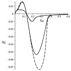
Figure 6: Comparison of the two expressions, equations (3.30) and (3.16), for $\Delta\zeta(\zeta_{0})$ for System 2. The lines with smaller $|\Delta\zeta|$ correspond to $T^{*}=0.02$; the solid line represents equation (3.16), and the dotted line represents equation (3.30). The remaining lines represent equation (3.16) (solid) and equation (3.30) (dashed) for $T^{*}=0.01$.

We first compare the change of the average volume fraction induced by mesoscopic fluctuations. The shift $\Delta\zeta$ calculated from (3.30) and (3.16) in System 1 is shown in figure 5. The shift is small for a relevant range of temperatures, and both formulas yield practically the same result — they are indistinguishable on the plot. The shift increases for a decreasing temperature. In System 2, the fluctuation contribution to the volume fraction is much larger than in System 1 (figure 5). As expected, when $\Delta\zeta$ is not very small, $\Delta\zeta/\zeta_{0}\approx 0.2$, then the two approaches yield somewhat different results, as shown in figure 6 for System 2.

In the next step, we study the chemical potential. The fluctuation contribution in System 1 is small, except at very small volume fractions (figure 7), whereas in System 2 it is substantial, and increases for decreasing temperature, as shown in figures 9 and 9. The two approaches yield similar results for small $\Delta\zeta$, whereas when $\Delta\zeta/\zeta_{0}>0.25$, significant discrepancy between the two approaches is obtained. We can conclude that on the quantitative level the approximate theory is oversimplified for the range of $T$ and $\bar{\zeta}$ for which there are significant discrepancies between the two approaches.

     

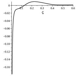
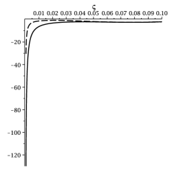
Figure 7: Left panel: the relative difference, $(\bar{\mu}-\bar{\mu}^{\mathrm{MF}})/\bar{\mu}^{\mathrm{MF}}$, between $\bar{\mu}$ calculated from equation (3.11), and the MF approximation $\bar{\mu}^{\mathrm{MF}}$ (3.12) for System 1 at $T^{*}=0.007$ and $\zeta\geqslant 0.01$. Right panel: $\bar{\mu}-\bar{\mu}^{\mathrm{MF}}$ for System 1 (solid line) and System 2 (dashed line) for $0.0005\leqslant\zeta\leqslant 0.1$.

     

Figure 8: Chemical potential in MF (dotted line), and with the fluctuation contribution included according to equation (3.11) (solid) and equation (3.27) with (3.30) (dashed line) for $T^{*}=0.015$ in System 2. The volume fraction is dimensionless, and the chemical potential is in $\pi kT/6$ units. Figure 9: Chemical potential in MF (dotted line), and with the fluctuation contribution included according to equation (3.11) (solid line), equation (3.27) with equation (3.30) (dashed line), and equation (3.27) with equation (3.16) (dashed-dotted line) for $T^{*}=0.007$ in System 2. The volume fraction is dimensionless, and the chemical potential is in $\pi kT/6$ units.

Note that since $\bar{\mu}-\bar{\mu}^{\mathrm{MF}}$ is large for volume fractions $\zeta<0.03$, for very small volume fractions our results are oversimplified.

Finally, we present the isotherms obtained from (3.24) and (3.31) for the two systems in figures 11–14. In System 1 the pressure is much higher than found in MF, and for all temperatures it monotonously increases with $\bar{\zeta}$, as shown in figure 11. The increased pressure associated with mesoscopic fluctuations may result from the repulsion between the clusters, because in this case $\tilde{V}_{\mathrm{co}}(0)>0$.

     

Figure 10: The EOS isotherms for System 1 for $T^{*}=0.02$. Dashed line is the MF result (equation (3.25)) and solid line represent equation (3.24), and equation (3.31) with equation (3.30), indistinguishable on the plot. Figure 11: The EOS isotherms (3.24) (solid line) and (3.31) with equation (3.30) (dash-dotted line), and the MF approximation (3.25) (dashed line) for System  2 for $T^{*}=0.015$.

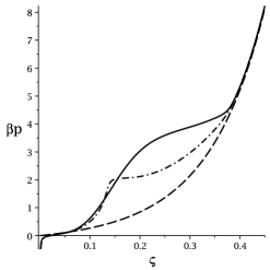
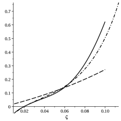
Figure 12: The EOS isotherms (3.24) (solid line) and (3.31) with equation (3.30) (dash-dotted line), and the MF approximation (3.25) (dashed line) for System 2 for $T^{*}=0.0093$. Left and right panels show large and small range of volume fractions, respectively.

     

Figure 13: The EOS isotherms (3.24) (solid line) and (3.31) with equation (3.30) (dash-dotted line), and the MF approximation (3.25) (dashed line) for System 2 for $T^{*}=0.007$. Figure 14: The EOS isotherms (3.24) (solid line) and (3.31) with equation (3.30) (dash-dotted line), and the MF approximation (3.25) (dashed line) for System 2 for $T^{*}=0.005$.

Since in System 2 $\tilde{V}_{\mathrm{co}}(0)<0$, a mechanical instability develops at the MF spinodal line, with the metastable MF critical point $T^{*}_{\mathrm{c}}\approx 0.0009$. What is really interesting is that such instability appears at much higher temperatures due to mesoscopic fluctuations. This is in strong contrast to the fluids with purely attractive interactions, where density fluctuations decrease the critical temperature with respect to the mean-field estimate. The present case with dominant fluctuations associated with mesoscopic wavelengths bears some resemblance to the restricted primitive model (RPM) of ionic systems. There is no gas-liquid instability in the RPM at the MF level of a mesoscopic theory analogous to the one considered here, but when the short-wavelength charge-density fluctuations are included, such instability appears [24]. One could imagine that the mesoscopic fluctuations, i.e., displacements of the clusters from their most probable locations lead to their coalescence when $\tilde{V}_{\mathrm{co}}(0)<0$, and thus support the phase separation. Note that properties of System 2 are completely different from the previously studied System 1.

In this region of the phase diagram, the shift of the volume fraction is large. Therefore, on the quantitative level, the results are not sufficiently accurate. The inflection point on the $P(\bar{\zeta})$ isotherm appears at $T_{\mathrm{c}}^{*}\approx 0.0093$ or $T^{*}_{\mathrm{c}}=0.007$ according to (3.31) or (3.24) with (3.30), respectively. Both temperatures, however, are much higher than in MF. Further studies are required to verify if the separation into disordered inhomogeneous phases, or periodic ordering of clusters occurs. If the ordered phases are formed, the still open question is for which part of the phase diagram such phases are globally stable.

Finally, let us focus on the pressure for very small volume fractions. In the fluctuation correction to pressure (equation (3.26)) the first term comes from the fluctuation contribution to chemical potential (see (3.11)). As shown in figure 7 (right panel), for very low volume fractions, our approximation is oversimplified, so the negative pressure is an artifact. For very low volume fractions, we should expect a perfect gas behavior, except that some fraction of particles should form clusters. Pressure should be proportional to the sum of the number densities of monomers and clusters. Since the number of clusters is smaller than the number of particles forming them, pressure should be smaller than in the corresponding perfect gas of isolated particles. Our theory agrees with this expectation (see figure 12, right panel).

5 Summary

In this work, the effects of mesoscopic fluctuations on the average volume fraction, chemical potential and pressure as functions of temperature and the average volume fraction were considered within the framework of the mesoscopic theory [5, 6]. We restricted our attention to a stable or metastable disordered phase. The fluctuation contribution to the quantities mentioned above was calculated in two ways. First, we considered the fluctuations about the average volume fraction, and derived equations (3.16), (3.11) and (3.24) for the volume fraction, chemical potential and pressure, respectively. In the second version, we considered the fluctuations about the most probable volume fraction, and obtained equations (3.30), (3.27) and (3.31), with $\zeta_{0}$ satisfying (2.12). The chemical potential and the EOS as functions of the average volume fraction are given by parametric equations (3.30) and (3.27), and (3.31), respectively. Our expressions are derived under the assumption that the dominant fluctuations are of small amplitudes. Consistent with the above assumption, the two methods yield the same result to a linear order in the fluctuation contribution to the volume fraction $\Delta\zeta$.

The fluctuation contributions to all three quantities were explicitly calculated for two versions of the SALR potential. In System 1 the zeroth moment of the effective interactions is positive and small clusters are formed. In System 2 the zeroth moment of the effective interactions is negative, and the clusters are large. We obtain nearly the same results independently of the method used when the fluctuation-induced shift of the volume fraction is very small (System 1). When $\Delta\zeta/\zeta_{0}\sim 0.2$ (low temperature in System 2), significant discrepancies between the two methods appear for some part of the phase diagram. The largest discrepancies are present when both methods yield the results that strongly deviate from the MF predictions. The larger is the probability of finding inhomogeneous mesoscopic states compared to the homogeneous distribution of particles, the stronger are the discrepancies between the two methods. It is in this part of the phase diagram that the periodic order may appear. We conclude that the first method is superior to the second one because it is easier to implement. Exact results would be necessary to get a comparison between the accuracy achieved by these methods.

We have found that mesoscopic fluctuations play a very important role and lead to a significant change of the chemical potential and pressure. The larger is the probability of finding the inhomogeneities, i.e., the further away from the structural line on the low-$T$ side of it (figure 3), the larger is the role of fluctuations. When small clusters are formed (System 1 in section 4), the fluctuation contribution to pressure increases monotonously with an increasing volume fraction. By contrast, for large clusters (System 2 in section 4) the fluctuation contribution to pressure is nonmonotonous; it is negligible for small as well as for large volume fractions, whereas for intermediate volume fractions it is large and increases with a decreasing temperature (figures 11–14). Moreover, an inflection point at the pressure – volume fraction isotherm appears at the temperature and volume fraction both much larger than found in MF. Further studies are required to verify if the periodically ordered cluster phases are stable in System 2, or phase separation occurs due to the mechanical instability. Possible scenarios are: (i) phase separation at low $T$, and periodic structures at higher $T$, or (ii) the phase separation is only metastable, and finally (iii) the periodically ordered phases are only metastable. For System 1, the phase separation is not expected.

In addition to the assumptions discussed earlier, we make an approximation concerning the form of the effective potential $V_{\mathrm{co}}$. Note that in equation (4.1) we assumed that the pair distribution function vanishes for $r<1$ in $\sigma$ units. For the volume fraction, this is a poor approximation, and quantitative results for the structural line depend on the form of the pair distribution function (regularization of the potential [27]).

In the future studies, the EOS for periodically ordered cluster phases should be determined in order to find the phase diagram. Our results indicate that despite the universal properties of the dependence of the most probable structures on the thermodynamic state, the effect of fluctuations on the average distribution of particles may depend on the form of the interaction potential, especially on the sign of the zeroth moment of the effective interactions.

Ukrainian 0

Вплив мезоскопiчних флуктуацiй на рiвняння стану кластероутворювальних систем А. Цях${}^{\textsf{\footnotesize{\mbox{?}}}}$, О. Пацаган${}^{\textsf{\footnotesize{\mbox{?}}}}$

             
${}^{\textsf{\footnotesize 1}}$ Iнститут фiзичної хiмiї, Польська академiя наук, 01-224 Варшава, Польща ${}^{\textsf{\footnotesize 2}}$ Iнститут фiзики конденсованих систем Нацiональної академiї наук України,
вул. Свєнцiцького, 1, 79011 Львiв, Україна

References

- [1] Stradner A., Sedgwick H., Cardinaux F., Poon W.C.K., Egelhaaf S.U., Schurtenberger P., Nature, 2004, 432, 492; doi:10.1038/nature03109.
-
[2]
Campbell A.I., Anderson V.J., van Duijneveldt J.S., Bartlett P.,
Phys. Rev. Lett., 2005, 94, 208301;
doi:10.1103/PhysRevLett.94.208301. - [3] Porcar L., Falus P., Chen W.-R., Faraone A., Fratini E., Hong K., Baglioni P., Liu Y., J. Phys. Chem. Lett., 2010, 1, 126; doi:10.1021/jz900127c.
- [4] Stiakakis E., Petekidis G., Vlassopoulos D., Likos C.N., Iatrou H., Hadjichristidis N., Roovers J., Europhys. Lett., 2005, 72, 664; doi:10.1209/epl/i2005-10283-y.
- [5] Ciach A., Phys. Rev. E, 2008, 78, 061505; doi:10.1103/PhysRevE.78.061505.
- [6] Ciach A., Mol. Phys., 2011, 109, 1101; doi:10.1080/00268976.2011.638329.
- [7] Sear R.P., Gelbart W.M., J. Chem. Phys., 1999, 110, 4582; doi:10.1063/1.478338.
- [8] Archer A.J., Wilding N.B., Phys. Rev. E, 2007, 76, 031501; doi:10.1103/PhysRevE.76.031501.
- [9] Archer A.J., Pini D., Evans R., Reatto L., J. Chem. Phys., 2007, 126, 014104; doi:10.1063/1.2405355.
- [10] Archer A.J., Phys. Rev. E, 2008, 78, 031402; doi:10.1103/PhysRevE.78.031402.
- [11] Ciach A., Góźdź W.T., Condens. Matter Phys., 2010, 13, 23603; doi:10.5488/CMP.13.23603.
- [12] De Candia A., Del Gado E., Fierro A., Sator N., Tarzia M., Coniglio A., Phys. Rev. E, 2006, 74, 010403(R); doi:10.1103/PhysRevE.74.010403.
-
[13]
Kowalczyk P., Ciach A., Gauden P.A., Terzyk A.P., J. Colloid Interface Sci.,
2011, 363, 579;
doi:10.1016/j.jcis.2011.07.043. -
[14]
Sciortino F., Mossa S., Zaccarelli E., Tartaglia P., Phys. Rev.
Lett., 2004, 93, 055701;
doi:10.1103/PhysRevLett.93.055701. - [15] Sciortino F., Tartaglia P., Zaccarelli E., J. Phys. Chem. B, 2005. 109, 21942; doi:10.1021/jp052683g.
- [16] Toledano J., Sciortino F., Zaccarelli E., Soft Matter, 2009, 5, 2390; doi:10.1039/b818169a.
- [17] Shukla A., PNAS, 2008, 105, 5075; doi:10.1073/pnas.0711928105.
- [18] Zhang T.H., Groenewold J., Kegel W.K., Phys. Chem. Chem. Phys., 2009, 11, 10827; doi:10.1039/b917254h.
- [19] Ciach A., Góźdź W.T., Stell G., J. Phys.: Condens. Matter, 2006, 18, 1629; doi:10.1088/0953-8984/18/5/016.
- [20] Evans R., Adv. Phys., 1979, 28, 143l doi:10.1080/00018737900101365.
- [21] Patsahan O., Ciach A., J. Phys.: Condens. Matter, 2007, 19, 236203; doi:10.1088/0953-8984/19/23/236203.
- [22] Brazovskii S.A., Sov. Phys. JETP, 1975, 41, 85.
- [23] Ciach A., Patsahan O., Phys. Rev. E, 2006, 74, 021508; doi:10.1103/PhysRevE.74.021508.
- [24] Ciach A., Stell G., J. Mol. Liq., 2000, 87, 255; doi:10.1016/S0167-7322(00)00125-2.
- [25] Ciach A, Góźdź W.T., Evans R, J. Chem. Phys., 2003, 118, 3702; doi:10.1063/1.1539046.
- [26] Stell G., In: New Approaches to Problems in Liquid-State Theory, edited by C. Caccamo, J.-P. Hansen, and G. Stell, Kluwer Academic Publishers, Dordrecht, 1999.
- [27] Patsahan O.V., Mryglod I.M., Condens. Matter Phys., 2004, 7, 755.
Ukrainian \adddialect\l@ukrainian0 \l@ukrainian