Temperature dependence of the paramagnetic spin susceptibility of doped graphene

Abstract

In this work, we present a semi-analytical expression for the temperature dependence of a spin-resolved dynamical density-density response function of massless Dirac fermions within the Random Phase Approximation. This result is crucial in order to describe thermodynamic properties of the interacting systems. In particular, we use it to make quantitative predictions for the paramagnetic spin susceptibility of doped graphene sheets. We find that, at low temperatures, the spin susceptibility behaves like $T^{-2}$ which is completely different from the temperature dependence of the magnetic susceptibility in undoped graphene sheets.

I Introduction

Graphene is a newly realized two-dimensional (2D) electron system that has attracted a great deal of interest because of the new physics which it exhibits and because of its potential as a new material for electronic technology reviews ; PT . It exhibits a large number of new and exotic optical and electronic effects that have not been observed in other materials nair .

When non-relativistic Coulombic electron-electron interactions are added to the kinetic Hamiltonian, graphene represents a new type of many-electron problem, distinct from both an ordinary 2D electron gas (EG) and from quantum electrodynamics. The Dirac-like wave equation and the chirality of its eigenstates lead indeed to both unusual electron-electron interaction effects bostwick ; diracgaspapers ; barlas_prl_2007 ; polini_ssc_2007 ; polini_prb_2008 ; dassarmadgastheory and an unusual response to external potentials tomadin_prb_2008 ; rossi_prl_2008 .

Spin transport of fermions is central to many fields of physics. Electron transport runs modern technology and electron spin is being explored as a new carrier of information wolf . There has been recent interest in the temperature dependence of various Fermi liquid properties 2d-transport . Technical advances now allow one to measure the temperature dependence of the thermodynamic and transport parameters such as conductivity at finite temperature in unsuspended morozov_prl_2008 ; chen_nature_nanotech_2008 , and suspended graphene sheets bolotin_prl_2008 ; du_nature_nanotech_2008 and spin susceptibility in two-dimensional systems.

The paramagnetic spin susceptibility shows behavior similar to the charge compressibility barlas_prl_2007 which decreases as the interaction increases at zero temperature. This is related to the fact that the inverse of the spin susceptibility is proportional to the renormalized Fermi velocity.

Vafek vafek_prl_2007 has recently shown that the specific heat of undoped graphene sheets presents an anomalous low-temperature behavior displaying a logarithmic suppression with respect to its noninteracting counterpart as $\sim T/\ln(T)$. Meanwhile, Sheery and Schmalian studied both the specific heat and the orbital diamagnetic susceptibility of undoped graphene by using a renormalization group approach sheehy . They stated that the dependence of the diamagnetic susceptibility of undoped graphene on temperature is quite different from the 2D EGs and it behaves like $T/|\ln(T)|^{2}$.

On the other hand, it has been demonstrated in Refs. polini_ssc_2007 ; polini_prb_2008 (see also Ref. dassarmadgastheory ) that doped graphene sheets are normal (pseudochiral) Fermi liquids, with Landau parameters that possess a behavior quite distinct from that of conventional 2D EGs. In addition, it was found that ramezan , at low temperatures, the specific heat has the usual normal-Fermi-liquid linear-in-temperature behavior, with a slope that is solely controlled by the renormalized quasiparticle velocity in doped graphene.

The temperature correction to the spin susceptibility for a 2D EG interacting via a long-range Coulomb interaction has attracted a lot of interest over a long period of time 2d . It has been shown that the dynamic Kohn anomaly in the density-density response function at $2k_{\rm F}$ and re-scattering of pairs of quasiparticles lead to linear-in-temperature correction to the spin susceptibility theory_2d . Since the static non-interacting density-density response function of doped graphene is a smooth function at $2k_{\rm F}$ and behaves differently from what one has in standard 2D EG systems, a linear-in-temperature correction to the spin susceptibility does not occur.

In this work we calculate the temperature dependence of a spin-resolved dynamical density-density response function of massless Dirac fermions within the Random Phase Approximation (RPA) and subsequently the Helmholtz free energy ${\cal F}(T)$ of doped graphene sheets where the chemical potential is non zero. This allows us to access important thermodynamic quantities, such as the spin susceptibility which can be calculated by taking appropriate derivatives of the free energy. We show that, at low temperatures, the spin compressibility of doped graphene, in contrary to the diamagnetic spin susceptibility sheehy , behaves as the inverse square of temperature, solely controlled by both the ultraviolet cut-off and graphene’s fine-structure constant.

In Sec. II we introduce the formalism that will be used in calculating (paramagnetic) spin susceptibility which includes the many-body effects in the RPA. In Sec. III we present our analytical and numerical results for the free energy and spin susceptibility in doped graphene sheets. Sec. V contains discussions and conclusions.

II METHOD AND THEORY

The agent responsible for many of the interesting electronic properties of graphene sheets is the non-Bravais honeycomb-lattice arrangement of carbon atoms, which leads to a gapless semiconductor with valence and conduction $\pi$-bands. States near the Fermi energy of a graphene sheet are described by a spin-independent massless Dirac Hamiltonian slonczewski

$${\cal H}=v_{\rm F}{\bm{\sigma}}\cdot{\bm{p}}~{},$$ (1)

where $v_{\rm F}$ is the Fermi velocity, which is density-independent and roughly three-hundred times smaller that the velocity of light in vacuum, and ${\bm{\sigma}}=(\sigma^{x},\sigma^{y})$ is a vector constructed with two Pauli matrices $\{\sigma^{i},i=x,y\}$, which operate on pseudospin (sublattice) degrees of freedom. Note that the eigenstates of ${\cal H}$ have a definite chirality rather than a definite pseudospin, i.e. they have a definite projection of the honeycomb-sublattice pseudospin onto the momentum ${\bm{p}}$.

Electrons in graphene do not move around as independent particles. Rather, their motions are correlated due to pairwise Coulomb interactions. The interaction potential is sensitive to the dielectric media surrounding the graphene sheet. The Fourier transform of the real space potential is given by $v_{q}=2\pi e^{2}/\epsilon q$ where $\epsilon$ is the average dielectric constant between the medium and a dielectric constant of the substrate.

Within this low energy description, the properties of doped graphene sheets depend on the dimensionless coupling constant or graphene’s fine-structure constant

$$\alpha_{\rm ee}=\frac{e^{2}}{\epsilon\hbar v_{\rm F}}~{}.$$ (2)

As it is clearly seen from Eq. (1), the spectrum is unbounded from below and it implies that the Hamiltonian has to be accompanied by an ultraviolet cut-off which is defined $k_{\rm c}$ and it should be assigned a value corresponding to the wavevector range over which the continuum model Eq. (1) describes graphene. For later purposes we define $\alpha_{\rm gr}=2g_{\rm v}\alpha_{\rm ee}$ where $g_{\rm v}=2$ accounts for valley degeneracy, $k^{\sigma}_{\rm F}=k_{\rm F}(1+\zeta\sigma)^{1/2}$ is the spin dependent Fermi momentum and $k_{\rm F}=(\pi n)^{1/2}$ is the Fermi wave number and $\varepsilon_{\rm F}=\hbar v_{\rm F}k_{\rm F}$ is being the Fermi energy with $n=n^{\uparrow}+n^{\downarrow}$ the total electron density, $\zeta=(n^{\uparrow}-n^{\downarrow})/n$ is the spin polarization parameter (0 $\leq\zeta\leq$ 1 if we assume that, e. g., electrons with real spin $s=\uparrow$ to be majority). For definiteness we take $k_{\rm c}$ to be such that $\pi k^{2}_{\rm c}=2(2\pi)^{2}/{\cal A}_{0}$, where ${\cal A}_{0}=3\sqrt{3}a^{2}_{0}/2$ is the area of the unit cell in the honeycomb lattice, with $a_{0}\simeq 1.42$ Å the Carbon-Carbon distance. With this choice, the energy $\hbar vk_{c}=7$ eV and

$$\Lambda=\frac{k_{\rm c}}{k_{\rm F}}=\sqrt{\frac{2g_{\rm v}}{n{\cal A}_{0}}}~{}.$$ (3)

The continuum model is useful when $k_{\rm c}\gg k_{\rm F}$, i.e. when $\Lambda\gg 1$. Note that, for instance, electron densities $n=0.36\times 10^{12}$ and $0.36\times 10^{14}$ cm^-2 correspond to $\Lambda=100$ and $10$, respectively.

The free energy ${\cal F}={\cal F}_{0}+{\cal F}_{\rm int}$, a thermodynamic potential at a constant temperature and volume, is usually decomposed into the sum of a noninteracting term ${\cal F}_{0}$ and an interaction contribution ${\cal F}_{\rm int}$. To evaluate the interaction contribution to the Helmholtz free energy we follow a familiar strategy Pines_and_Nozieres ; Giuliani_and_Vignale by combining a coupling constant integration expression for ${\cal F}_{\rm int}$ valid for uniform continuum models ($\hbar=1$ from now on),

$${\cal F}_{\rm int}(T)=\frac{N}{2}\int_{0}^{1}d\lambda\int\frac{d^{2}{\bm{q}}}{(2\pi)^{2}}v_{q}\left[S^{(\lambda)}(q,T)-1\right]~{},$$ (4)

with a fluctuation-dissipation-theorem (FDT) expression Giuliani_and_Vignale for the static structure factor,

$$S^{(\lambda)}(q,T)=-\frac{1}{\pi n}\int_{0}^{+\infty}d\omega~{}\coth{(\beta\omega/2)}\Im m\chi^{(\lambda)}_{\rho\rho}(q,\omega,T)~{}.$$ (5)

Here $\beta=(k_{\rm B}T)^{-1}$. Quite generally, two-particle correlation functions can be written in terms of single-particle Green s functions and vertex parts. The RPA approximation for ${\cal F}_{\rm int}$ then follows from the RPA approximation for $\chi^{(\lambda)}_{\rho\rho}(q,\omega)$:

$$\chi^{(\lambda)}_{\rho\rho}(q,\omega,T)=\frac{\chi^{\uparrow}_{0}(q,\omega,T)+\chi^{\downarrow}_{0}(q,\omega,T)}{1-\lambda v_{q}(\chi^{\uparrow}_{0}(q,\omega,T)+\chi^{\downarrow}_{0}(q,\omega,T))}$$ (6)

where $\chi^{\sigma}_{0}(q,\omega,T)$ is the noninteracting spin resolved density-density response-function in $\sigma$ channel. A central quantity in the many-body techniques is the noninteracting spin resolved polarizability function $\chi^{\sigma}_{0}(q,\omega,T)$ . The problem of linear density response is set up by considering a fluid described by the Hamiltonian, which is subject to an external potential. The external potential must be sufficiently weak for low-order perturbation theory to suffice. The induced density change has a linear relation to the external potential through the noninteracting dynamical polarizability function. This function in $\sigma$ channel reads as

$$\chi^{\sigma}_{0}(q,\omega,T) = g_{\rm v}\lim_{\eta\to 0^{+}}\sum_{s,s^{\prime}=\pm}\int\frac{d^{2}{\bm{k}}}{(2\pi)^{2}}\frac{1+ss^{\prime}\cos(\theta_{{\bm{k}},{\bm{k}}+{\bm{q}}})}{2}$$ (7)

$$\times \frac{n^{\sigma}_{\rm F}(\varepsilon_{{\bm{k}},s})-n^{\sigma}_{\rm F}(\varepsilon_{{\bm{k}}+{\bm{q}},s^{\prime}})}{\omega+\varepsilon_{{\bm{k}},s}-\varepsilon_{{\bm{k}}+{\bm{q}},s^{\prime}}+i\eta}~{}.$$

Here $\varepsilon_{{\bm{k}},s}=sv_{\rm F}k$ are the Dirac band energies and $n^{\sigma}_{\rm F}(\varepsilon)=\{\exp[\beta(\varepsilon-\mu^{\sigma}_{0})]+1\}^{-1}$ is the usual Fermi-Dirac distribution function, $\mu^{\sigma}_{0}=\mu^{\sigma}_{0}(T)$ being the noninteracting chemical potential. As usual, this is determined by the normalization condition

$$n^{\sigma}=\int_{-\infty}^{+\infty}d\varepsilon~{}\nu(\varepsilon)n^{\sigma}_{\rm F}(\varepsilon)~{},$$ (8)

where $\nu(\varepsilon)=g_{\rm v}\varepsilon/(2\pi v^{2}_{\rm F})$ is the noninteracting density of states. For $T\to 0$ one finds $\mu^{\sigma}_{0}(T)=\varepsilon^{\sigma}_{\rm F}\{1-\pi^{2}(T/T_{\rm F})^{2}/6(1+\sigma\zeta)\}$, where $T_{\rm F}=\varepsilon_{\rm F}/k_{B}$ is the Fermi temperature. The factor in the first line of Eq. (7), which depends on the angle $\theta_{{\bm{k}},{\bm{k}}+{\bm{q}}}$ between ${\bm{k}}$ and ${\bm{k}}+{\bm{q}}$, describes the dependence of Coulomb scattering on the relative chirality $ss^{\prime}$ of the interacting electrons.

After some straightforward algebraic manipulations ramezan we arrive at the following expressions for the imaginary, $\Im m~{}\chi^{\sigma}_{0}$, and the real, $\Re e~{}\chi^{\sigma}_{0}$, parts of the noninteracting density-density response function for $\omega>0$:

$$\Im m~{}\chi^{\sigma}_{0}(q,\omega,T)=\frac{g_{\rm v}}{4\pi}\sum_{\alpha=\pm}\Bigg{\{}\Theta(v_{\rm F}q-\omega)q^{2}f(v_{\rm F}q,\omega)$$

$$\times \left[G^{(\alpha,\sigma)}_{+}(q,\omega,T)-G^{(\alpha,\sigma)}_{-}(q,\omega,T)\right]$$

$$+ \Theta(\omega-v_{\rm F}q)q^{2}f(\omega,v_{\rm F}q)\left[-\frac{\pi}{2}\delta_{\alpha,-}+H^{(\alpha,\sigma)}_{+}(q,\omega,T)\right]\Bigg{\}}$$

and

$$\Re e~{}\chi^{\sigma}_{0}(q,\omega,T)=\frac{g_{\rm v}}{4\pi}\sum_{\alpha=\pm}\Bigg{\{}\frac{-2k_{\rm B}T\ln[1+e^{\alpha\mu_{0}/(k_{\rm B}T)}]}{v^{2}_{\rm F}}$$

$$+ \Theta(\omega-v_{\rm F}q)q^{2}f(\omega,v_{\rm F}q)\left[G^{(\alpha,\sigma)}_{-}(q,\omega,T)-G^{(\alpha,\sigma)}_{+}(q,\omega,T)\right]$$

$$+ \Theta(v_{\rm F}q-\omega)q^{2}f(v_{\rm F}q,\omega)\left[-\frac{\pi}{2}\delta_{\alpha,-}+H^{(\alpha,\sigma)}_{-}(q,\omega,T)\right]\Bigg{\}}~{}.$$

Here

$$f(x,y)=\frac{1}{2\sqrt{x^{2}-y^{2}}}~{},$$ (11)

$$G^{(\alpha,\sigma)}_{\pm}(q,\omega,T)=\int_{1}^{\infty}du~{}\frac{\sqrt{u^{2}-1}}{\exp\left({\displaystyle\frac{|v_{\rm F}qu\pm\omega|-2\alpha\mu^{\sigma}_{0}}{2k_{\rm B}T}}\right)+1}~{},$$ (12)

and

$$H^{(\alpha,\sigma)}_{\pm}(q,\omega,T)=\int_{-1}^{1}du~{}\frac{\sqrt{1-u^{2}}}{\exp\left({\displaystyle\frac{|v_{\rm F}qu\pm\omega|-2\alpha\mu^{\sigma}_{0}}{2k_{\rm B}T}}\right)+1}~{}.$$ (13)

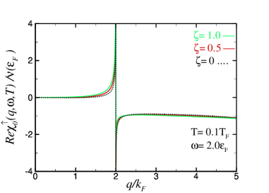
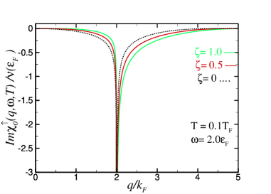
Figure 1: ( Color online) Upper : the real part of the dynamical response function $\Re e~{}\chi^{\uparrow}_{0}(q,\omega,T)$ [in units of $\nu(\varepsilon_{\rm F})$] as a function of $q/k_{\rm F}$ for $\omega=2\varepsilon_{\rm F}$, $T=0.1T_{\rm F}$ and three values of $0\leq\zeta\leq 1$. Bottom: same as in the upper panel but for the imaginary part.

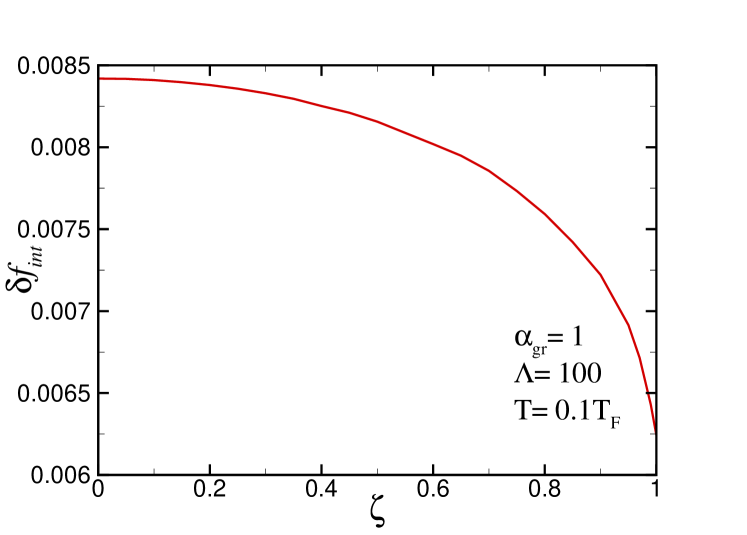
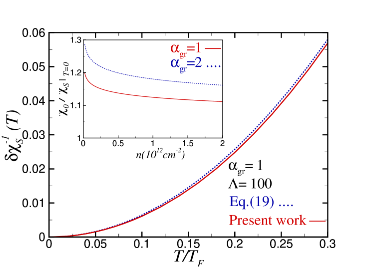
Figure 2: (Color online) Upper: $\delta f_{\rm int}$ in units of $\varepsilon_{\rm F}$ as a function of spin polarization parameter, $\zeta$ for $\alpha_{\rm gr}=1$ and $T=0.1T_{\rm F}$. Bottom : Numerical calculated $\delta\chi^{-1}_{s}(T)=\chi^{-1}_{s}(T)-\chi^{-1}_{s}(T=0)$ in units of $\varepsilon_{\rm F}/n\mu_{B}^{2}$ as a function of temperature for $\alpha_{gr}=1$ in comparison with the low temperature approximated expression given by Eq.(19). These numerical results confirm the validity of our analytic result for $\delta f_{\rm int}$. In the inset, the inverse spin susceptibility scaled by non-interacting one as a function of electron density in units of $10^{12}$ cm^-2 at zero temperature for different $\alpha_{gr}$ values.

The coupling constant integration in Eq. (4) can be carried out partly analytically due to the simple RPA expression Eq. (6). We find that the interaction contribution to the free energy per particle $f_{\rm int}(T)$ is given by

$$f_{\rm int}(T)=\frac{1}{2}\int\frac{d^{2}{\bm{q}}}{(2\pi)^{2}}\left\{-\frac{1}{\pi n}\int_{0}^{+\infty}d\omega\coth{(\beta\omega/2)}\times\right.$$ (14)

$$\left.\arctan\left[\frac{v_{q}[\Im m~{}\chi^{\uparrow}_{0}+\Im m~{}\chi^{\downarrow}_{0}]}{1-v_{q}[\Re e~{}\chi^{\uparrow}_{0}+\Re e~{}\chi^{\downarrow}_{0})]}\right]-v_{q}\right\}$$

$$+ \frac{1}{2n}\int\frac{d^{2}{\bm{q}}}{(2\pi)^{2}}\int_{0}^{1}\frac{d\lambda}{\lambda}\coth{(\beta\omega_{\rm pl}/2)}[\Re e~{}\chi^{\uparrow}_{0}+\Re e~{}\chi^{\downarrow}_{0}]$$

$$\times \left|{\frac{\partial[\Re e~{}\chi^{\uparrow}_{0}+\Re e~{}\chi^{\downarrow}_{0}]}{\partial\omega}}\right|^{-1}_{\omega=\omega_{\rm pl}}\,.$$

In this equation the first term comes from the smooth electron-hole contribution to $\Im m~{}\chi^{(\lambda)}_{\rho\rho}$, while the second term comes from the plasmon contribution; $\omega^{\sigma}_{\rm pl}=\omega_{\rm pl}(q,T,\lambda)$ is the plasmon dispersion relation at coupling constant $\lambda$ which can be found numerically by solving the equation $1-\lambda v_{q}\Re e~{}\chi^{\sigma}_{0}(q,\omega,T)=0$. Note that in a standard 2D EG the exchange energy starts to matter little for $T$ of order $T_{\rm F}$ because all the occupation numbers are small and the Pauli exclusion principle matters little. In the graphene case however exchange interactions with the negative energy sea remain important as long as $T$ is small compared to $v_{\rm F}k_{\rm c}/k_{\rm B}=T_{\rm F}\Lambda$.

The free energy calculated according to Eq. (14) is divergent since it includes the interaction energy of the model’s infinite sea of negative energy particles. Following Vafek vafek_prl_2007 , we choose the free energy at $T=0$, $f(T=0)$, as our “reference” free energy, and thus introduce the regularized quantity $\delta f\equiv f(T)-f(T=0)$. This again can be decomposed into the sum of a noninteracting contribution, $\delta f_{0}(T\to 0)=-g_{v}\varepsilon_{\rm F}\pi^{2}(T/T_{\rm F})^{2}Z(\zeta,1/2)/12$, where $Z(\zeta,m)=(1+\zeta)^{m}+(1-\zeta)^{m}$ and an interaction-induced contribution $\delta f_{\rm int}(T)=f_{\rm int}(T)-f_{\rm int}(T=0)$, which can be calculated from Eq. (14). Note that we have $f_{0}(T=0)=g_{v}\varepsilon_{\rm F}Z(\zeta,3/2)/6$.

The low-temperature behavior of the interaction contribution to the free energy can be extracted analytically with some patience. After some lengthy but straightforward algebra we find, to leading order in $\Lambda$,

$$\delta f_{\rm int}(T\to 0)=\varepsilon_{\rm F}\frac{\pi^{2}}{6}\left(\frac{T}{T_{\rm F}}\right)^{2}\frac{\alpha_{\rm gr}[1-\alpha_{\rm gr}\xi(\alpha_{\rm gr})]}{8g_{\rm v}}$$

$$\times Z(\zeta,1/2)\ln{\Lambda}+{\rm R.~{}T.}$$ (15)

where the function $\xi(x)$, defined as in Eq. (14) of Ref. [polini_ssc_2007, ], is given by $\xi(x)=128/(\pi^{2}x^{3})-32/(\pi^{2}x^{2})+1/x-h(\pi x/8)$, with

$$h(x)=\left\{\begin{array}[]{ll}{\displaystyle\frac{1}{2x^{3}\sqrt{1-x^{2}}}\arctan{\left(\frac{\sqrt{1-x^{2}}}{x}\right)}}&{\displaystyle{\rm for}~{}x<1\vspace{0.1 cm}}\\ {\displaystyle\frac{1}{4x^{3}\sqrt{x^{2}-1}}\ln{\left(\frac{x+\sqrt{x^{2}-1}}{x-\sqrt{x^{2}-1}}\right)}}&{\displaystyle{\rm for}~{}x>1}\end{array}\right.\,.$$ (16)

The symbol ${\rm R.~{}T.}$ in the l.f.s. of Eq. (II) indicates regular terms, i.e. terms that, by definition, are finite in the limit $\Lambda\to\infty$. Eq. (II) represents the second important result of this work.

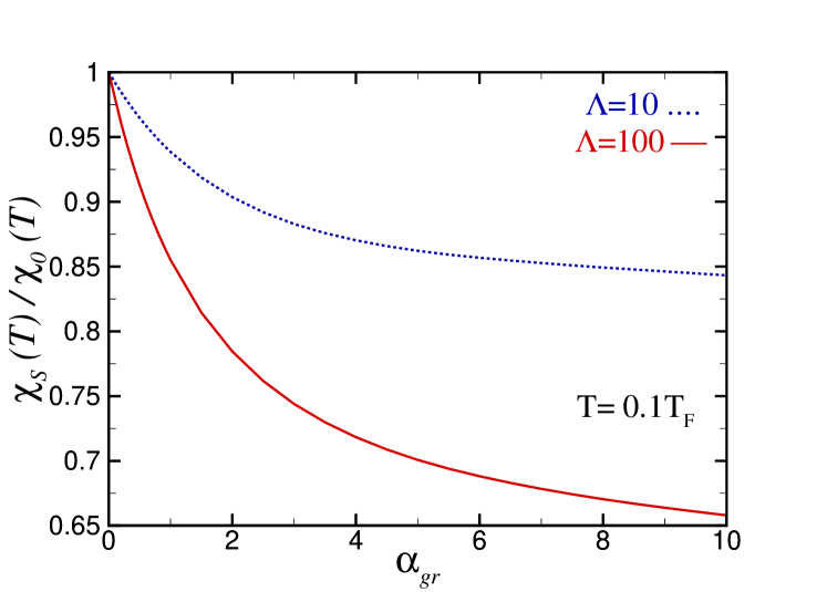
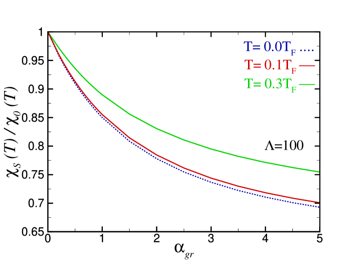
Figure 3: (Color online) Upper: the spin susceptibility (in units of the non-interacting spin susceptibility $\chi_{0}$) as a function of coupling constant for two values of ultraviolet cut-off, $\Lambda=10$ and $100$. The spin susceptibility decreases with increasing $\Lambda$ or the coupling constant. Bottom: the same as upper panel for three values of temperature for $\Lambda=100$.

We thus see that $\delta f_{\rm int}(T\to 0)\propto T^{2}$ in Eq. (II) implies a conventional Fermi-liquid behavior with a linear-in-$T$ specific heat. We are thus led to conclude, in full agreement with the zero-temperature calculations of the quasiparticle energy and lifetime performed in Refs. polini_ssc_2007 ; polini_prb_2008 , that doped graphene sheets are normal Fermi liquids.

It would be worthwhile obtaining the high-temperature dependence of $\delta f$. Since we are always measuring energies in units of the Fermi energy, therefore our high energy results are relevant to Dirac point physics. The undoped limit for us is the limit of vanishing the Fermi energy. To obtain the results for undoped graphene, let’s consider the paramagnetic case. By replacing the Fermi energy with $k_{\rm B}T$ and therefore, $k_{\rm F}$ with $k_{\rm B}T/\hbar v_{\rm F}$ in Eq. II, the correction to the free-energy is given by $\delta f_{\rm int}(T\gg T_{\rm F},n\simeq 0)\sim T^{3}\alpha_{gr}[1-\alpha_{gr}\xi(\alpha_{gr})]\ln(k_{c}/T)/(8g_{v})$. Importantly, this expression, apart from a constant note , is coincide with that result obtained in Eq. 13 by Vafek vafek_prl_2007 . Therefore, we expect that in the limit that $T\gg T_{\rm F}$ and for every $\zeta$ value, the temperature dependence of the free-energy correction behaves like $T^{3}\ln(k_{c}/T)$.

The spin susceptibility, on the other hand, can be calculated from the second derivative of the Helmholtz free energy and it reads

$$\frac{1}{\chi_{s}(T)}=\frac{1}{n\mu^{2}_{B}}\frac{\partial^{2}[f_{0}(T,\zeta)+f_{\rm int}(T,\zeta)]}{\partial\zeta^{2}}~{}|_{\zeta=0}~{},$$ (17)

where $\mu_{B}$ is the Bohr magneton footnote .

It is easy to calculate the non-interaction spin susceptibility and it turns out that

$$\chi_{0}^{-1}(T)=\frac{1}{n\mu^{2}_{B}}\frac{g_{v}\varepsilon_{\rm F}}{4}\{1+\frac{\pi^{2}}{6}(\frac{T}{T_{\rm F}})^{2}\}~{}.$$ (18)

At low temperature, by using $\delta f_{\rm int}$ to leading order in $\Lambda$, the temperature dependence of the correction to the spin susceptibility is thus given by

$$\delta\chi_{s}^{-1}(T) = \chi^{-1}_{s}(T)-\chi^{-1}_{s}(T=0)$$ (19)

$$= \frac{\varepsilon_{\rm F}\pi^{2}}{8n\mu_{B}^{2}}(\frac{T}{T_{\rm F}})^{2}\left[\frac{g_{v}}{3}-\eta\ln\Lambda\right]$$

where $\eta=\alpha_{gr}(1-\alpha_{gr}\xi(\alpha_{gr}))/12g_{v}$. It is obvious from the expression that $\chi_{s}(T)\propto T^{-2}$ at low temperature limit. This expression represents our important result in this work.

III NUMERICAL RESULTS

In this section, we present the most important results of the spin susceptibility in doped graphene sheets by using mentioned formalism.

The semi-analytical expressions for $\Re e~{}\chi^{\sigma}_{0}(q,\omega,T)$ and $\Im m~{}\chi^{\sigma}_{0}(q,\omega,T)$ constitute the first important result of this work. In Fig. 1 we have plotted the major part of the dynamic response function as a function of $q/k_{\rm F}$ for different values of $\zeta$. Sharp cutoffs in the imaginary part of $\chi^{\uparrow}_{0}(q,\omega,T)$ are related to the rapid swing in the real part of $\chi^{\uparrow}_{0}(q,\omega,T)$. These behaviors are in result of the fact that the real and imaginary parts of the polarization function are related through the Kramers-Krönig relations. Importantly, the sign change of the real part from negative to positive shows a sweep across the electron-hole continuum. It is important to note that there is a non-monotonic behavior of $\chi^{\sigma}_{0}(q,0,T)$ as a temperature dependent originates from a competition between intra- and inter-band contributions to this quantity ramezan . However, the spin polarization parameter dependence of the Lindhard function is a monotonic behavior at any frequency.

Fig. 2 (upper) shows the interaction contributions of the free energy as a function of spin polarization for $T=0.1T_{\rm F}$. Our numerical results show that the contribution of electron-electron interactions in the free energy decrease by increasing the spin polarization. It changes slightly at low $\zeta$ values and sharply decreases near the ferromagnetic case. The reason is that the exchange and correlation energies mostly change around the fully ferromagnetic point. Moreover, the slope of exchange and correlation energies with respect to $\zeta$ around $\zeta=1$ have opposite signs QA and the interaction contribution tends to the correlation sign at certain value of $\zeta$. Fig. 2 (bottom) shows the numerical calculated $\chi^{-1}_{s}(T)-\chi^{-1}_{s}(T=0)$ as a function of temperature in comparison with that result obtained at low temperature and leading order of $\Lambda$. We can easily see that those results are very close at low temperature and confirm that the spin susceptibility behaves as $T^{-2}$ in this region. In addition, this comparison allows us to use the approximated analytical expression given by Eq. (19) for the temperature correction of the spin susceptibility till $T\leq 0.3T_{\rm F}$. Furthermore, we can see that the spin susceptibility sharply decreases with increasing temperature. On the other hand, temperature dependence of the spin susceptibility is in contrast to that result obtained for the diamagnetic undoped graphene sheet. To seek comprehensive study, we have numerically calculated $\chi_{0}/\chi_{s}$ as a function of electron density in units of $10^{12}$ cm^-2 at zero temperature, $T=0$. Our results are shown in the inset of Fig. 2 (bottom) and show that the spin susceptibility increases by increasing the electron density barlas_prl_2007 .

Finally, we show the spin susceptibility scaled by its non-interacting value as a function of the coupling constant for (upper panel) two values of the ultraviolet cut-off and (bottom panel) different values of temperatures in Fig. 3. These results are obtained numerically by taking the full terms of Eq. (14). We can clearly see that the spin susceptibility increases by increasing the electron density ( or decreasing the $\Lambda$ values) while it decreases by increasing the interactions at certain temperature value. The reason is that the exchange contribution term makes a positive contribution to Eq. (18), thus tending to reduce the spin susceptibility (with respect to its noninteracting value), again in contrast to what happens in the standard 2D EG where exchange enhances the spin susceptibility. The correlation term instead makes a negative contribution to Eq. (18), thus tending to enhance the spin susceptibility. In the 2D EG, correlations tend to reduce the spin susceptibility.

IV Conclusions

We have presented semi-analytical expressions for the real and the imaginary parts of the resolved spin dependence of density-density linear-response function of noninteracting massless Dirac fermions at finite temperature. These results are very useful in order to study finite-temperature screening within the Random Phase Approximation. For example they can be used to calculate the spin dependence of the conductivity at finite temperature within Boltzmann transport theory .

The Lindhard function at finite temperature is also extremely useful to calculate finite-temperature equilibrium properties of interacting massless Dirac fermions, such as the specific heat and the compressibility. For example, in this work we have been able to show that, at low temperatures, the paramagnetic spin susceptibility of interacting massless Dirac fermions behaves like $T^{-2}$ at low temperature. Even though the charge and spin susceptibilities behave similarly at zero temperature, their temperature dependencies are totally different. We have obtained an analytical expression for the spin susceptibility in the leading order of cut-off and showed that one can use that in the low temperature range for experimental access.

We remark that in a very small density region, the system is highly correlated and a model going beyond the RPA is necessary to account for increasing correlation effects at low density.

V Acknowledgement

We thank A. Naji for his useful comments. We would like to dedicate this report to the memory of my sister, ” Farideh Asgari”.

References

- (1) A. K. Geim and K. S. Novoselov, Nature Mater. 6 183 (2007); Exploring graphene — Recent research advances, Solid State Comminu. 143 (2007), edited by S. Das Sarma, A. K. Geim , P. Kim , A. H. and MacDonald; A. H. Castro Neto, F. Guinea, N. M. P. Peres, K. S. Novoselov and A. K. Geim, Rev. Mod. Phys. 81, 109 (2009) .
- (2) For a recent popular review see A. K. Geim and A. H. MacDonald, Phys. Today 60 35 (2009) .
- (3) R. R. Nair, P. Blake, A. N. Grigorenko, K. S. Novoselov, T. J. Booth, T. Stauber, N. M. R. Peres, and A. K. Geim ,Science 320, 1308 (2008); N. Levy, S. A. Burke, K. L. Meaker, M. Panlasigui, A. Zettl, F. Guinea, A. H. Castro Neto, and M. F. Crommie, Science 329, 544 (2010) .
- (4) Aaron Bostwick, Florian Speck, Thomas Seyller, Karsten Horn, Marco Polini, Reza Asgari, Allan H. MacDonald, and Eli Rotenberg, Science, 328, 999 (2010) .
- (5) J. González, F. Guinea and M. A. H. Vozmediano, Phys. Rev. Lett. bf 77 3589 (1996); J. Gonzáles, F. Guinea and M. A. H. Vozmediano, Phys. Rev. B, 59 R2474 (1999) .
- (6) Y. Barlas, T. Pereg-Barnea, M. Polini, R. Asgari and A. H. MacDonald, Phys. Rev. Lett. 98, 236601 (2007) .
- (7) M. Polini, R. Asgari, Y. Barlas, T. Pereg-Barnea and A. H. MacDonald, Solid State Commiun. 143 58, (2007) .
- (8) M. Polini, R. Asgari, G. Borghi, Y. Barlas, T. Pereg-Barnea and A. H. MacDonald, Phys. Rev. B, 77 081411(R)(2008); A. Qaiumzadeh, R. Asgari, Phys. Rev. B 79, 075414 (2009); ibid, New J. Phys. 11 , 095023 (2010) .
- (9) A. Qaiumzadeh, N. Arabchi and R. Asgari , Solid State Comminu. 147, 172 (2008); E. H. Hwang and S. Das Sarma, Phys. Rev. B 75, 205418 (2007); S. Das Sarma, E. H. Hwang and W-K Tse, Phys. Rev. B 75, 121406(R) (2007); R. Asgari, M. M. Vazifeh, M. R. Ramezanali, E. Davoudi and B. Tanatar Phys. Rev. B 77 , 125432 (2008) .
- (10) M. Polini , A. Tomadin, R. Asgari and A. H. MacDonald Phys. Rev. B, 78, 115426 (2008) .
- (11) E. Rossi and S. Das Sarma, Phys. Rev. Lett. 101, 166803 (2008) .
- (12) S. A. Wolf, Science 294, 1488 (2001) .
- (13) D. Belitz, T. R. Kirkpatrick, and T. Vojta, Phys. Rev. B 55, 9452 (1997); S. Das Sarma, V. M. Galitski, and Y. Zhang, Phys. Rev. B 69, 125334 (2004); V. M. Galitski and S. Das Sarma, Phys. Rev. B 70, 035111 (2004); V. M. Galitski, A. V. Chubukov and S. Das Sarma Phys. Rev. B 71, 201302(R) (2005) .
- (14) S. V. Morozov , K. S. Novoselov , M. I. Katsnelson , F. Schedin ,D. C. Elias , J. A. Jaszczak and A. K. Geim, Phys. Rev. Lett. 100 016602 (2008) .
- (15) J. H. Chen, C. Jang, S. Xiao, M. Ishigami and M. S. Fuhrer, Nature Nanotechnology 3 , 206 (2008) .
- (16) K. I. Bolotin, K. J. Sikes, J. Hone, H. L. Stormer and P. Kim, Phys. Rev. Lett. 101 , 096802 (2008) .
- (17) X. Du , I. Skachko, A. Barker and E. Y. Andrei, Nature Nanotechnology 3, 491 (2008) .
- (18) O. Vafek Phys. Rev. Lett. 98, 216401 (2007) .
- (19) Daniel E. Sheehy and Jörg Schmalian, Phys. Rev. Lett. 99, 226803 (2007) .
- (20) M.R. Ramezanali, M.M. Vazifeh, R. Asgari, M. Polini and A.H. MacDonald , J. Phys. A 42, 214015 (2009) .
- (21) O. Prus, Y. Yaish, M. Reznikov, U. Sivan, and V. Pudalov, Phys. Rev. B, 67, 205407 (2003);A. A. Shashkin, Maryam Rahimi, S. Anissimova, and S.V. Kravchenko, V.T. Dolgopolov and T.M. Klapwijk, Phys. Rev. Lett. 91, 046403 (2003) .
- (22) G. Schwiete, and K. B. Efetov, Phys. Rev. B 74, 165108 (2006); A. Shekhter and A. M. Finkelstein, Phys. Rev. B 74, 205122 (2006) .
- (23) J. C. Slonczewski and P. R. Weiss, Phys. Rev. 109, 272 (1958); T. Ando, T. Nakanishi and T. Saito J. Phys. Soc. Jpn. 67, 2857 (1998) .
- (24) D. Pines andP. Noziéres The Theory of Quantum Liquids (Addison-Wesley: Menlo Park) (1966) .
- (25) G. F. Giuliani and G. Vignale Quantum Theory of the Electron Liquid (Cambridge University Press: Cambridge) (2005) .
- (26) Note that can be written in terms of in which the former function is given by Eq. 12 in Ref. [vafek_prl_2007, ] where . More precisely, .
- (27) The second derivative is calculated using the full temperature dependent free-energy of the non-interacting system, , and not its analytical expression reported above that is valid only for .
- (28) A. Qaiumzadeh, R. Asgari, Phys. Rev. B 80, 035429 (2009) .