Phase-Only Analog Encoding for a Multi-Antenna Fusion Center

Abstract

We consider a distributed sensor network in which the single antenna sensor nodes observe a deterministic unknown parameter and after encoding the observed signal with a phase parameter, the sensor nodes transmit it simultaneously to a multi-antenna fusion center (FC). The FC optimizes the phase encoding parameter and feeds it back to the sensor nodes such that the variance of estimation error can be minimized. We relax the phase optimization problem to a semidefinite programming problem and the numerical results show that the performance of the proposed method is close to the theoretical bound. Also, asymptotic results show that when the number of sensors is very large and the variance of the distance between the sensor nodes and FC is small, multiple antennas do not provide a benefit compared with a single antenna system; when the number of antennas $M$ is large and the measurement noise at the sensor nodes is small compared with the additive noise at the FC, the estimation error variance can be reduced by a factor of $M$.

Index Terms—  Distributed sensor network, multi-antenna fusion center, maximum likelihood estimation, phase-only analog encoding, asymptotic estimation error.

1 Introduction

Sensor networks have been widely studied for detection and estimation problems. Recently, considerable research has focused on the fusion of analog data in a distributed sensor network to improve estimation performance. In [1], the authors considered estimation problems involving single antenna sensors and a single antenna FC. The sensor nodes use an amplify-and-forward scheme to transmit observations to the FC over fading channels and the optimal allocation of power to the sensors was investigated. In [2], the asymptotic variance of the best linear unbiased estimator for a single antenna distributed sensor network was derived and the effect of phase quantization errors were analyzed. Four different multiple access schemes for a single antenna decentralized estimation system with a Gaussian source were investigated in [3], and the scaling laws for large number of sensors were derived. A coherent multiple access channel was considered in [4] and the optimal linear decentralized estimation scheme was investigated. It is well known that for a multiple antenna communications system, the link capacity generally increases linearly with the minimum number of antennas at the transmitter or receiver. It is also expected that the estimation performance of a sensor network would also benefit from a multi-antenna FC, although prior work on this scenario is limited. A system with a multi-antenna FC was considered in [5], which showed that for Rayleigh fading channels, the reduction in estimation error variance is bounded by $2$ when the number of sensors approaches infinity.

In this paper we consider a distributed sensor network in which several single antenna sensor nodes observe a deterministic parameter corrupted by noise, and simultaneously transmit the observed signal to a multi-antenna FC. The low-complexity sensor nodes are assumed to transmit an analog signal with constant power and adjustable phase. The FC determines the optimal value of the phase for each sensor in order to minimize the maximum likelihood (ML) estimation error, and the FC feeds this information back to the sensors so that they can encode their observed signal accordingly. The estimation performance of the phase-optimized sensor network is shown to be considerably improved compared with sensors that use non-optimized phase.

The paper is organized as follows. Section 2 describes the system model and Section 3 formulates the phase optimization problem and proposes a numerical solution based on semidefinite programming (SDP). Asymptotic analyses for large number of sensors and large number of antennas are provided in Section 4. Numerical results are then presented in Section 5 and our conclusions are summarized in Section 6.

2 System Model

We assume that $N$ single-antenna sensors in a distributed sensor network independently observe a deterministic parameter $\theta\in\mathbb{C}$. The sensor nodes encode the observed signal with a phase parameter $a_{i}~{}(1\leq i\leq N)$ and simultaneously transmit it to the FC. Assuming the FC is configured with $M$ antennas, the received signal at the FC is expressed as

$$\mathbf{y}=\mathbf{H}\mathbf{a}\theta+\mathbf{H}\mathbf{D}\mathbf{v}+\mathbf{n},$$

where $\mathbf{H}=[\mathbf{h}_{1},\dots,\mathbf{h}_{N}]$ and $\mathbf{h}_{i}\in\mathbb{C}^{M\times 1}$ is the channel vector between the $i$th sensor and the FC, $\mathbf{a}=\{a_{1},\dots,a_{N}\}^{T}$ contains the adjustable phase parameters ($|a_{i}|=1$), $\mathbf{D}=\mathrm{diag}\{a_{1},\dots,a_{N}\}$, $\mathbf{v}$ is the measurement noise at the sensor nodes which is assumed to be Gaussian distributed with covariance $\mathbf{V}=\mathbb{E}\{\mathbf{v}\mathbf{v}^{H}\}=\mathrm{diag}\left\{\sigma_{v,1}^{2},\cdots,\sigma_{v,N}^{2}\right\}$, $\mathbf{n}$ is the additive Gaussian noise at the FC with covariance $\mathbb{E}\{\mathbf{n}\mathbf{n}^{H}\}=\sigma_{n}^{2}\mathbf{I}_{M}$ and $\mathbf{I}_{M}$ is an $M\times M$ identity matrix.

Assuming the FC is aware of the channel matrix $\mathbf{H}$, the noise covariance $\mathbf{V}$ and $\sigma_{n}^{2}$, the FC calculates the ML estimate of $\theta$ using [6]

$$\hat{\theta}_{ML}=\frac{\mathbf{a}^{H}\mathbf{H}^{H}(\mathbf{H}\mathbf{V}\mathbf{H}^{H}+\sigma_{n}^{2}\mathbf{I}_{M})^{-1}\mathbf{y}}{\mathbf{a}^{H}\mathbf{H}^{H}(\mathbf{H}\mathbf{V}\mathbf{H}^{H}+\sigma_{n}^{2}\mathbf{I}_{M})^{-1}\mathbf{H}\mathbf{a}}.$$

The estimator $\hat{\theta}_{ML}$ is unbiased and the variance of $\hat{\theta}_{ML}$ is given by

$$\mathrm{Var}(\hat{\theta}_{ML})=\left(\mathbf{a}^{H}\mathbf{H}^{H}(\mathbf{H}\mathbf{V}\mathbf{H}^{H}+\sigma_{n}^{2}\mathbf{I}_{M})^{-1}\mathbf{H}\mathbf{a}\right)^{-1}.$$ (1)

The variance is lower bounded by

$$\mathrm{Var}(\hat{\theta}_{ML})\!\geq\!\frac{1}{N\lambda_{\max}\left(\mathbf{H}^{H}(\mathbf{H}\mathbf{V}\mathbf{H}^{H}+\sigma_{n}^{2}\mathbf{I}_{M})^{-1}\mathbf{H}\right)},$$ (2)

where $\lambda_{\max}(\cdot)$ denotes the largest eigenvalue of a matrix.

3 Phase-only Analog Encoding Method

From (1), we see that $\mathrm{Var}(\hat{\theta}|\mathbf{H})_{ML}$ is inversely proportional to a quadratic form in $\mathbf{a}$, which suggests the possibility of minimizing the variance by adjusting the phase of the signals transmitted by the sensors. The advantage of adjusting only the phase is that such adjustments do not impact the covariance of the sensor noise observed at the FC, unlike what would occur if the transmit power of the sensors was also adjusted. This is the reason for the assumption of sensors with constant transmit power.

We formulate the following optimization problem at the FC:

$$\min_{\mathbf{a}} \mathrm{Var}(\hat{\theta}_{ML})$$ (3)

$$s.t. |a_{i}|=1,\;i=1,\dots,N.$$

Define $\mathbf{B}=\mathbf{H}^{H}(\mathbf{H}\mathbf{V}\mathbf{H}^{H}+\sigma_{n}^{2}\mathbf{I}_{M})^{-1}\mathbf{H}$, then we can rewrite problem (3) as

$$\max_{\mathbf{a}} \mathbf{a}^{H}\mathbf{B}\mathbf{a}$$ (4)

$$s.t. |a_{i}|=1,\;i=1,\dots,N.$$

If there are only two sensors in the network, a closed-form solution to problem (4) can be obtained. Defining $\mathbf{B}=\left[\begin{array}[]{cc}c&be^{j\beta}\\ be^{-j\beta}&c\end{array}\right]$ with $b,c>0$, then the largest eigenvalue of $\mathbf{B}$ is given by

$$\lambda_{\max}(\mathbf{B})=c+b,$$

and the solution to (4) is given by the corresponding eigenvector

$$\mathbf{a}=\left[e^{j\beta_{1}},e^{j\beta_{2}}\right]^{T},$$

where $\beta_{1}-\beta_{2}=\beta$.

For the general situation where $N>2$, we relax problem (4) and convert it to a standard SDP problem that can be solved with standard tools such as cvx [7]. To begin with, we rewrite (4) into the following equivalent form

$$\max_{\mathbf{A}} \mathrm{tr}(\mathbf{B}\mathbf{A})$$ (5)

$$s.t. \mathbf{A}_{i,i}=1,\;i=1,\dots,N$$

$$\mathrm{rank}(\mathbf{A})=1$$

$$\mathbf{A}\succeq 0,$$

where $\mathbf{A}_{i,i}$ denotes $(i,i)$th element of $\mathbf{A}$. Relaxing the rank-one constraint on $\mathbf{A}$, we can convert problem (5) to a standard SDP problem:

$$\max_{\mathbf{A}} \mathrm{tr}(\mathbf{B}\mathbf{A})$$ (6)

$$s.t. \mathbf{A}_{i,i}=1,\;i=1,\dots,N$$

$$\mathbf{A}\succeq 0.$$

Defining $\mathbf{B}_{r}=\mbox{\rm real}\{\mathbf{B}\}$, $\mathbf{B}_{i}=\mbox{\rm imag}\{\mathbf{B}\}$, and similarly for $\mathbf{A}_{r}$ and $\mathbf{A}_{i}$, (6) can be converted to the equivalent real form

$$\max_{\{\mathbf{A}_{r},\mathbf{A}_{i}\}} \mathrm{tr}(\mathbf{B}_{r}\mathbf{A}_{r}-\mathbf{B}_{i}\mathbf{A}_{i})$$ (7)

$$s.t. \mathbf{A}_{r~{}i,i}=1,\;i=1,\dots,N$$ (10)

$$\left[\begin{array}[]{cc}\mathbf{A}_{r}&-\mathbf{A}_{i}\\ \mathbf{A}_{i}&\mathbf{A}_{r}\end{array}\right]\succeq 0.$$

Problem (7) can be efficiently solved using a standard interior point method. Denote the solution to problem (7) as $\mathbf{A}^{*}$. If $\mathrm{rank}(\mathbf{A}^{*})>1$, we can use a method similar to Algorithm 2 in [8] to extract a rank-one solution. In Section 5, the numerical results show that the performance of the proposed phase encoding method is close to the theoretical lower bound in (2).

4 Asymptotic Analysis

In the asymptotic analyses conducted in this section, we assume a path-loss based model

$$\mathbf{h}_{i}=\frac{1}{d_{i}^{\alpha}}\tilde{\mathbf{h}}_{i},$$

where $d_{i}$ denotes the distance between the $i$th sensor and the FC, $\alpha$ is the path loss exponent and $\tilde{\mathbf{h}}_{i}$ denotes the normalized channel component. Furthermore, the elements of the normalized channel are assumed to have constant amplitude and random phase:

$$\tilde{\mathbf{h}}_{i}=[e^{j\gamma_{i,1}},e^{j\gamma_{i,2}},\dots,e^{j\gamma_{i,M}}]^{T},$$

where $\gamma_{i,j}$ is assumed to be uniformly distributed over $\left[0,2\pi\right]$.

4.1 Performance Bound for Large Number of Sensors

From (2), the lower bound of $\mathrm{Var}(\hat{\theta}|\mathbf{H})_{ML}$ depends on the largest eigenvalue of $\mathbf{H}^{H}(\mathbf{H}\mathbf{V}\mathbf{H}^{H}+\sigma_{n}^{2}\mathbf{I}_{M})^{-1}\mathbf{H}$. To evaluate this eigenvalue, we approximate $\mathbf{H}\mathbf{V}\mathbf{H}^{H}$ as a diagonal matrix. The $(m,n)$th element of $\mathbf{H}\mathbf{V}\mathbf{H}^{H}$ is given by

$$\mathbf{H}\mathbf{V}\mathbf{H}^{H}_{m,n}=\sum_{i=1}^{N}\frac{e^{j(\gamma_{i,m}-\gamma_{i,n})}\sigma_{v,i}^{2}}{d_{i}^{2\alpha}}.$$

According to the strong law of large numbers, when $N\to\infty$, the following equation holds

$$\lim_{N\to\infty}\frac{1}{N}\!\!\sum_{i=1}^{N}\!\frac{e^{j(\gamma_{i,m}\!-\gamma_{i,n})}\sigma_{v,i}^{2}}{d_{i}^{2\alpha}} \!\!\!\!\overset{(a)}{=}\!\!\!\!\! \!\mathbb{E}\!\left\{\!\!\frac{\sigma_{v,i}^{2}}{d_{i}^{2\alpha}\!}\!\right\}\!\mathbb{E}\left\{\!e^{j(\gamma_{i,m}\!-\gamma_{i,n})}\!\right\},$$ (13)

$$\!\!\!\overset{(b)}{=}\!\!\!\! \left\{\begin{array}[]{ll}\mathbb{E}\!\left\{\!\frac{\sigma_{v,i}^{2}}{d_{i}^{2\alpha}\!}\right\},&m=n,\\ 0,&m\neq n,\end{array}\right.$$

where (a) follows from the assumption that $\gamma_{i,m}$, $d_{i}$ and $\sigma_{v,i}^{2}$ are independent of each other and (b) is due to the fact that $\gamma_{i,m}$ and $\gamma_{i,n}$ are independent and uniformly distributed over $[0,2\pi]$. Thus, when $N\to\infty$, we can approximate $\mathbf{H}\mathbf{V}\mathbf{H}^{H}$ as

$$\lim_{N\to\infty}\mathbf{H}\mathbf{V}\mathbf{H}^{H}\approx N\mathbb{E}\left\{\frac{\sigma_{v,i}^{2}}{d_{i}^{2\alpha}}\right\}\mathbf{I}_{M},$$ (14)

where $\mathbb{E}\left\{\frac{\sigma_{v,i}^{2}}{d_{i}^{2\alpha}}\right\}=\frac{1}{N}\sum_{i=1}^{N}\frac{\sigma_{v,i}^{2}}{d_{i}^{2\alpha}}$. Based on (14), we have

$$\lambda_{\max}\left(\mathbf{H}^{H}(\mathbf{H}\mathbf{V}\mathbf{H}^{H}+\sigma_{n}^{2}\mathbf{I}_{M})^{-1}\mathbf{H}\right)$$ (15)

$$\approx \frac{1}{N\mathbb{E}\left\{\frac{\sigma_{v,i}^{2}}{d_{i}^{2\alpha}}\right\}+\sigma_{n}^{2}}\lambda_{\max}(\mathbf{H}^{H}\mathbf{H})$$

$$\overset{(c)}{\approx} \frac{N\mathbb{E}\left\{\frac{1}{d_{i}^{2\alpha}}\right\}}{N\mathbb{E}\left\{\frac{\sigma_{v,i}^{2}}{d_{i}^{2\alpha}}\right\}+\sigma_{n}^{2}},$$

where (c) is due to $\lambda_{\max}(\mathbf{H}^{H}\mathbf{H})=\lambda_{\max}(\mathbf{H}\mathbf{H}^{H})$. Plugging (15) into (2), the following lower bound for $\mathrm{Var}(\hat{\theta}_{ML})$ can be obtained:

$$\lim_{N\to\infty}\mathrm{Var}(\hat{\theta}_{ML})\geq\frac{\sigma_{n}^{2}\!\!+\!\sum_{i=1}^{N}\frac{\sigma_{v,i}^{2}}{d_{i}^{2\alpha}}}{N\sum_{i=1}^{N}\frac{1}{d_{i}^{2\alpha}}}.$$ (16)

Clearly, an upper bound on the estimate variance can be found by considering the single-antenna case, which results in

$$\lim_{N\to\infty}\mathrm{Var}(\hat{\theta}_{ML})\leq\frac{\sigma_{n}^{2}+\sum_{i=1}^{N}\frac{\sigma_{v,i}^{2}}{d_{i}^{2\alpha}}}{\left(\sum_{i=1}^{N}\frac{1}{d_{i}^{\alpha}}\right)^{2}}.$$ (17)

When $N\to\infty$, the ratio of the lower to the upper bound is given by

$$\lim_{N\to\infty}\frac{\left(\sum_{i=1}^{N}\frac{1}{d_{i}^{\alpha}}\right)^{2}}{N\sum_{i=1}^{N}\frac{1}{d_{i}^{2\alpha}}}=\frac{\left(\mathbb{E}\left\{\frac{1}{d_{i}^{\alpha}}\right\}\right)^{2}}{\mathbb{E}\left\{\frac{1}{d_{i}^{2\alpha}}\right\}}=1-\frac{\mathrm{Var}\left\{\frac{1}{d_{i}^{\alpha}}\right\}}{\mathbb{E}\left\{\frac{1}{d_{i}^{2\alpha}}\right\}}.$$ (18)

Interestingly, we see from (18) that when $\mathrm{Var}\left\{\frac{1}{d_{i}^{\alpha}}\right\}\ll\mathbb{E}\left\{\frac{1}{d_{i}^{2\alpha}}\right\}$, the gap between the bounds is small and the availability of multiple antennas at the FC does not provide a benefit compared with the single antenna system.

4.2 Scaling Law with Number of Antennas

Using the matrix inversion lemma, the inverse of noise covariance matrix can be written as

$$\vspace{-5em}\!\!\!\!\mathbf{H}^{H}(\mathbf{H}\mathbf{V}\mathbf{H}^{H}+\sigma_{n}^{2}\mathbf{I}_{M})^{-1}\mathbf{H}$$ (19)

$${\!\!=\!\!}\!\! \!\!\!\mathbf{H}^{H}\left(\!\frac{1}{\sigma_{n}^{2}}\mathbf{I}_{M}\!-\!\frac{1}{\sigma_{n}^{4}}\mathbf{H}\left(\mathbf{V}^{-1}\!\!+\!\!\frac{1}{\sigma_{n}^{2}}\mathbf{H}^{H}\mathbf{H}\right)^{-1}\mathbf{H}^{H}\right)\mathbf{H}$$

$$=\!\! \!\!\!\frac{1}{\sigma_{n}^{2}}\mathbf{H}^{H}\!\mathbf{H}\!-\!\frac{1}{\sigma_{n}^{4}}\mathbf{H}^{H}\!\mathbf{H}\left(\!\mathbf{V}^{-1}\!\!+\!\frac{1}{\sigma_{n}^{2}}\mathbf{H}^{H}\!\mathbf{H}\!\right)^{\!\!\!-1}\!\!\!\mathbf{H}^{H}\!\mathbf{H}.$$

The $(m,n)$th element of $\mathbf{H}^{H}\mathbf{H}$ is given by

$$\mathbf{H}^{H}\mathbf{H}_{m,n}=\frac{1}{d_{m}^{\alpha}d_{n}^{\alpha}}\sum_{i=1}^{M}e^{j\left(\gamma_{n,i}-\gamma_{m,i}\right)}.$$

Similar to (13), when $M\to\infty$, the following holds:

$$\lim_{M\to\infty}\frac{1}{M}\sum_{i=1}^{M}e^{j\left(\gamma_{n,i}-\gamma_{m,i}\right)}=\left\{\begin{array}[]{ll}1,&m=n,\\ 0,&m\neq n.\end{array}\right.$$ (20)

Based on (20), we can approximate $\mathbf{H}^{H}\mathbf{H}$ as

$$\lim_{M\to\infty}\mathbf{H}^{H}\mathbf{H}\approx M\mathrm{diag}\left\{\frac{1}{d_{1}^{2\alpha}},\cdots,\frac{1}{d_{N}^{2\alpha}}\right\}.$$ (21)

Substituting (21) into (19), we have

$$\mathbf{H}^{H}(\mathbf{H}\mathbf{V}\mathbf{H}^{H}+\sigma_{n}^{2}\mathbf{I}_{M})^{-1}\mathbf{H}$$

$$\approx \mathrm{diag}\left\{\frac{M}{d_{1}^{2\alpha}\sigma_{n}^{2}+M\sigma_{v,i}^{2}},\cdots,\frac{M}{d_{N}^{2\alpha}\sigma_{n}^{2}+M\sigma_{v,N}^{2}}\right\}.$$

​​Since $\mathbf{H}^{H}(\mathbf{H}\mathbf{V}\mathbf{H}^{H}+\sigma_{n}^{2}\mathbf{I}_{M})^{-1}\mathbf{H}$ is thus approximately diagonal, for any phase vector $\mathbf{a}$, we have

$$\lim_{M\to\infty}\mathrm{Var}(\hat{\theta}_{ML})\approx\frac{1}{M\sum_{i=1}^{N}\frac{1}{d_{i}^{2\alpha}\sigma_{n}^{2}+M\sigma_{v,i}^{2}}}.$$ (22)

From (22), it can be observed that when $M\sigma_{v,i}^{2}\ll\sigma_{n}^{2}d_{i}^{2}$, a reduction in the estimate variance by a factor of $M$ can approximately be achieved, and to realize this gain, the phase vector $\mathbf{a}$ can be selected arbitrarily.

5 Numerical Results

To evaluate the performance of the proposed approach, several numerical experiments were carried out. In the numerical examples, the transmit power of sensor nodes are normalized to 1 and the path loss exponent $\alpha$ is set to $1$. Both $d_{i}$ and $\sigma_{v,i}^{2}$ are assumed to be uniformly distributed, with $d_{i}$ ranging from $2$ to $7$, $\sigma_{v,i}^{2}$ between $0.001$ to $0.01$ and the additive noise power $\sigma_{n}^{2}$ is set to $0.1$. In the results, each point on the curve is obtained by averaging over $300$ realizations of $\tilde{\mathbf{h}}_{i}$. To evaluate the performance without feedback, $\mathbf{a}$ is set to a vector of all ones (the random phase component is subsumed in the channel vector). The results in Fig. 1 show that the performance of the proposed method is very close to the lower bound in eq. (2) and significantly better than without feedback. Fig. 2 shows that the benefit of the feedback reduces as the number of FC antennas grows, although the gain is still significant for reasonable values of $M$ below 10. We see in both figures that as either $N$ or $M$ get large, our asymptotic expressions match the numerical results well.

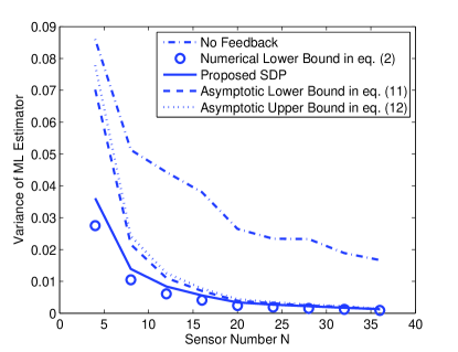
Fig. 1: Performance of the ML estimator with increasing number of sensors for $M=4$.

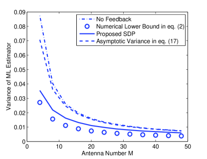
Fig. 2: Performance of the ML estimator with increasing number of antennas for $N=4$.

6 Conclusion

In this paper, we investigated a phase-only analog encoding scheme for a distributed sensor network composed of single-antenna sensors and a multi-antenna FC. We relaxed the phase optimization problem to an SDP and the numerical results show that the performance of the proposed method is close to the theoretical lower bound. Also, asymptotic results for cases with large numbers of sensors or antennas were derived. The asymptotic results indicate that when the number of senors is large and the variance of the distance between the sensor nodes and the FC is small, the availability of multiple antennas at the FC does not provide a benefit compared with the single antenna case. On the other hand, when the number of antennas $M$ is large and the measurement noise and the additive noise satisfy $M\sigma_{v,i}^{2}\ll\sigma_{n}^{2}d_{i}^{2\alpha}$, a reduction in estimation variance of $M$ can be obtained.

References

• [1] S.Β Cui, J.-J. Xiao, A.Β J. Goldsmith, Z.-Q. Luo, and H.Β V. Poor, β€œEstimation diversity and energy efficiency in distributed sensing,” IEEE Trans. Signal Process., vol. 55, no. 9, pp. 4683–4695, Sep. 2007.
• [2] M.Β K. Banavar, C.Β Tepedelenlioglu, and A.Β Spanias, β€œEstimation over fading channels with limited feedback using distributed sensing,” IEEE Trans. Signal Process., vol. 58, no. 1, pp. 414–425, Jan. 2010.
• [3] A.Β S. Leong and S.Β Dey, β€œOn scaling laws of diversity schemes in decentralized estimation,” IEEE Trans. Info. Theory, vol. 57, no. 7, pp. 4740–4759, Jul. 2011.
• [4] J.-J. Xiao, S.Β Cui, Z.-Q. Luo, and A.Β J. Goldsmith, β€œLinear coherent decentralized estimation,” IEEE Trans. Signal Process., vol. 56, no. 2, pp. 757–770, Feb. 2008.
• [5] A.Β D. Smith, M.Β K. Banavar, C.Β Tepedelenlioglu, and A.Β Spanias, β€œDistributed estimation over fading macs with multiple antennas at the fusion center,” in Proc. IEEE Asilomar 2009, Nov. 2009, pp. 424–428.
• [6] S.Β M. Kay, Fundamentals of Statistical Signal Processing: Estimation Theory, NJ: Prentice Hall, 1993.
• [7] M.Β Grant and S.Β Boyd, β€œCVX: Matlab software for disciplined convex programming, version 1.21,” http://cvxr.com/cvx, Apr. 2011.
• [8] Y.Β Zhang and A.Β M.-C. So, β€œOptimal spectrum sharing in MIMO cognitive radio networks via semidefinite programming,” IEEE J. Sel. Areas Commun., vol. 29, no. 2, pp. 362–373, Feb. 2011.