Interference-Aware Scheduling for Connectivity in MIMO Ad Hoc Multicast Networks

Abstract

We consider a multicast scenario involving an ad hoc network of co-channel MIMO nodes in which a source node attempts to share a streaming message with all nodes in the network via some pre-defined multi-hop routing tree. The message is assumed to be broken down into packets, and the transmission is conducted over multiple frames. Each frame is divided into time slots, and each link in the routing tree is assigned one time slot in which to transmit its current packet. We present an algorithm for determining the number of time slots and the scheduling of the links in these time slots in order to optimize the connectivity of the network, which we define to be the probability that all links can achieve the required throughput. In addition to time multiplexing, the MIMO nodes also employ beamforming to manage interference when links are simultaneously active, and the beamformers are designed with the maximum connectivity metric in mind. The effects of outdated channel state information (CSI) are taken into account in both the scheduling and the beamforming designs. We also derive bounds on the network connectivity and sum transmit power in order to illustrate the impact of interference on network performance. Our simulation results demonstrate that the choice of the number of time slots is critical in optimizing network performance, and illustrate the significant advantage provided by multiple antennas in improving network connectivity.

I Introduction

I-A Motivation

Interference management in co-channel ad hoc networks is a challenging problem. Simple time-division multiple access (TDMA)-based designs are inefficient and usually result in relatively poor performance. While multiple antennas are useful in enhancing channel gain and reducing interference, incorporating the extra degrees of freedom offered by MIMO (multi-input, multi-output) nodes into the design of the network further complicates matters. Designs based purely on spatial-division multiple access (SDMA) are not appropriate for large networks, since the number of available antennas is usually insufficient for cancelling all of the co-channel interference. Consequently, space-time (STDMA) solutions must generally be employed, in which multiple network links are scheduled into each time slot, and beamforming techniques are used within each slot to mitigate the resulting interference.

Prior work that has addressed STDMA scheduling for ad hoc networks has typically focused on finding solutions that maximize the sum throughput of the network [1, 2, 3, 4]. However, such solutions inevitably lead to links with poor performance and localized network congestion, which cannot be tolerated in applications where the network must perform multicast streaming [5]. An alternative is of course to use techniques that ensure fairness (i.e., max-min rate, proportional-fair scheduling, etc.) [6, 7, 8], but such techniques typically do not directly address network reliability. Performance may be fair, but how likely are the links able to achieve this performance?

The goal of this paper is to suggest methods for addressing the above issues using physical (PHY) layer techniques in combination with interference-aware scheduling. We introduce a novel definition of network connectivity that quantifies the probability that all links in the ad hoc network are able to achieve a certain pre-specified throughput. The PHY-layer parameters (beamforming vectors, transmit powers) and the scheduling decisions are then made to maximize this connectivity metric, taking into account the interference produced by links that are simultaneously active. The scenario we have in mind is ad hoc multicast network streaming, in which a source node attempts to transmit a continuous data stream to all other nodes in the ad hoc network with maximum reliability. Applications of this problem include tactical military networks (source is the unit commander, other nodes are teams or individuals under its direction), sensor surveillance networks (source is a sensor streaming data from a detected event, network nodes are monitoring stations attempting to form a coordinated response), vehicular ad hoc networks (VANETs), etc. For example, a typical VANET scenario involves a vehicle in the network that detects an unsafe road condition that must be reported to all other network nodes. In such a case, throughput is not the most important aspect of the network, since the actual message may be relatively short. Instead, the reliability of the network in sharing the message from the source with all the vehicles in the network is the key to achieving safety [9, 10]. Mobile sensing with distributed platforms (e.g., ground-based robots or UAVs) is another VANET application where connectivity is more critical than throughput, at least until a detection occurs. In sensing mode, such a network must continually be connected in order to arrive at consensus regarding the parameter(s) being sensed, or until one of them detects an object of interest, in which case the network may reconfigure itself for high-throughput data gathering.

Connectivity is fundamentally different from both throughput and energy consumption, which are the metrics most commonly used to quantify the performance of a wireless network. Connectivity performance is more relevant for applications where robustness or reliability is the most critical factor, applications (e.g., such as in military or emergency response scenarios) where the overriding concern is ensuring that information is shared with all nodes in the network at some pre-determined minimum rate. Throughput and energy consumption do not address network robustness. Instead, we argue that the connectivity of the network, as defined in the paper, is a reasonable way to measure the network’s robustness, and thus we set about choosing the network parameters to maximize the connectivity metric. A solution that achieved a higher throughput or lower energy consumption than our solution would necessarily have poorer connectivity and hence less robustness, and thus be a less desirable operating condition for the type of applications we assume.

Our focus is on how the use of multiple antennas in the network can lead to dramatic improvements in connectivity. The additional spatial degrees of freedom offered by the antennas reduce interference between the links, they allow a “denser” scheduling of users for a given set of resources, and they reduce the amount of transmit power (and hence interference to other links) to achieve a given throughput. The combined gain of these effects can only be observed by considering the joint optimization of the transmit beamformers, scheduling and power control. Unlike individuals with hand-held communication devices, VANET nodes are typically not power constrained and are large enough to support the use of multiple antennas. Thus, vehicular communication systems are a natural platform on which to consider the performance of multiple-antenna communications. Since mobility is a defining aspect of VANETs, it is important to account for the impact of the resulting time-varying wireless channels. Unlike most work in multiple-antenna ad hoc networks, we explicitly take the time-varying channels into account and quantify their impact on the reliability (connectivity) of the network.

I-B Background

This work draws on ideas and techniques that have been studied by many others, but in different contexts, including connectivity, beamforming for interference networks, and interference-based scheduling. Relevant prior work in these areas is briefly discussed below.

Investigations of radio network connectivity have been conducted by researchers over the last several decades. The original connectivity paradigm was expressed in terms of the so-called “geometric disk” model and percolation theory. In the geometric disk model, two nodes are assumed to be directly connected if their distance is smaller than some minimum transmission radius. This results in a simple binary description of connectivity (i.e., the network either is or is not connected) but lacks an indication of the quality of information flow. Percolation theory revolves around finding node density conditions under which a given node belongs to an unbounded cluster of connected nodes [11, 12]. However, neither of these approaches is reasonable for realistic networks, where one must consider the effects of fading and interference. The impact of fading on network connectivity has been addressed in [13, 14, 15, 16]. Of particular interest to this paper is [13], which showed that multiple antennas can significantly reduce the node isolation probability in an interference-free network, and [16], whose simulation results demonstrated that multiple antennas can significantly enhance the connectivity of an ad hoc network, measured as the number of links that meet a given requirement on the outage capacity, or the symbol error rate of orthogonal space-time block coding. Interference aspects of the problem have been studied in [17], which investigated the connectivity of sensor networks with regular topologies. The network connectivity was defined as the probability that a path exits between any two pairs of nodes in the network, and simulation results illustrated how an increase in node density led to decreased connectivity due to interference effects.

To reduce the impact of interference in ad hoc networks, interference graph and coloring techniques have been used in the design of scheduling or routing algorithms [18, 19, 20]. In [18], a linear programming (LP) method was proposed for computing lower and upper bounds for the maximum throughput that can be supported by a multi-hop network. A conflict (interference) graph was used to find the constraint conditions for the LP formulation. In [19], the authors proposed the construction of a link-directional interference graph to account for the directional traffic over each network link. They investigated a coloring algorithm with two colors on the interference graph to schedule transmissions in ad hoc networks employing TDMA or frequency division multiple access (FDMA). In [20], active links in a multi-hop network are scheduled in an STDMA scheme where a frame is divided into equal length time slots and each time slot can be allocated to several links simultaneously. Utilizing the interference graph, a heuristic algorithm is proposed to minimize the frame length under a constraint that each link’s minimum data rate requirement is satisfied. An earlier version of this paper [21] discusses the use of interference graphs together with MIMO for improved connectivity.

The use of multiple antennas to improve the performance of ad hoc networks has been a topic of considerable recent research [22]. For example, in [23], the transmitter for each link uses the principal singular vector of the channel matrix as the transmit beamformer and each receiver uses MMSE beamforming to mitigate the inter-link interference, and it was shown that there exists an optimal number of active links that maximize the network throughput. Beyond this value, the network becomes interference-limited, and performance is degraded. The results in [24] show if each link transmits a single data stream without CSI, while the receiver uses partial-zero-forcing interference cancellation, the capacity lower bound increases linearly with the number of antennas. In [3], an optimal scheduling policy is proposed that can maximize the average sum rate of the MIMO ad hoc network under the constraint that the average data rate of each link is larger than a certain threshold. In [7], two optimization problems are considered: one is to maximize the sum rate under sum power and proportional fairness constraints, and the other is to minimize the sum transmit power under a constraint on the minimum data rate of each link. In [1], several distributed scheduling methods were proposed for MIMO ad hoc networks. In these methods, the links whose channel condition satisfy a pre-defined threshold are divided into groups for simultaneous data transmission to maximize the overall network throughput. Also relevant is the recent research on MIMO interference networks, where techniques based on interference alignment [25] and game theory [26] have been proposed.

I-C General Approach and Contributions

As mentioned earlier, in this paper we consider PHY-layer optimization and scheduling for an ad hoc MIMO network in multicast streaming mode. In particular, we assume a source node desires to stream data to all other nodes in the network via a pre-determined multi-hop routing table (for example, a minimum spanning tree). Our emphasis will be on obtaining high reliability and low congestion for the network by maximizing the network connectivity, which we define as the probability that all links are able to support the desired throughput. The contributions of this work are as follows:

1. We examine the multi-hop multicast streaming problem using a detailed PHY-layer model, and demonstrate the significant benefit that multiple antennas, power control and proper scheduling can have on network robustness.

2. We propose a new definition of ad hoc network connectivity that approximates the probability that all links in the network can achieve a certain average throughput. The metric provides a continuous measure of connectivity performance that is more descriptive than the simple binary metrics often used in wireless networks. In addition, this metric leads to a more robust solution for fast fading channels than techniques based on requiring that only the average rate of each link be above some threshold [3, 7].

3. Since optimal connectivity will require that network links be simultaneously active, we develop beamforming and power control algorithms for the MIMO interference channels in each time slot that maximize the network connectivity metric.

4. Together with the beamforming algorithm, we propose an approach for STDMA scheduling based on greedy coloring of the interference graph that finds near-optimal assignments of links to each time slot.

5. Unlike nearly all prior work in this area, both the beamforming and scheduling algorithms take into account the fact that the channel state information (CSI) may be outdated when it is used, and we illustrate the impact of the outdated CSI on connectivity. This is particularly important for VANET applications, where the network nodes are mobile.

6. We illustrate via a number of simulations the dramatic improvement in connectivity that can be obtained when the network nodes are equipped with multiple antennas. By jointly considering the problems of beamformer design, scheduling and power control, we observe that the use of multiple antennas provides a “multiplicative” benefit” that exceeds what one would expect from their use in addressing the problems individually. Furthermore, our simulations indicate that adding antennas to the network nodes actually reduces the relative performance loss due to outdated CSI.

7. We derive analytic expressions for an upper bound on the network connectivity and a lower bound on the sum transmit power of the network assuming interference-free transmissions and no CSI errors. These optimistic bounds provide benchmarks to determine the robustness of the proposed approach.

We note here that a key limitation of the proposed approach is that the optimization described above takes place assuming that the multicast routing tree is pre-determined and remains fixed. This is clearly suboptimal since the routing decisions determine the links, which in turn create the interference environment to be mitigated. In principle, a complete cross-layer solution would jointly address the routing, scheduling and PHY-layer issues all at once, but such a problem is very complex and remains a topic of future investigation.

The rest of the paper is organized as follows. Section II describes the assumed network-level model, introduces the definition of the network connectivity metric and formulates the general optimization problem to be solved. Section III then presents the link-level MIMO model, which includes a description of the time-evolution of the MIMO channels and the outdated CSI. Section IV describes the max-connectivity beamforming solution, and Section V puts everything together in the scheduling algorithm, with an appropriate power control iteration to reduce the transmit power on each link to its minimum possible value. Performance bounds on connectivity and sum transmit power are derived in Section VI, and results from a collection of simulation studies are presented in Section VII to illustrate the performance of the algorithm. Section VIII then concludes the paper and summarizes our results. The notation used in the paper is summarized in Table I.

TABLE I: Summary of Notations

$N$	Number of nodes in the network
$M$	Number of antennas per node
$N_{L}$	Number of links in the network spanning tree
$C_{req}$	Data rate requirement for active links
$N_{s}$	Number of time slots in a frame
$SINR_{k}$	The signal-to-interference-plus-noise ratio of the $k$th link
$SINR_{t}$	Threshold for $SINR_{k}$ to guarantee the data rate requirement
$P_{out,k}$	Outage probability for the $k$th link
$U$	Network connectivity metric
$x_{k}$	Data symbol transmitted over the $k$th link
$\mathbf{t}_{k}$	Transmit beamformer for the $k$th link
$P_{k}$	Transmit power of the $k$th link
$d_{ik}$	Distance between the transmitter of link $i$ and the receiver of link $k$
$\alpha$	Path loss exponent
$\mathbf{H}_{ik}$	Channel matrix between the transmitter of link $i$ and the receiver of link $k$
$\mathbf{H}_{ik}^{e}$	Estimate of the channel between the transmitter of link $i$ and the receiver of link $k$
$\sigma_{k,1}$	Largest singular value of $\mathbf{H}_{ik}^{e}$
$\mathbf{E}_{ik}$	Channel perturbation for the link between the transmitter of link $i$ and the receiver of link $k$
$\gamma$	Channel temporal correlation coefficient
$\mathbf{n}_{k}$	Additive noise vector at receiver of link $k$
$\mathbf{w}_{k}$	Receive beamformer at receiver of link $k$
$S_{P,k}$	Scheduling priority of link $k$

II Network Model and Connectivity Definition

In this section, we provide a model for the network configuration and the physical layer channel assumed in this paper. We also define a connectivity metric for the network, which is the performance objective we wish to optimize.

II-A Network Configuration and Assumptions

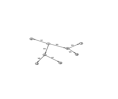
Figure 1: Transmission graph based on a multicast network with 8 nodes, where node 1 is the source node, and $v_{i}$ is a label used to denote each link.

We consider a multi-hop wireless network with a set of $N$ nodes, each of which is equipped with $M$ antennas (the assumption of an equal number of antennas is not strictly necessary, but simplifies the presentation). We assume that a source node wants to share a streaming message with all other nodes in the network through a pre-defined routing tree, as depicted for example in Figure 1. To avoid congestion and maintain a constant average data flow from the source to all nodes, each link must achieve a certain minimum data rate with high probability. Performance beyond that achievable with simple TDMA-based protocols is possible with the availability of multiple antennas, but co-channel interference must be managed through appropriate scheduling, power control and transmit/receive beamforming. The ability of the network to achieve these goals depends heavily on the accuracy of the CSI available to the scheduler, as well as that available to each link of the network.

The scheduling and transmit parameter design are centralized, and are based on outdated CSI fed back to the scheduler from the individual links. Consequently, we avoid the use of spatial multiplexing and assume that the data on each link is transmitted via a single data stream using a single transmit beamformer. The signal-to-interference-plus-noise ratio (SINR) of this data stream determines the rate of the link. Design of the receive beamformers and power control is performed by the receivers on each link, who are assumed to be aware of the statistics of the interference and the instantaneous effective CSI (channel times transmit beamformer). The source message is assumed to be broken down into packets, and the transmission is conducted over multiple frames. Each frame is divided into time slots, and each link in the routing tree is assigned one time slot in which to transmit its current packet. The scheduler determines the number of time slots and which links are active in each time slot, in order to optimize the connectivity of the network (defined below). The problem with dividing the frame into too many slots (emphasizing time rather than space-time multiplexing of the links) is that, for a fixed frame duration, the slot length is shorter, thus requiring a higher SINR to achieve the same throughput over the frame. This is the fundamental trade-off: fewer slots means more interference, but a lower SINR requirement; many slots means less interference, but a higher SINR requirement. We want to find the optimal number of slots for the best performance.

II-B Link Throughput Requirement

For a given frame, we assume that each of the active links will be allocated a single time slot, and during this time slot, each transmitter can occupy the entire available system bandwidth to send its data packet to the intended receiver. Define $C_{req}$ to be the minimum rate at which a link can be considered connected, and let the number of slots in a frame be $N_{s}$. For link $k$ to meet the rate requirement, its SINR should satisfy the following condition:

$$SINR_{k}\geq SINR_{t},$$ (1)

where $SINR_{t}=2^{N_{s}C_{req}}-1$. Due to fading and co-channel interference, the actual $SINR_{k}$ may be smaller than $SINR_{t}$. A link is said to experience an outage when the SINR at the receiver is smaller than the threshold $SINR_{t}$. The outage probability for link $k$ is thus

$$P_{out,k}=\mathrm{Pr}\{SINR_{k}<SINR_{t}\}.$$ (2)

II-C Definition of Network Connectivity

We assume that the main goal of the network is robustness rather than throughput. We want to allocate the resources of the network (transmit power, beamformers, scheduling) such that the network remains connected with the highest possible probability, where the term “connected” implies that each link is able to communicate at or above the minimum acceptable rate $C_{req}$. This in turn requires that an active link must have a certain minimum SINR. We define the connectivity as the likelihood that all the links in the network can achieve a SINR that allows transmission at or above the desired minimum data rate. Note that this is significantly different from simply requiring that the average rate be above some threshold, which is the approach taken in prior work on fast fading channels.

If the network interference has been properly managed so that its impact on a given link is negligible, then the probability of a successful transmission on a given link is independent of the other links, and the connectivity metric can be defined as

$$U=\prod_{k=1}^{N_{L}}(1-P_{out,k}).$$ (3)

According to this definition, the network connectivity is equal to the probability that none of the links in the network experiences an outage during the transmission frame. Assuming a network of $N_{L}$ links and a frame with $N_{s}$ slots, $SINR_{k}$ can be expressed as a general function of the transmission parameters:

$$SINR_{k}=f(\mathbf{t}_{1},\cdots,\mathbf{t}_{N_{L}},P_{1},\cdots,P_{N_{L}},N_{s},\mathcal{S}\;|\mathcal{H}),$$ (4)

where $\mathbf{t}_{k}\in\mathbb{C}^{M\times 1}$ and $\{\mathbf{t}_{k}|k=1,\cdots,N_{L}\}$ denotes the link beamformers, $\{P_{1},\cdots,P_{N_{L}}\}$ is the transmit power allocated to each link, $\mathbf{H}_{ik}\in\mathbb{C}^{M\times M}$ and $\mathcal{H}=\{\mathbf{H}_{ik}|i,k=1,\cdots,N_{L}\}$ represents the channels between the transmitter of link $i$ and receiver of link $k$, $\mathcal{S}=\{s_{1},\cdots,s_{N_{L}}\}$ indicates the link scheduling scheme, $s_{k}$ is the slot number allocated to link $k$, and $s_{k}\in\{1,\cdots,N_{s}\}$. Based on (4), the connectivity can thus be expressed as

$$U=\prod_{k=1}^{N_{L}}{\mathbb{E}\{I(SINR_{k})\}}=\prod_{k=1}^{N_{L}}\int{I(SINR_{k}|\mathcal{H})}p(\mathcal{H})d\mathcal{H},$$ (5)

where $p(\mathcal{H})$ denotes the probability density function (PDF) of $\mathcal{H}$ and $I(\cdot)$ is the indicator function defined as

$$I(SINR_{k})=\left\{\begin{array}[]{lr}1&\textrm{$SINR_{k}\geq SINR_{t}$}\\ 0&\textrm{$SINR_{k}<SINR_{t}$}.\end{array}\right.$$ (6)

Under this definition, when the connectivity of the network is high (near one), the total network throughput would be approximately bounded below by the number of network links times $C_{req}$. To achieve a higher total throughput, $C_{req}$ could be increased, but this would likely reduce the connectivity. A desirable trade-off between connectivity and throughput could conceivably be reached by appropriately adjusting the minimum link rate $C_{req}$.

The optimization problem associated with maximizing the connectivity of the network could thus be expressed as

$$\max\limits_{\{P_{k}\}_{k=1}^{N_{L}},\{\mathbf{t}_{k}\}_{k=1}^{N_{L}},N_{s},\mathcal{S}} U$$ (7)

$$\mathrm{subject\quad to} \|\mathbf{t}_{k}\|=1,$$

$$P_{k}\leq P_{\max}\;,\;\forall k\in\{1,\cdots,N_{L}\},$$

where $P_{\max}$ denotes an upper bound on the transmit power. Direct optimization of (7) is intractable, since one cannot find a closed-form expression for the probability of (6) in terms of the parameters of interest. Instead, we choose to solve the following related optimization problem:

$$\max\limits_{\{P_{k}\}_{k=1}^{N_{L}},\{\mathbf{t}_{k}\}_{k=1}^{N_{L}},N_{s},\mathcal{S}} \sum_{k=1}^{N_{L}}I\big{(}SINR_{k}|{\mathcal{H}}\big{)}$$ (8)

$$\mathrm{subject\quad to} \|\mathbf{t}_{k}\|=1,$$

$$P_{k}\leq P_{\max}\;,\;\forall k\in\{1,\cdots,N_{L}\}\;.$$

The relationship between this simplified problem and the original optimization is analogous to the relationship between the geometric and arithmetic means. Instead of maximizing the product of the link connection probabilities, we maximize its sum.

We divide the solution of (8) into two sub-problems: (1) scheduling and (2) beamformer design and power allocation. We solve sub-problem (2) for different results of sub-problem (1) to determine which scheduling result is best. The transmit beamforming problem is discussed in the next section, and the scheduling algorithm is described in Section V.

III Interference Channel Model with Outdated CSI

III-A Interference Channel Model

Assume without loss of generality that links $1,\cdots,N_{k}$ are simultaneously active with link $k$ during a given time slot ($k>N_{k}$). The signal at link $k$’s receiver can be expressed as

$$\mathbf{y}_{k}=\sqrt{\frac{P_{k}}{d_{kk}^{\alpha}}}\mathbf{H}_{kk}\mathbf{t}_{k}x_{k}+\sum_{i=1}^{N_{k}}\sqrt{\frac{P_{i}}{d_{ik}^{\alpha}}}\mathbf{H}_{ik}\mathbf{t}_{i}x_{i}+\mathbf{n}_{k},$$ (9)

where the transmitted symbol $x_{k}$ is a unit-magnitude data symbol, $d_{ik}$ is the distance between the transmitter of link $i$ and receiver of link $k$, $\alpha$ is the path loss exponent, and $\mathbf{n}_{k}\in\mathbb{C}^{M\times 1}$ is an additive, spatially white noise vector with covariance given by $\mathbb{E}\{\mathbf{n}_{k}\mathbf{n}_{k}^{H}\}=\sigma^{2}\mathbf{I}$ and $\mathbf{I}$ is the $M\times M$ identity matrix.

Assuming receiver $k$ employs a beamformer $\mathbf{w}_{k}\in\mathbb{C}^{M\times 1}$, the SINR for link $k$ is given by

$$SINR_{k}=\frac{\mathbb{E}\bigg{\{}\Big{|}\sqrt{\frac{P_{k}}{d_{kk}^{\alpha}}}\mathbf{w}_{k}^{H}\mathbf{H}_{kk}\mathbf{t}_{k}x_{k}\Big{|}^{2}\bigg{\}}}{\mathbb{E}\bigg{\{}\Big{|}\sum_{i=1}^{N_{k}}\sqrt{\frac{P_{i}}{d_{ik}^{\alpha}}}\mathbf{w}_{k}^{H}\mathbf{H}_{ik}\mathbf{t}_{i}x_{i}+\mathbf{w}_{k}^{H}\mathbf{n}_{k}\Big{|}^{2}\bigg{\}}}=\frac{P_{k}}{d_{kk}^{\alpha}}\frac{\big{|}\mathbf{w}_{k}^{H}\mathbf{H}_{kk}\mathbf{t}_{k}\big{|}^{2}}{\mathbf{w}_{k}^{H}\mathbf{Q}_{k}\mathbf{w}_{k}},$$ (10)

where $\mathbf{Q}_{k}=\sum_{i=1}^{N_{k}}\frac{P_{i}}{d_{ik}^{\alpha}}\mathbf{H}_{ik}\mathbf{t}_{i}(\mathbf{H}_{ik}\mathbf{t}_{i})^{H}+\sigma^{2}\mathbf{I}$. Assuming the receiver knows the covariance matrix $\mathbf{Q}_{k}$ and the channel vector $\mathbf{H}_{kk}\mathbf{t}_{k}$, the optimal $\mathbf{w}_{k}$ that maximizes $SINR_{k}$ is given by [27]:

$$\mathbf{w}_{k}=\mathbf{Q}_{k}^{-1}\mathbf{H}_{kk}\mathbf{t}_{k},$$ (11)

and the resulting SINR for link $k$ can be expressed as

$$SINR_{k}=\frac{P_{k}}{d_{kk}^{\alpha}}\mathbf{t}_{k}^{H}\mathbf{H}_{kk}^{H}\mathbf{Q}_{k}^{-1}\mathbf{H}_{kk}\mathbf{t}_{k}.$$ (12)

III-B Outdated CSI

The CSI at the scheduler will be outdated due to the time required for this information to be fed back from the network nodes. To quantify the CSI uncertainty due to the feedback delay, we adopt a first order Markov model to characterize the time variation of the channel [28]

$$\mathbf{H}_{ik}=\sqrt{1-\gamma}\mathbf{H}_{ik}^{e}+\sqrt{\gamma}\mathbf{E}_{ik},\quad i,\;k=1,\ldots,N_{L}$$ (13)

where $\mathbf{H}_{ik}$ denotes the channel matrix during the data transmission period, $\mathbf{H}_{ik}^{e}$ represents the channel feedback, and $\mathbf{E}_{ik}\in\mathbb{C}^{M\times M}$ is a perturbation matrix. The elements of $\mathbf{H}_{ik}^{e}$ and $\mathbf{E}_{ik}$ are assumed to be i.i.d complex Gaussian random variables with distribution $\mathcal{CN}(0,1)$. The coefficient $\gamma$ is used to determine the level of uncertainty in the CSI at the scheduler. In effect, under this model the scheduler assumes a Gaussian distribution for $\mathbf{H}_{ik}$, with mean $\sqrt{1-\gamma}\mathbf{H}^{e}_{ik}$ and independent entries with variance $\gamma$.

Substituting (13) into (12), the SINR at the receiver of link $k$ can be expressed as

$$SINR_{k}=\frac{P_{k}}{d_{kk}^{\alpha}}\mathbf{t}_{k}^{H}\left(\sqrt{1-\gamma}\mathbf{H}_{kk}^{e}+\sqrt{\gamma}\mathbf{E}_{kk}\right)^{H}\mathbf{Q}_{k}^{-1}\left(\sqrt{1-\gamma}\mathbf{H}_{kk}^{e}+\sqrt{\gamma}\mathbf{E}_{kk}\right)\mathbf{t}_{k},$$ (14)

where $\mathbf{Q}_{k}\!=\!\sum_{i=1}^{N_{k}}\frac{P_{i}}{d_{ik}^{\alpha}}\left(\sqrt{1-\gamma}\mathbf{H}_{ik}^{e}+\sqrt{\gamma}\mathbf{E}_{ik}\right)\mathbf{t}_{i}\mathbf{t}_{i}^{H}\left(\sqrt{1-\gamma}\mathbf{H}_{ik}^{e}+\sqrt{\gamma}\mathbf{E}_{ik}\right)^{H}+\sigma^{2}\mathbf{I}.$ It is observed that $SINR_{k}$ is a function of the channel set $\bar{\mathcal{H}}=\{\mathbf{H}_{ik}^{e}|i,k=1,\ldots,N_{L}\}$ and the channel perturbation set $\mathcal{E}\!=\!\{\mathbf{E}_{ik}|i,k\!=\!1,\ldots,N_{L}\}$. Given the channel set $\bar{\mathcal{H}}$, $SINR_{k}$ is a random variable, the distribution of which depends on the elements in $\mathcal{E}\!$. The conditional expectation of $\!SINR_{k}\!$ with respect to $\mathcal{E}\!$ is given by

$${}\mathbb{E}\{SINR_{k}|\bar{\mathcal{H}}\} = \mathbb{E}\bigg{\{}\frac{P_{k}}{d_{kk}^{\alpha}}\mathbf{t}_{k}^{H}\left(\sqrt{1-\gamma}\mathbf{H}_{kk}^{e}+\sqrt{\gamma}\mathbf{E}_{kk}\right)^{H}\mathbf{Q}_{k}^{-1}\left(\sqrt{1-\gamma}\mathbf{H}_{kk}^{e}+\sqrt{\gamma}\mathbf{E}_{kk}\right)\mathbf{t}_{k}\bigg{\}}$$

$$\overset{a}{=} \mathbb{E}\bigg{\{}\frac{P_{k}}{d_{kk}^{\alpha}}\mathbf{t}_{k}^{H}\left(\sqrt{1-\gamma}\mathbf{H}_{kk}^{e}+\sqrt{\gamma}\mathbf{E}_{kk}\right)^{H}\mathbb{E}\Big{\{}\mathbf{Q}_{k}^{-1}\Big{\}}\left(\sqrt{1-\gamma}\mathbf{H}_{kk}^{e}+\sqrt{\gamma}\mathbf{E}_{kk}\right)\mathbf{t}_{k}\bigg{\}}$$

$$= \frac{P_{k}}{d_{kk}^{\alpha}}\bigg{(}(1-\gamma)\mathbf{t}_{k}^{H}\mathbf{H}_{kk}^{eH}\mathbb{E}\Big{\{}\mathbf{Q}_{k}^{-1}\Big{\}}\mathbf{H}_{kk}^{e}\mathbf{t}_{k}+\gamma\mathrm{tr}\Big{(}\mathbb{E}\Big{\{}\mathbf{Q}_{k}^{-1}\Big{\}}\Big{)}\bigg{)},$$

where step (a) is due to the fact that perturbation matrices $\mathbf{E}_{ik}(i,k=1,\ldots,N_{L})$ are independent of each other and $\mathrm{tr}(\cdot)$ denotes the trace operator. Note that the use of the expected value in (III-B) is due to the fact that the CSI in $\mathcal{H}$ may not be precisely known. According to (13), the channel may have changed from the time it was reported since the network nodes may be mobile. If precise CSI is available, then the expectation can be dropped and the instantaneous value of $\mathcal{H}$ can be used instead. Calculation of the term $\mathbb{E}\Big{\{}\mathbf{Q}_{k}^{-1}\Big{\}}$ is very complicated, so instead we use the following lower bound based on Jensen s inequality[29, Lemma 4]:

$${}\mathbb{E}\Big{\{}\mathbf{Q}_{k}^{-1}\Big{\}} \succeq \mathbb{E}\Big{\{}\mathbf{Q}_{k}\Big{\}}^{-1}$$ (16)

$$= \mathbb{E}\left\{(1-\gamma)\sum_{i=1}^{N_{k}}\frac{P_{i}}{d_{ik}^{\alpha}}\mathbf{H}_{ik}^{e}\mathbf{t}_{i}\mathbf{t}_{i}^{H}\mathbf{H}_{ik}^{eH}+\sqrt{\gamma(1-\gamma)}\sum_{i=1}^{N_{k}}\frac{P_{i}}{d_{ik}^{\alpha}}\Big{(}\mathbf{H}_{ik}^{e}\mathbf{t}_{i}\mathbf{t}_{i}^{H}\mathbf{E}_{ik}^{H}+\mathbf{E}_{ik}\mathbf{t}_{i}\mathbf{t}_{i}^{H}\mathbf{H}_{ik}^{eH}\Big{)}\right.$$

$$\left.+\;\gamma\bigg{\{}\sum_{i=1}^{N_{k}}\frac{P_{i}}{d_{ik}^{\alpha}}\mathbf{E}_{ik}\mathbf{t}_{i}\mathbf{t}_{i}^{H}\mathbf{E}_{ik}^{H}\bigg{\}}+\sigma^{2}\mathbf{I}\right\}^{-1}$$

$$= \left((1-\gamma)\sum_{i=1}^{N_{k}}\frac{P_{i}}{d_{ik}^{\alpha}}\mathbf{H}_{ik}^{e}\mathbf{t}_{i}\mathbf{t}_{i}^{H}\mathbf{H}_{ik}^{eH}+\sqrt{\gamma(1-\gamma)}\sum_{i=1}^{N_{k}}\frac{P_{i}}{d_{ik}^{\alpha}}\mathbb{E}\left\{\mathbf{H}_{ik}^{e}\mathbf{t}_{i}\mathbf{t}_{i}^{H}\mathbf{E}_{ik}^{H}+\mathbf{E}_{ik}\mathbf{t}_{i}\mathbf{t}_{i}^{H}\mathbf{H}_{ik}^{eH}\right\}\right.$$

$$\left.+\;\gamma\sum_{i=1}^{N_{k}}\frac{P_{i}}{d_{ik}^{\alpha}}\mathbb{E}\left\{\mathbf{E}_{ik}\mathbf{t}_{i}\mathbf{t}_{i}^{H}\mathbf{E}_{ik}^{H}\right\}+\sigma^{2}\mathbf{I}\right)^{-1}$$

$$= \left(\bigg{(}\gamma\sum_{i=1}^{N_{k}}\frac{P_{i}}{d_{ik}^{\alpha}}+\sigma^{2}\bigg{)}\mathbf{I}+(1-\gamma)\sum_{i=1}^{N_{k}}\frac{P_{i}}{d_{ik}^{\alpha}}\mathbf{H}_{ik}^{e}\mathbf{t}_{i}\mathbf{t}_{i}^{H}\mathbf{H}_{ik}^{eH}\right)^{-1},$$

where $\mathbf{A}\succeq\mathbf{B}$ denotes that $\mathbf{A}-\mathbf{B}$ is a positive semidefinite matrix. In the above calculation, we use the fact that $\mathbf{E}_{ik}\mathbf{t}_{i}\in\mathbb{C}^{M\times 1}$ is a complex Gaussian random vector with distribution $\mathbf{E}_{ik}\mathbf{t}_{i}\thicksim\mathcal{CN}(0,\mathbf{I})$. Substituting (16) into (III-B), the conditional expectation of the $SINR_{k}$ is lower bounded by

$$\mathbb{E}\{SINR_{k}|\bar{\mathcal{H}}\} \geq \frac{P_{k}}{d_{kk}^{\alpha}}(1-\gamma)\mathbf{t}_{k}^{H}\mathbf{H}_{kk}^{eH}\!\!\left(\bigg{(}\gamma\sum_{i=1}^{N_{k}}\frac{P_{i}}{d_{ik}^{\alpha}}+\sigma^{2}\bigg{)}\mathbf{I}+(1-\gamma)\sum_{i=1}^{N_{k}}\frac{P_{i}}{d_{ik}^{\alpha}}\mathbf{H}_{ik}^{e}\mathbf{t}_{i}\mathbf{t}_{i}^{H}\mathbf{H}_{ik}^{eH}\right)^{\!-1}\!\!\mathbf{H}_{kk}^{e}\mathbf{t}_{k}$$ (17)

$$+\;\gamma\mathrm{tr}\left(\left(\bigg{(}\gamma\sum_{i=1}^{N_{k}}\frac{P_{i}}{d_{ik}^{\alpha}}+\sigma^{2}\bigg{)}\mathbf{I}+(1-\gamma)\sum_{i=1}^{N_{k}}\frac{P_{i}}{d_{ik}^{\alpha}}\mathbf{H}_{ik}^{e}\mathbf{t}_{i}\mathbf{t}_{i}^{H}\mathbf{H}_{ik}^{eH}\right)^{-1}\right).$$

IV Transmit Beamforming for Connectivity

In this section we introduce how the transmit beamformer and power are calculated for a given link schedule. Consider a scenario in which $K$ links are transmitting simultaneously. In this case, the number of links that can meet the desired rate requirement depends on the beamformer and transmit power that each link adopts. Define $\mathbb{E}_{l}\{SINR_{k}|\bar{\mathcal{H}}\}$ as the right hand side of (17). The problem of finding the optimal beamformer and transmit power based on the outdated CSI $\bar{\mathcal{H}}$ can be stated as:

$$\max\limits_{\{P_{k}\}_{k=1}^{K},\{\mathbf{t}_{k}\}_{k=1}^{K}} \sum_{k=1}^{K}I\big{(}\mathbb{E}_{l}\{SINR_{k}|\bar{\mathcal{H}}\}\big{)}$$ (18)

$$\mathrm{subject\;to} \|\mathbf{t}_{k}\|=1,$$

$$P_{k}\leq P_{\max}\;,\;\forall k\in\{1,\cdots,K\}.$$

The indicator function in (18) is not continuous and thus the problem is difficult to solve with standard optimization algorithms. Using the following sigmoid approximation [30]:

$$\tilde{I}\big{(}\mathbb{E}_{l}\{SINR_{k}|\bar{\mathcal{H}}\}\big{)}\approx\frac{1}{1+e^{-\beta(\mathbb{E}_{l}\{SINR_{k}|\bar{\mathcal{H}}\}-SINR_{t})}}\;,$$ (19)

where $\beta$ is the approximation parameter, the problem can be converted to finding the maximum value of a constrained continuous nonlinear multivariable function. Replacing $I\big{(}\mathbb{E}_{l}\{SINR_{k}|\bar{\mathcal{H}}\}\big{)}$ with $\tilde{I}\big{(}\mathbb{E}_{l}\{SINR_{k}|\bar{\mathcal{H}}\}\big{)}$, the optimization problem in (18) can be approximated as

$$\max\limits_{\{P_{k}\}_{k=1}^{K},\{\mathbf{t}_{k}\}_{k=1}^{K}} \sum_{k=1}^{K}\frac{1}{1+e^{-\beta(\mathbb{E}_{l}\{SINR_{k}|\bar{\mathcal{H}}\}-SINR_{t})}}$$ (20)

$$\mathrm{subject\;to} \|\mathbf{t}_{k}\|=1,$$

$$P_{k}\leq P_{\max}\;,\;\forall k\in\{1,\cdots,K\}.$$

Note that when $\beta$ is small, the sigmoid function $\tilde{I}\big{(}\mathbb{E}_{l}\{SINR_{S,k}|\bar{\mathcal{H}}\}\big{)}$ is smooth. As $\beta\rightarrow\infty$, the sigmoid function approaches the indicator function. Starting with relatively small values for $\beta$ and then increasing it in several steps, the solution involving the indicator function can be found. For each fixed value of $\beta$, the problem in (20) can be solved numerically using, for example, the active-set method. The algorithm can be initialized with arbitrary power allocations, and by setting the transmit beamformer $\mathbf{t}_{k}$ equal to the principal singular vector of $\mathbf{H}_{kk}^{e}$.

V Scheduling for Maximum Connectivity

In this section, we propose a scheduling algorithm that maximizes the connectivity metric defined earlier using the concept of coloring from graph theory[19, 20]. The algorithm is based on the use of the interference and collision graph (ICG) of the network[3, 19, 20, 18].

V-A The Interference Graph and Greedy Coloring

We use an ICG to model the relationships between the active links. In the ICG, each vertex represents a directional link in the transmission graph. We define two types of neighbors in the ICG. The first are interfering neighbors, which represent links that could be simultaneously active and hence interfere with one another, and the second are colliding neighbors, which represent links that cannot be active at the same time. In our application, colliding links include those that share the same transmitter, or those where a transmitter in one is a receiver in the other. All links that are not colliding are considered to be interfering, although the amount of interference between two given links could be low if they are far apart. In the paragraphs below, we more precisely define the ICG and concepts related to our scheduling algorithm.

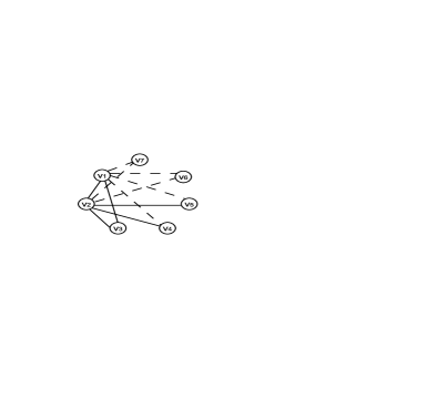
Figure 2: Partial ICG for the network of Fig. 1, where only edges corresponding to $v_{1}$ and $v_{2}$ are shown. Colliding links are connected with solid edges, interfering links with dashed edges.

Interference and collision graph: The interference and collision graph $G_{I}$ can be defined based on the transmission graph $G_{T}$. A given link $k$ in $G_{T}$ is represented by a vertex $v_{k}$ in $G_{I}$. Suppose for link $k$ that node $t_{k}$ is the transmitter and $r_{k}$ is the receiver, and suppose for link $l$ that $t_{l}$ is the transmitter and $r_{l}$ is the receiver. Links $v_{k}$ and $v_{l}$ are colliding links if any of the following are true: $t_{k}=t_{l},t_{k}=r_{l}$ or $t_{l}=r_{k}$ (note that for the multicast tree we assume, $r_{k}=r_{l}$ will never occur). An edge between two vertices in $G_{I}$ represents that the two corresponding links are colliding links and they could not be assigned to the same time slot; if two vertices in $G_{I}$ do not share an edge, they represent interfering links which can be assigned to the same time slot, provided that the resulting interference could be managed. As an illustration, Fig. 2 represents a partial ICG for the network of Fig. 1, where the colliding links and interfering links are connected with solid and dashed edges, respectively (for the sake of clarity, only edges associated with $v_{1}$ and $v_{2}$ are plotted; the remainder of the edges can be generated in a similar fashion). For example, links $v_{2}$ and $v_{1}$ share the same transmitter node 1, so they are colliding links in Fig. 2; the receiver of link $v_{2}$ is the same as the transmitter of link $v_{4}$, so $v_{2}$ and $v_{4}$ are also colliding links.

Coloring: In our application, “coloring” refers to the process of assigning time slots to the network links, or equivalently, to the nodes in the interference graph. Given a set of colors in the discrete set $\mathcal{C}$ (colors can be considered as distinct non-negative integers), a coloring of the graph $G$ is an assignment of the elements (or colors) in $\mathcal{C}$ to the vertices of $G$, one color for each vertex, such that no adjacent vertices occupy the same color. A greedy coloring enumerates the vertices in a specific order $v_{1},\dots,v_{n}$ and assigns $v_{k}$ to the smallest color that is not occupied by the neighbors of $v_{k}$ among $v_{1},\dots,v_{k-1}$. The vertices can be ordered according to their edge degree, which is the number of edges incident to the vertex [31, chap. 5]. To apply coloring to the ICG, we need to define an order for the vertices. Before we proceed to the scheduling order, some related definitions are necessary.

Scheduling freedom: For a link $k$, the scheduling freedom $F_{k}$ is the number of available colors that can be allocated to this link. The higher the value of $F_{k}$, the higher the possibility that link $k$ will be allocated to a “good” color (one that leads to low interference).

Collision degree: Given a link $k$, the collision degree $C_{D,k}$ is the number of its colliding neighbors in the ICG.

Constraint and free color sets: For link $k$, the interfering color set $\mathcal{D}_{I,k}$ includes colors occupied by the neighbors that interfere with $v_{k}$. The unavailable color set $\mathcal{D}_{U,k}$ includes the colors occupied by the neighbors that collide with $v_{k}$. The free color set is defined as $\mathcal{D}_{F,k}=\mathcal{C}-(\mathcal{D}_{I,k}\bigcup\mathcal{D}_{U,k})$, and corresponds to the set of colors that could be assigned to link $k$ without causing any interference (or collisions). The constraint color set is defined as $\mathcal{D}_{C,k}=\mathcal{D}_{I,k}-(\mathcal{D}_{I,k}\bigcap\mathcal{D}_{U,k})$. The colors in this set can also possibly be assigned to link $k$, but with some additional interference that would have to be mitigated through beamforming.

Scheduling priority: The scheduling order is determined using the largest singular values $\sigma_{k,1}$ of the channel matrices $\mathbf{H}_{kk}^{e}$. The higher the value of $C_{D,k}$ or the smaller the channel gain $g_{k}=\sigma_{k,1}^{2}/d_{kk}^{\alpha}$, the more likely it is that link $k$ will be affected by interference. Such a link will have fewer colors it could be assigned to, and hence a smaller value of $F_{k}$. To increase the likelihood that links with low scheduling freedom can be allocated a good color, the scheduling priority of link $k$ is defined as

$$S_{P,k}=C_{D,k}\cdot W+\frac{1}{g_{k}},$$ (21)

where $W$ is a constant larger than $\max_{k}\frac{1}{g_{k}}$.

V-B Scheduling Algorithm for Connectivity

Based on the above definitions, we propose here a scheduling algorithm for optimizing connectivity. The algorithm assumes a particular value for the number of slots $N_{s}$, and is repeated until a value of $N_{s}$ is found that maximizes the connectivity metric. The minimum possible value for $N_{s}$ is the maximum collision degree $\max_{k}C_{D,k}$ over all vertices in the ICG. The algorithm begins by ordering the links according to their scheduling priority, and then assigns a color to them one-by-one, from highest to lowest priority. Consider the link at position $m$ in the priority ordering. If link $m$ can be added to a color that already has had other links assigned to it, and if the beamformers and power levels for these links can be adjusted to accommodate link $m$ without causing any of them to drop below $SINR_{t}$, then link $m$ is added to this color. If there are multiple colors for which this is true, it is added to the color that requires the smallest increase in transmit power to accommodate it. If the addition of link $m$ to any of these colors causes one of the links (including possibly link $m$) to drop below the SINR threshold, and if there exist free colors that have not had any links assigned to them, link $m$ is assigned to one of the free colors. If no free colors exist, then link $m$ is assigned to the color that caused the smallest number of links to drop below the threshold (and with the smallest increase in power, in case of a tie). In this latter case, it is hoped that the power control algorithm described in the next section will reduce the interference sufficiently so that all links assigned to the color will end up being active. A more precise mathematical description of the algorithm is given below.

1. Let $\mathbf{v}_{k}$ be the right singular vector of $\mathbf{H}_{kk}^{e}$ corresponding to the largest singular value, and let $P_{k}=P_{\max}$ be the initial transmit power allocated to link $k$. Assuming a value for $N_{s}$, initialize the active link set $\mathcal{A}=\{k\;|\;P_{\max}g_{k}\geq SINR_{t},k=1,\dots,N_{L}\}$. Links that do not qualify for $\mathcal{A}$ cannot meet the desired target rate for the given value of $N_{s}$. Initialize the transmit beamformers as $\mathcal{T}=\{\mathbf{v}_{k}|k\in\mathcal{A}\}$, the transmit powers as $\mathcal{P}=\{P_{k}=P_{\max}|k\in\mathcal{A}\}$ and the color set $\mathcal{C}=\{1,2,\cdots,N_{s}\}$. Let $\mathcal{P}_{C}=\{P_{C,1},\dots,P_{C,N_{s}}\}$ denote the sum transmit power of the active links in each color, and let $\mathcal{N}_{C}=\{N_{C,1},\dots,N_{C,N_{s}}\}$ represent the number of links that are unable to meet the the target $SINR_{t}$ for each color. Initialize these sets to contain all zeros. The initial schedule $\mathcal{S}=\{s_{k}|k\in\mathcal{A}\}$ is also set to zeros. Construct the ICG based on the relationship between the active links. Compute the scheduling priority $S_{P,k}$ of the vertices $v_{k}$ for $k\in\mathcal{A}$ .

2. Select the link with the highest scheduling priority: $m=\arg\max_{k\in\mathcal{A}}S_{P,k}$, and construct the free color set $\mathcal{D}_{F,m}$ and the constraint color set $\mathcal{D}_{C,m}$ for link $m$.

   • If $\mathcal{D}_{C,m}=\phi$ and $D_{F,m}\neq\phi$

     Assign link $m$ to color $j=\min_{i\in\mathcal{D}_{F,m}}i$, set $s_{m}=j$, $P_{m}=P_{C,j}=\frac{SINR_{t}}{g_{m}}$, and

     skip to step 5.

   • else if $\mathcal{D}_{C,m}=\phi$ and $D_{F,m}=\phi$

     There aren’t enough colors to avoid collisions between the active links, so the

     algorithm must be restarted with a larger value for $N_{s}$.

   • else

     For $i\in\mathcal{D}_{C,m}$, construct the link set $\mathcal{L}_{m,i}=\{k\;|\;s_{k}=i\;\mbox{\rm for}\;k\in\mathcal{A}\}$, which

     contains the links currently assigned to color $i$.

   • end.

3. For each $i\in\mathcal{D}_{C,m}$, assume the links in the set $\mathcal{L}_{m,i}\bigcup m$ are transmitting simultaneously, and use the transmit beamforming algorithm of Section IV to find the new beamformer and transmit power sets $\mathcal{T}_{m,i}=\{\mathbf{t}_{m,k}^{i}|k\in\mathcal{L}_{m,i}\bigcup m\}$, $\mathcal{P}_{m,i}=\{P_{m,k}^{i}|k\in\mathcal{L}_{m,i}\bigcup m\}$. For link set $\mathcal{L}_{m,i}\bigcup m$, based on $\mathcal{T}_{m,i}$, $\mathcal{P}_{m,i}$, calculate the expected number of links that will be unable to meet the SINR threshold with link $m$ added: $\tilde{N}_{m,i}=\sum_{k\in\mathcal{L}_{m,i}\bigcup m}{\Big{(}1-I\big{(}\mathbb{E}_{l}\{SINR_{k}|\bar{\mathcal{H}}\}\big{)}\Big{)}}$, and calculate the updated sum transmit power due to the addition of link $m$: $\tilde{P}_{m,i}=\sum_{k\in\mathcal{L}_{m,i}\bigcup m}P_{m,k}^{i}$. Set $\Delta N_{m,i}=\tilde{N}_{m,i}-N_{C,i}$ to be the number of links that will drop below the SINR threshold if link $m$ is added to color $i$, and define $\Delta P_{m,i}=\tilde{P}_{m,i}-P_{C,i}$ to be the additional transmit power required to add link $m$ to color $i$.

4. Find $j^{{}^{\prime}}=\arg\min_{i\in\mathcal{D}_{C,m}}{\Delta N_{m,i}}$. If more than one color corresponds to the minimum $\Delta N_{m,i}$, select the color with minimum $\Delta P_{m,i}$.

   • If $\mathcal{D}_{F,m}=\phi$ or $\Delta N_{m,j^{\prime}}=0$

     Assign link $m$ to color $j^{{}^{\prime}}$, set $s_{m}=j^{{}^{\prime}}$, $N_{C,j^{{}^{\prime}}}=\tilde{N}_{m,j^{{}^{\prime}}}$, $P_{C,j^{{}^{\prime}}}=\tilde{P}_{m,j^{{}^{\prime}}}$. Use $\mathcal{T}_{m,j^{{}^{\prime}}}$,

     $\mathcal{P}_{m,j^{{}^{\prime}}}$ to update the components of $\mathcal{T}$ and $\mathcal{P}$ which correspond to links in the set

     $\mathcal{L}_{m,j^{{}^{\prime}}}\bigcup m$.

   • else if $\mathcal{D}_{F,m}\neq\phi$ and $\Delta N_{m,j}>0$

     Assign link $m$ to color $j=\min_{i\in\mathcal{D}_{F,m}}i$ and set $s_{m}=j$, $P_{m}=P_{C,j}=\frac{SINR_{t}}{g_{m}}$.

   • end.

5. Set $S_{P,m}=0$, and repeat step 2 until each vertex $v_{k}$, $k\in\mathcal{A}$, is allocated a color.

Once the scheduling is complete, the active links will transmit data according to the scheduling result $\mathcal{S}$ using the beamformers in $\mathcal{T}$ and, at least initially, the transmit powers in $\mathcal{P}$. As explained below, the actual transmit power for each link will be fine-tuned based on feedback from the receivers.

V-C Local Power Control for Active Links

Since the nodes are energy limited, to extend the lifetime of the network and to reduce the mutual interference caused by the co-channel links, the transmit power of each link should be minimized under the constraint of the QoS requirement. Due to the approximation in (19), the use of the lower bound in (17), and the presence of outdated CSI, the actual $SINR_{k}$ based on $\mathcal{P}$ and $\mathcal{T}$ will not be exactly equal to the threshold $SINR_{t}$. In most instances it will be greater than $SINR_{t}$ due to the use of the lower bound in (17), but in some rare cases it can be below the threshold. To remedy this latter situation, we reduce the transmit power of any links whose SINR exceeds the threshold, which reduces co-channel interference and the transmit power consumed by the network. For a given time slot $t\in\mathcal{C}$, the network schedule $\mathcal{S}$ assigns links in set $\mathcal{L}_{t}=\{k|s_{k}=t,k\in\mathcal{A}\}$ to transmit simultaneously. The power control algorithm steps through each link in the time slot, reducing power for the link if its SINR exceeds the threshold. A given link may be revisited several times, since reductions in transmit power for other links reduces the overall interference, and may allow further reductions in transmit power for the link. This process is assumed to repeat a maximum of $N_{a}$ times. If, after all $N_{a}$ iterations, there are any links whose SINR is below the threshold, these links are declared to be in outage, their power is reduced to zero, and an additional $N_{b}$ iterations are performed to reduce the transmit power even further. A mathematical description of the power control algorithm for time slot $t$ is described below.

Iterative Power Control Algorithm

1. Initialize the transmit power and beamformer of link $k\in\mathcal{L}_{t}$ with $\mathcal{P}$ and $\mathcal{T}$, set maximum iteration lengths $N_{a}$ and $N_{b}$.

2. Link $k$’s receiver $(k\in\mathcal{L}_{t})$ calculates $SINR_{k}$ based on (12). If $SINR_{k}>SINR_{t}$, the receiver for link $k$ informs the transmitter to reduce $P_{k}$ to $P_{k}=\frac{P_{k}}{SINR_{k}/SINR_{t}}$.

3. $N_{a}=N_{a}-1$, if $N_{a}>0$, go to step 2.

4. If $SINR_{k}<SINR_{t}$ for any $k\in\mathcal{L}_{t}$, set $P_{k}=0$ and repeat step 2 for another $N_{b}$ iterations to further reduce the transmit power.

VI Performance Bounds

In this section, we derive two performance bounds that can be used to evaluate the limiting behavior of the proposed algorithms. The first is an upper bound on the network connectivity metric, and the second is a lower bound on the average sum transmit power. Both bounds are derived under the assumption that the CSI is perfect, and each active link is free of interference. When $\gamma$ is small, the connectivity bound should match the performance of the proposed approach if the network interference has been properly accounted for. This is not the case for the bound on transmit power, however, since the interference mitigation results in beamformers that require excess power to achieve the rate threshold. The difference between the required transmit power and the lower bound represents the price paid for the enhanced connectivity that results from operating the system as an interference network. Due to the complexity of calculating the bounds, expressions are derived only for the cases $M=1,2,4$.

VI-A Upper Bound on Network Connectivity

The connectivity bound is derived assuming the absence of interference, and perfect CSI at the scheduler ($\gamma=0$). Each transmitter uses maximum power and selects the principal singular vector of the channel matrix as its beamformer. When the receiver is free of co-channel interference, the resulting signal-to-noise-ratio (SNR) for link $k$ is given by

$$SNR_{k}=\frac{P_{\max}\sigma_{k,1}^{2}}{d_{kk}^{\alpha}\sigma^{2}}.$$ (22)

If we define $P_{out,k}^{{}^{\prime}}=\Pr\{SNR_{k}<SINR_{t}\}$, then the upper bound on connectivity can be expressed as

$$U_{B}^{M}=\prod_{k=1}^{N_{L}}(1-P_{out,k}^{{}^{\prime}})\geq U.$$ (23)

The squared singular value $\sigma_{k,1}^{2}$ corresponds to the largest eigenvalue of the central Wishart matrix $\mathbf{H}_{kk}\mathbf{H}_{kk}^{H}$. Define $\lambda_{k,1}=\sigma_{k,1}^{2}$, and note that the cumulative density function (CDF) of $\lambda_{k,1}$ is given by [32, eq. (6)]:

$$\Pr\{\lambda_{1}\leq\lambda\}=\frac{\det(\mathbf{\Phi}(\lambda))}{\left(\prod_{j=1}^{M}{\Gamma^{2}(j)}\right)},$$ (24)

where we have dropped the subscript $k$ since the distribution is assumed to be identical for each link, $\Gamma(\cdot)$ is the gamma function, $\mathbf{\Phi}(\lambda)$ is an $M\times M$ matrix defined by $\mathbf{\Phi}(\lambda)_{i,j}=\tilde{\gamma}(i+j-1,\lambda)$, and the lower incomplete gamma function $\tilde{\gamma}(n,x)$ has the following series expansion:

$$\tilde{\gamma}(n,\lambda)=(n-1)!\left(1-\sum_{k=0}^{n-1}\frac{\lambda^{k}}{k!}e^{-\lambda}\right).$$ (25)

For $M=2$, (24) reduces to:

$$\Pr\{\lambda_{1}\leq\lambda\} = \frac{\det(\mathbf{\Phi}(\lambda)_{2\times 2})}{\prod_{j=1}^{2}{\Gamma^{2}(j)}}$$ (26)

$$= \frac{\tilde{\gamma}(1,\lambda)\tilde{\gamma}(3,\lambda)-\tilde{\gamma}^{2}(2,\lambda)}{\Gamma^{2}(1)\Gamma^{2}(2)}$$

$$= 1-e^{-\lambda}(\lambda^{2}+2)+e^{-2\lambda}.$$

Substituting (26) into (23), the connectivity upper bound can then be calculated as:

$$U_{B}^{M=2}=e^{-\sum_{k=1}^{N_{L}}\lambda_{\min,k}}\prod_{k=1}^{N_{L}}\left(\lambda_{\min,k}^{2}-e^{-\lambda_{\min,k}}+2\right)\;,$$ (27)

where $\lambda_{\min,k}=\frac{SINR_{t}d_{kk}^{\alpha}\sigma^{2}}{P_{\max}}$ is the minimum value of the channel gain that can guarantee $SNR_{k}\geq SINR_{t}$.

For $M=4$, after some cumbersome algebra, the CDF of the largest eigenvalue $\lambda_{1}$ can be expressed as:

$$\Pr\{\lambda_{1}\leq\lambda\} = \frac{\det(\mathbf{\Phi}(\lambda)_{4\times 4})}{\prod_{j=1}^{4}{\Gamma^{2}(j)}}$$ (28)

$$= 1-f_{1}(\lambda)-f_{2}(\lambda)-f_{3}(\lambda)-f_{4}(\lambda),$$

where $f_{1}(\lambda)$, $f_{2}(\lambda)$, $f_{3}(\lambda)$, $f_{4}(\lambda)$ are defined in the appendix. The network connectivity upper bound is then computed as

$$U_{B}^{M=4} = \prod_{k=1}^{N_{L}}\Big{(}f_{1}(\lambda_{\min,k})+f_{2}(\lambda_{\min,k})+f_{3}(\lambda_{\min,k})+f_{4}(\lambda_{\min,k})\Big{)}.$$ (29)

For the single antenna case ($M=1$), the interference-free $SNR$ at the receiver is given by

$$SNR_{k}=\frac{P_{\max}|h_{kk}|^{2}}{d_{kk}^{\alpha}\sigma^{2}},$$ (30)

where $|h_{kk}|$ is a Rayleigh random variable. Define $h=|h_{kk}|$, so that $\Pr\{h\leq\lambda\}=1-e^{-\lambda^{2}}$. The probability of a successful transmission for the link can be expressed as

$$\Pr\{SNR_{k}\geq SINR_{t}\} = 1-\Pr\Bigg{\{}h<\sqrt{\lambda_{\min,k}}\Bigg{\}}=e^{-\lambda_{\min,k}},$$ (31)

and thus the network connectivity is given by

$$U_{B}^{M=1}=e^{-\sum_{k=1}^{N_{L}}\lambda_{\min,k}}.$$ (32)

Comparing (27) and (29) with (32), it can be observed that

$$R_{2}=\frac{U_{B}^{M=2}}{U_{B}^{M=1}} = \prod_{k=1}^{N_{L}}\left(\lambda_{\min,k}^{2}-e^{-\lambda_{\min,k}}+2\right),$$ (33)

$$R_{4}=\frac{U_{B}^{M=4}}{U_{B}^{M=1}} = \prod_{k=1}^{N_{L}}e^{\lambda_{\min,k}}\Big{(}f_{1}(\lambda_{\min,k})+f_{2}(\lambda_{\min,k})+f_{3}(\lambda_{\min,k})+f_{4}(\lambda_{\min,k})\Big{)}.$$ (34)

It is easy to verify that both $R_{2}$ and $R_{4}$ are monotonically increasing functions of $\lambda_{\min,k}$ and larger than 1. $R_{2}$ and $R_{4}$ represent the connectivity gain provided by the use of multiple antennas. Since $\lambda_{\min,k}$ is proportional to $d_{kk}^{\alpha}$, the larger the link distance, the greater the connectivity gain offered by the use of multiple antennas.

VI-B Lower Bound on Average Sum Transmit Power

A lower bound for the average sum transmit power of the network can be obtained under the assumption that each active link selects its beamformer as the right singular vector of the channel with largest singular value, and assuming there is no co-channel interference between the links.

For link $k$, given $\lambda_{1}$, the power allocation at the transmitter is:

$$P_{k}^{M}=\left\{\begin{array}[]{ll}\frac{SINR_{t}d_{kk}^{\alpha}\sigma^{2}}{\lambda_{1}},&\textrm{$\lambda_{1}\geq\lambda_{\min,k}$}\\ 0,&\textrm{$\lambda_{1}<\lambda_{\min,k}$}\end{array}\right.$$ (35)

The average transmit power of link $k$ can be obtained by averaging $P_{k}^{M}$ over the random variable $\lambda_{1}$. Denote the probability density function (PDF) of $\lambda_{1}$ as $f_{\lambda_{1}}(\lambda)$, then $f_{\lambda_{1}}(\lambda)$ can be explicitly obtained by taking the derivative of (26) or (28) with respect to $\lambda$.

When $M=2$, $f_{\lambda_{1}}^{M=2}(\lambda)$ is given by

$$f_{\lambda_{1}}^{M=2}(\lambda)=e^{-\lambda}(\lambda^{2}+2)-2\lambda e^{-\lambda}-2e^{-2\lambda}.$$ (36)

The average transmit power for link $k$ is calculated as

$$\mathbb{E}\{P_{k}^{M=2}\} = \int_{\lambda_{\min,k}}^{\lambda_{\max}}\frac{SINR_{t}d_{kk}^{\alpha}\sigma^{2}}{\lambda}f_{\lambda_{1}}^{M=2}(\lambda)d\lambda$$ (37)

$$= SINR_{t}d_{kk}^{\alpha}\sigma^{2}\int_{\lambda_{\min,k}}^{\lambda_{\max}}\lambda e^{-\lambda}-2e^{-\lambda}+\frac{2}{\lambda}\big{(}e^{-\lambda}-e^{-2\lambda}\big{)}d\lambda\;.$$

In (37), the integration of the first two terms can easily be found. To calculate the term $\int\frac{e^{-c\lambda}}{\lambda}d\lambda$ for constant $c$, we expand the exponential function $f(\lambda)=e^{-c\lambda}$ using a Taylor series. The Taylor series at the point $\hat{\lambda}$ is

$$\tilde{t}(\lambda)=\sum_{n=0}^{\infty}\frac{(-c)^{n}e^{-c\hat{\lambda}}}{n!}(\lambda-\hat{\lambda})^{n}.$$ (38)

With the help of (38), the term $\int\frac{e^{-c\lambda}}{\lambda}d\lambda$ in (37) can be further expressed as

$$g_{1}(c,\lambda) = \int\frac{e^{-c\lambda}}{\lambda}d\lambda=\int\frac{\tilde{t}(\lambda)}{\lambda}d\lambda$$ (39)

$$= \int\sum_{n=0}^{\infty}\frac{(-c)^{n}e^{-c\hat{\lambda}}}{n!}\sum_{k=0}^{n}\binom{n}{k}(-\hat{\lambda})^{(n-k)}\lambda^{k-1}d\lambda$$

$$= \int\frac{e^{-c\hat{\lambda}}}{\lambda}+\sum_{n=1}^{\infty}\frac{(-c)^{n}e^{-c\hat{\lambda}}}{n!}\left(\frac{(-\hat{\lambda})^{n}}{\lambda}+\sum_{k=1}^{n}\binom{n}{k}(-\hat{\lambda})^{(n-k)}\lambda^{k-1}\right)d\lambda$$

$$= e^{-c\hat{\lambda}}\ln\lambda+\sum_{n=1}^{\infty}\frac{(-c)^{n}e^{-c\hat{\lambda}}}{n!}\left((-\hat{\lambda})^{n}\ln\lambda+\sum_{k=1}^{n}\binom{n}{k}(-\hat{\lambda})^{(n-k)}\frac{\lambda^{k}}{k}\right),$$

and the average transmit power for link $k$ can be written using the following expression:

$$\mathbb{E}\{P_{k}^{M=2}\} = SINR_{t}d_{kk}^{\alpha}\sigma^{2}\big{(}(1-\lambda_{\max})e^{-\lambda_{\max}}-(1-\lambda_{\min,k})e^{-\lambda_{\min,k}}+2g_{1}(1,\lambda_{\max})$$ (40)

$$-2g_{1}(1,\lambda_{\min,k})-g_{1}(2,\lambda_{\max})+g_{1}(2,\lambda_{\min,k})\big{)}.$$

Similarly, when $M=4$, the PDF of $\lambda_{1}$ can be expressed as:

$${}f_{\lambda_{1}}^{M=4}(\lambda)=f_{1}^{{}^{\prime}}(\lambda)+f_{2}^{{}^{\prime}}(\lambda)+f_{3}^{{}^{\prime}}(\lambda)+f_{4}^{{}^{\prime}}(\lambda),$$ (41)

where the definitions of $f_{1}^{{}^{\prime}}(\lambda)$, $f_{1}^{{}^{\prime}}(\lambda)$, $f_{1}^{{}^{\prime}}(\lambda)$, $f_{1}^{{}^{\prime}}(\lambda)$ can be found in the appendix. The average transmit power for link $k$ in this case is given by

$$\mathbb{E}\{P_{k}^{M=4}\} = \int_{\lambda_{\min,k}}^{\lambda_{\max}}\frac{SINR_{t}d_{kk}^{\alpha}\sigma^{2}}{\lambda}f_{\lambda_{1}}^{M=4}(\lambda)d\lambda$$ (42)

$$= SINR_{t}d_{kk}^{\alpha}\sigma^{2}\int_{\lambda_{\min,k}}^{\lambda_{\max}}\frac{1}{\lambda}\Big{(}f_{1}^{{}^{\prime}}(\lambda)+f_{2}^{{}^{\prime}}(\lambda)+f_{3}^{{}^{\prime}}(\lambda)+f_{4}^{{}^{\prime}}(\lambda)\Big{)}d\lambda\;.{}$$

Based on (VIII)-(50) in the appendix, the average transmit power in (42) can be evaluated as

$$\mathbb{E}\{P_{k}^{M=4}\} = SINR_{t}d_{kk}^{\alpha}\sigma^{2}\Big{(}\hat{f}_{1}(\lambda_{\max})-\hat{f}_{1}(\lambda_{\min,k})+\hat{f}_{2}(\lambda_{\max})-\hat{f}_{2}(\lambda_{\min,k})+\hat{f}_{3}(\lambda_{\max})$$ (43)

$$-\hat{f}_{3}(\lambda_{\min,k})+\hat{f}_{4}(\lambda_{\max})-\hat{f}_{4}(\lambda_{\min,k})\Big{)}.$$

For the single-antenna case, we average the transmit power over the channel gain $h_{kk}$ to determine the average transmit power of link $k$ as

$$\mathbb{E}\{P_{k}^{M=1}\} = \int_{\sqrt{\lambda_{\min,k}}}^{\lambda_{\max}}\frac{2SINR_{t}d_{kk}^{\alpha}\sigma^{2}}{h}e^{-h^{2}}dh$$ (44)

$$= 2SINR_{t}d_{kk}^{\alpha}\sigma^{2}\Big{(}\tilde{s}(\lambda_{\max})-\tilde{s}\big{(}\sqrt{\lambda_{\min,k}}\big{)}\Big{)},$$

where the function $\tilde{s}(x)$ is defined as

$$\tilde{s}(x)=\int\frac{e^{-x^{2}}}{x}dx=\ln{x}+\sum_{n=1}^{\infty}(-1)^{n}\frac{x^{2n}}{2n\cdot n!}.$$ (45)

Thus, the lower bound on the average sum transmit power of the $N_{L}$ links is given by

$$P_{B}^{M}=\frac{1}{N_{s}}\sum_{k=1}^{N_{L}}\mathbb{E}\{P_{k}^{M}\}.$$ (46)

VII Simulation Results

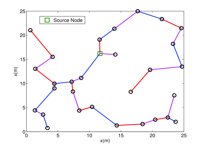
Figure 3: The topology of the network assumed for the simulation with $N=30$ nodes.

For our simulations, we consider a network with $N=30$ nodes, uniformly distributed in a $25\textrm{m}\times 25\textrm{m}$ area as shown in Fig. 3. The node represented by a square is the source node, and the edges represent the $N_{L}=29$ links in the multicast tree. Also in Fig. 3, the scheduling result for a single channel realization is provided when $N_{s}=3$, $M=4$, $\gamma=0.04$ and $C_{req}=0.9\textrm{bps/Hz}$; the links that have the same color have been scheduled to transmit in the same time slot. We assume noise with unit power, a maximum transmit power of $P_{\max}=25\textrm{dB}$ for each node, and a path loss exponent of $\alpha=2$. The connectivity performance and the sum transmit power of the network are averaged over 300 independent channel realizations and the performance for different $M$, $N_{s}$ and $\gamma$ is provided. Note that although the highest collision degree for any of the nodes is 4, the minimum number of slots considered for a given frame is 3, which means our scheduling algorithm can use only 3 time slots to completely avoid the link collisions.

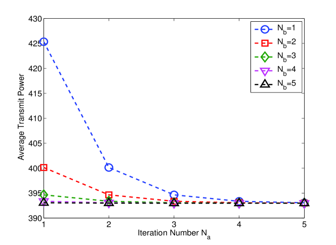
Figure 4: Average sum transmit power comparison between different $N_{a}$ and $N_{b}$, with $C_{req}=0.9\text{bps/Hz}$, $\gamma=0.01$, $N_{s}=5$ for $M=4$.

In the power control algorithm, only the first few iterations play an important role in the algorithm performance. This is illustrated in the example of Fig. 4 for a case with $M=4$, $C_{req}=0.9$ bps/Hz, $\gamma=0.1$ and $N_{s}=5$. We see that all of the power reduction occurs for $\{N_{a},N_{b}\}\leq 3$. In the simulation results that follow, we set $N_{a}=3$ and $N_{b}=2$. The minimum rate requirement $C_{req}$ in the following simulations is assumed to be adjusted to take into account the overhead due to channel estimation and feedback to the source. The QoS requirements are set to be $C_{req}=0.9\text{bps/Hz}$ for $M=4$, $C_{req}=0.5\text{bps/Hz}$ for $M=2$ and $C_{req}=0.1\text{bps/Hz}$ for $M=1$, and plots for both $\gamma=0.01$ and $\gamma=0.04$ are included. We show results for different $C_{req}$ with each $M$, due to the strong impact of the number of antennas on performance. When the connectivity probability is near 1, the approximate total throughput of the network can be found by multiplying $C_{req}$ by $N_{L}-1$ and the connectivity probability.

We compare the performance of three cases: outdated CSI (OCSI), local perfect CSI (LPCSI) and global perfect CSI (GPCSI). For OCSI, the source node uses the outdated global CSI $\bar{\mathcal{H}}$ as the input to the scheduling algorithm, and the links transmit according to the scheduling results $\mathcal{S}$, $\mathcal{T}$ and $\mathcal{P}$ provided by the source. In LPCSI, the CSI of the links transmitting in the same time slot are assumed to be known by the other active links and, based on this local CSI, the transmit beamforming algorithm is used to re-optimize the beamformers for that time slot. The performance gain of LPCSI over OCSI represents the advantage provided by the use of local instantaneous CSI. For GPCSI, we assume the source node has perfect knowledge of $\mathcal{H}$, which amounts to assuming $\gamma=0$. For this case, the lower bound on SINR in (18) is replaced with the exact SINR expression in (12). The results for GPCSI indicate the best performance that the scheduling algorithm can achieve, and we see that as predicted, its performance matches the bound in Section VI-A, provided that $N_{s}$ is chosen large enough so that the interference can be properly mitigated.

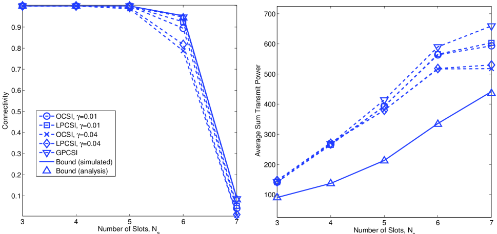
Figure 5: Connectivity performance and average sum transmit power of the network for different number of time slots per frame, with $M=4$, $C_{req}=0.9\text{bps/Hz}$.

Fig. 5 provides the connectivity performance and the average sum transmit power for $M=4$. The behavior of the connectivity metric can be explained as follows. As the number of colors (slots) increases, the number of links that transmit simultaneously will be reduced, the interference between the links will thus be reduced, and the SINR at the receiver of each link will be improved. However, to guarantee the spectral efficiency $C_{req}$, the threshold $SINR_{t}$ must also increase due to the shorter time slot. When the benefit brought by the increase in the number of slots is larger than the penalty caused by the increased $SINR_{t}$, the connectivity of the network will increase; otherwise, the connectivity will decrease. This trade-off results in an optimal value for $N_{s}$ for each case considered.

The behavior of the transmit power curves is slightly different, since links that cannot meet the desired SINR are not allowed to transmit. This obviously reduces the connectivity metric, but it also reduces the total transmit power. That explains why, for example, the transmit power required by GPCSI is always higher than that for the other cases; since it achieves a higher connectivity, more links are active and more transmit power is consumed. Note also that the analytical values for both the connectivity and transmit power bounds match those obtained in the simulation. It can be observed that when $\gamma=0.04$, full connectivity is achieved at $C_{req}=0.9\text{bps/Hz}$ with a required transmit power of about 150. Comparing the performance of GPCSI and OCSI for $\gamma=0.04$, we see no impact of the outdated CSI on the network connectivity for $N_{s}\leq 5$.

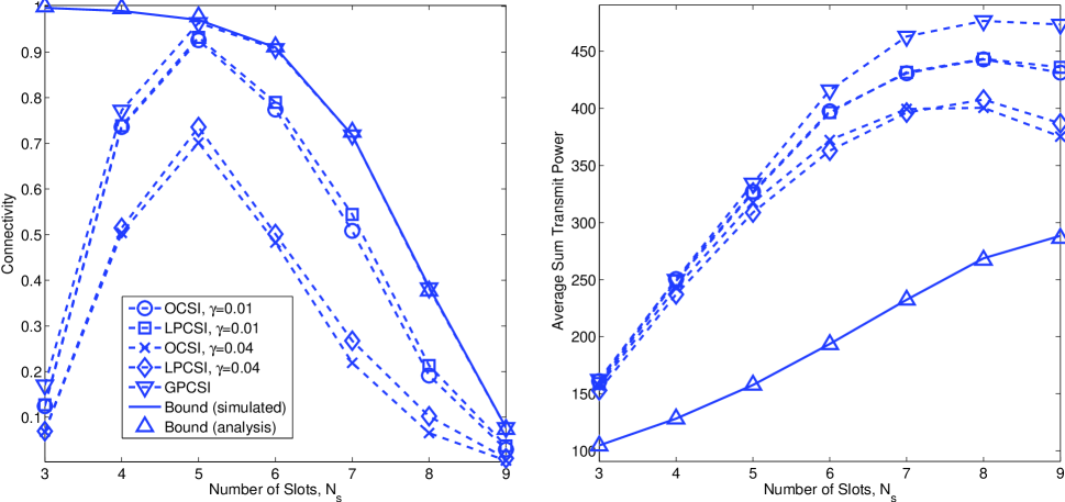
Figure 6: Connectivity performance and average sum transmit power of the network for different number of time slots per frame, with $M=2$, $C_{req}=0.5\text{bps/Hz}$.

In Fig. 6, we see that the two-antenna network is able to achieve a connectivity of about 0.7 at $C_{req}=0.5\text{bps/Hz}$, requiring a transmit power of approximately 300. Compared with GPCSI for $\gamma=0.04$ and $N_{s}=5$, the network connectivity of OCSI is reduced by about 25%.

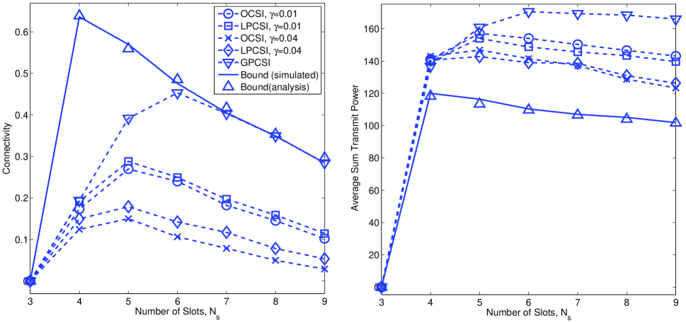
Figure 7: Connectivity performance and average sum transmit power of the network for different number of time slots per frame, with $M=1$, $C_{req}=0.1\text{bps/Hz}$.

Fig. 7 presents the performance results for $M=1$ with $C_{req}=0.1\text{bps/Hz}$. Peak connectivity occurs at $N_{s}=5$, with a required transmit power of about 140, and a connectivity of only about 0.15 is achieved. When $\gamma=0.04$, we see that the connectivity performance of OCSI is reduced by a factor of three with respect to GPCSI.

Comparing the connectivity performance in Figs. 5-7, it can be observed that the optimal value for $N_{s}$ decreases with $M$, even though we have increased the desired throughput with $M$ as well. The benefit of having nodes equipped with multiple antennas is clearly evident in terms of connectivity and total network throughput. Note that the benefit of nodes with multiple antennas also manifests itself in terms of the transmit power required to achieve maximum connectivity. Instead of a throughput gain of four with the same level of reliability, which might be expected when comparing the $M=4$ and $M=1$ networks, we see that there is a multiplicative benefit that results from using multiple antennas for improved connectivity. The additional spatial degrees of freedom reduce interference between links within the same time slot, they reduce the total number of required time slots, and they reduce the amount of transmit power (and hence interference to other links) to achieve a given throughput. The combined gain of these effects can only be observed by considering the joint optimization of the transmit beamformers, scheduling and power control.

Further evidence of the multiplicative benefit of multiple antennas is the fact that we observe a decrease in sensitivity to imprecise CSI as the number of antennas at each node increases. Note also that using locally accurate CSI to adjust the transmit beamformers (LPCSI) has only a slight benefit in improving performance relative to using the beamformers based on outdated CSI (OCSI). This is due to the fact that only a single data stream is transmitted on each link. If multiple data streams were allowed, the importance of locally accurate CSI would be more critical; one could potentially improve connectivity, but the performance gain would be much more sensitive to imprecise CSI.

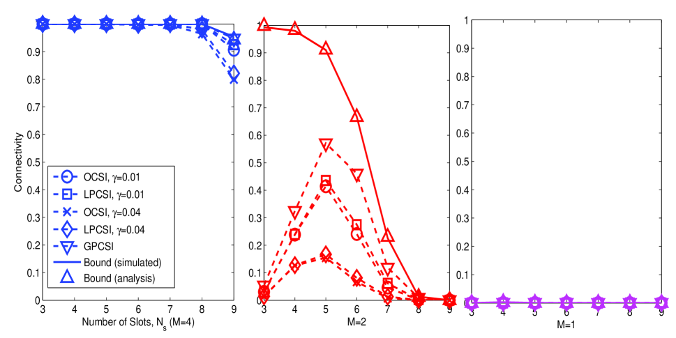
Figure 8: Connectivity comparison between different antenna configurations $M=4$, $M=2$, $M=1$, with $C_{req}=0.6\text{bps/Hz}$, $\gamma=0.01$ or $\gamma=0.04$.

In Fig. 8, we show the connectivity results for all three antenna sizes for the same value of $C_{req}=0.6$bps/Hz. The $M=4$ network achieves full connectivity in this case, while the $M=1$ network is nearly disconnected. The two-antenna case falls somewhere in between, with performance depending on how accurate the CSI is at the scheduler.

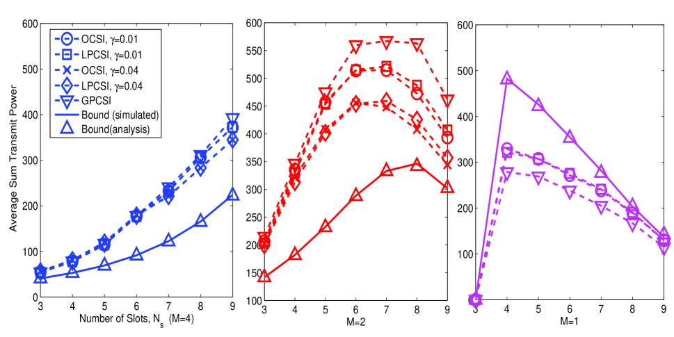
Figure 9: Average sum transmit power comparison between different antenna configurations $M=4$, $M=2$, $M=1$, with $C_{req}=0.6\text{bps/Hz}$, $\gamma=0.01$ or $\gamma=0.04$.

In Fig. 9, the transmit power results are provided. The difference in transmit power is especially evident in this example. The $M=4$ network requires a factor of seven times less power to achieve a connectivity that is five times higher than the $M=2$ case. While the single-antenna network is almost disconnected, the fact that the average sum transmit power is non-zero indicates that at least some of the links are active.

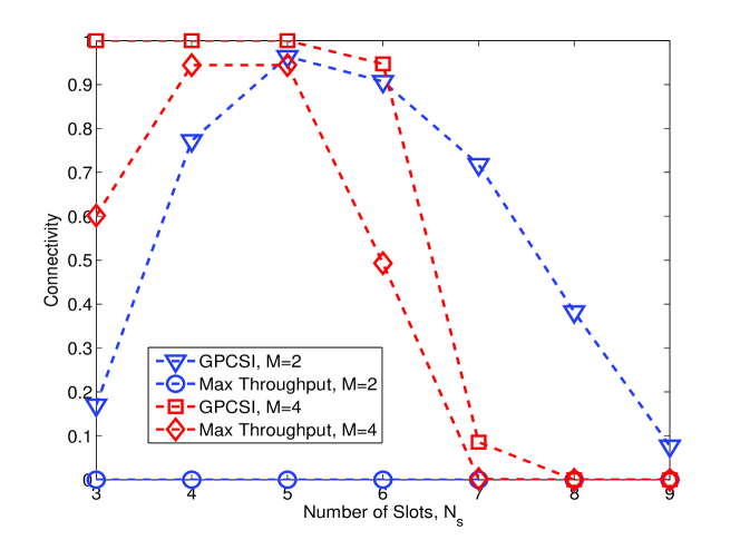
Figure 10: Connectivity performance of the network for different scheduling methods, with $C_{req}=0.5\text{bps/Hz}$ for $M=2$ and $C_{req}=0.9\text{bps/Hz}$ for $M=4$.

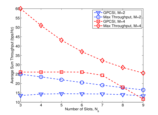
Figure 11: Average sum throughput comparison between different scheduling methods, with $C_{req}=0.5\text{bps/Hz}$ for $M=2$ and $C_{req}=0.9\text{bps/Hz}$ for $M=4$.

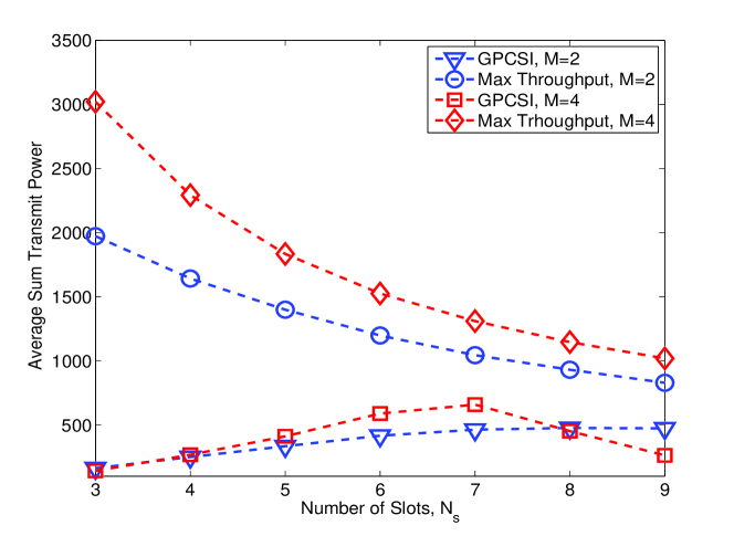
Figure 12: Average sum transmit power comparison between different scheduling methods, with $C_{req}=0.5\text{bps/Hz}$ for $M=2$ and $C_{req}=0.9\text{bps/Hz}$ for $M=4$.

Finally, in Figs. 10-12, we compare the performance of our connectivity-based approach with one that attempts to choose the network parameters in order to maximize the throughput of the network. The optimization algorithm in this case is similar to the scheduling algorithm for connectivity, with the exception that the objective function in (8) is replaced with $\sum_{k=1}^{N_{L}}\log_{2}(1+SINR_{k})$. In Fig. 10, for $M=2$, we see that attempting to maximize the throughput results in zero connectivity for the network, while using our approach, we achieve a connectivity in excess of 0.95 for the optimal value of $N_{s}=5$.

In Fig. 11, the overall network throughput of the max-throughput approach is about 50% higher than the connectivity optimization method. This indicates that a subset of the nodes is able to communicate at a higher rate, but the network is disconnected and the message from the source is not reaching all of the network nodes.

In Fig. 12, the results show that the proposed approach achieves the maximum connectivity with about five times less transmit power than the max-throughput approach. The connectivity of the max-throughput approach improves when $M=4$, but with an increase in required power consumption of nearly a factor of eight.

VIII Conclusions

In this paper we investigated the use and benefit of multiple antennas in an ad hoc network with a source streaming data to all nodes via a multi-hop tree. Based on a novel definition of network connectivity, a scheduling algorithm was developed that takes advantage of the interference mitigation capabilities of the MIMO nodes. A key component of the algorithm is the design of transmit beamformers for simultaneously active nodes that optimizes the connectivity metric. Ultimately, the scheduling algorithm acts to break down the full network into a set of smaller interference networks whose links are able to be simultaneously active due to the interference mitigation provided by the multiple antennas. We also derived performance bounds on the network connectivity and average required sum transmit power, assuming zero interference and perfect CSI. These bounds represent ultimate limits for the performance of the network, and were used in the simulations to compare against the actual behavior of the network. Our simulation results indicate the significant advantage provided by multiple antennas in the ad hoc network, in terms of connectivity, throughput, reduced transmit power and resilience to outdated CSI. By considering the joint problem of transmit beamformer design, scheduling and power control, we observe a multiplicative benefit to the use of multiple antennas for improving network reliability. Such an observation could not be made by solving each of these problems in isolation from the others.

The functions $f_{1}(\lambda)$, $f_{2}(\lambda)$, $f_{3}(\lambda)$, $f_{4}(\lambda)$ in (28) are defined as follows:

$$f_{1}(\lambda) = (e^{-\lambda}+e^{-3\lambda})\left(6\lambda^{2}+\frac{11}{6}\lambda^{4}+\frac{1}{36}\lambda^{6}\right),$$

$$f_{2}(\lambda) = (e^{-\lambda}-e^{-3\lambda})\left(-4\lambda^{3}-\frac{1}{3}\lambda^{5}\right),$$

$$f_{3}(\lambda) = -e^{-2\lambda}\left(12\lambda^{2}+\frac{2}{3}\lambda^{4}+\frac{2}{9}\lambda^{6}+\frac{1}{144}\lambda^{8}\right),$$

$$f_{4}(\lambda) = 4e^{-\lambda}+4e^{-3\lambda}-6e^{-2\lambda}-e^{-4\lambda}.$$

Based on $\!f_{1}(\lambda)$, $\!f_{2}(\lambda)$, $\!f_{3}(\lambda)$, $\!f_{4}(\lambda)$, the functions $\!f_{1}^{{}^{\prime}}(\lambda)$, $\!f_{2}^{{}^{\prime}}(\lambda)$, $\!f_{3}^{{}^{\prime}}(\lambda)$, $\!f_{4}^{{}^{\prime}}(\lambda)$ in (41) are defined as:

$$f_{1}^{{}^{\prime}}(\lambda) = -\frac{df_{1}(\lambda)}{d\lambda}=(e^{-\lambda}+e^{-3\lambda})\left(-12\lambda-\frac{22}{3}\lambda^{3}-\frac{1}{6}\lambda^{5}\right)-(e^{-\lambda}+3e^{-3\lambda})\left(-6\lambda^{2}-\frac{11}{6}\lambda^{4}-\frac{1}{36}\lambda^{6}\right),$$

$$f_{2}^{{}^{\prime}}(\lambda) = -\frac{df_{2}(\lambda)}{d\lambda}=(-e^{-\lambda}+3e^{-3\lambda})\left(4\lambda^{3}+\frac{1}{3}\lambda^{5}\right)+(e^{-\lambda}-e^{-3\lambda})\left(12\lambda^{2}+\frac{5}{3}\lambda^{4}\right),$$

$$f_{3}^{{}^{\prime}}(\lambda) = -\frac{df_{3}(\lambda)}{d\lambda}=e^{-2\lambda}\left(24\lambda+\frac{8}{3}\lambda^{3}+\frac{4}{3}\lambda^{5}+\frac{1}{18}\lambda^{7}\right)-2e^{-2\lambda}\left(12\lambda^{2}+\frac{2}{3}\lambda^{4}+\frac{2}{9}\lambda^{6}+\frac{1}{144}\lambda^{8}\right),$$

$$f_{4}^{{}^{\prime}}(\lambda) = -\frac{df_{4}(\lambda)}{d\lambda}=4e^{-\lambda}+12e^{-3\lambda}-12e^{-2\lambda}-4e^{-4\lambda}.$$

Define $g_{2}(c,n,x)=\int x^{n}e^{cx}dx=\sum_{i=0}^{n}\frac{n!}{c^{i+1}(n-i)!}x^{n-i}e^{cx}$, then it can be shown that

$${}\hskip 23.00006pt\hat{f}_{1}(\lambda)= \int\frac{f_{1}^{{}^{\prime}}(\lambda)}{\lambda}d\lambda$$

$$= -12\Big{(}g_{2}(-1,0,\lambda)\!+\!g_{2}(-3,0,\lambda)\Big{)}\!-\!\frac{22}{3}\Big{(}g_{2}(-1,2,\lambda)\!+\!g_{2}(-3,2,\lambda)\Big{)}$$

$$-\!\frac{1}{6}\Big{(}g_{2}(-1,4,\lambda)\!+\!g_{2}(-3,4,\lambda)\Big{)}+6\Big{(}g_{2}(-1,1,\lambda)\!+\!3g_{2}(-3,1,\lambda)\Big{)}$$

$$+\frac{11}{6}\Big{(}g_{2}(-1,3,\lambda)+3g_{2}(-3,3,\lambda)\Big{)}+\frac{1}{36}\Big{(}g_{2}(-1,5,\lambda)+3g_{2}(-3,5,\lambda)\Big{)},$$ (47)

$${}\hskip-95.00014pt\hat{f}_{2}(\lambda)= \int\frac{f_{2}^{{}^{\prime}}(\lambda)}{\lambda}d\lambda$$

$$= 4\Big{(}3g_{2}(-3,2,\lambda)\!-\!g_{2}(-1,2,\lambda)\Big{)}\!+\!\frac{1}{3}\Big{(}3g_{2}(-3,4,\lambda)\!-\!g_{2}(-1,4,\lambda)\Big{)}$$

$$+\!12\Big{(}g_{2}(-1,1,\lambda)\!-\!g_{2}(-3,1,\lambda)\Big{)}+\!\frac{5}{3}\Big{(}g_{2}(-1,3,\lambda)\!-\!g_{2}(-3,3,\lambda)\Big{)},$$ (48)

$${}\hskip-75.0001pt\hat{f}_{3}(\lambda)= \int\frac{f_{3}^{{}^{\prime}}(\lambda)}{\lambda}d\lambda$$

$$= 24g_{2}(-2,0,\lambda)+\frac{8}{3}g_{2}(-2,2,\lambda)+\frac{4}{3}g_{2}(-2,4,\lambda)+\frac{1}{18}g_{2}(-2,6,\lambda)$$

$$-24g_{2}(-2,1,\lambda)-\frac{4}{3}g_{2}(-2,3,\lambda)-\frac{4}{9}g_{2}(-2,5,\lambda)-\frac{1}{72}g_{2}(-2,7,\lambda),$$ (49)

$${}\hskip-40.00006pt\hat{f}_{4}(\lambda)=\int\frac{f_{4}^{{}^{\prime}}(\lambda)}{\lambda}d\lambda=4\big{(}g_{1}(1,\lambda)-g_{1}(4,\lambda)\big{)}+12\big{(}g_{1}(3,\lambda)-g_{1}(2,\lambda)\big{)}.$$ (50)

References

- [1] M. Pun, W. Ge, D. Zheng, J. Zhang, and V. Poor, “Distributed opportunistic scheduling for MIMO ad-hoc networks,” in Proc. IEEE ICC 2008, May 2008, pp. 3689–3693.
- [2] Y. Ma, R. Schober, and S. Pasupathy, “Weighted sum-rate maximization scheduling for MIMO ad hoc networks,” in Proc. IEEE ICC 2009, Jun. 2009, pp. 1–5.
- [3] J. Zheng and M. Ma, “QoS-aware cooperative medium access control for MIMO ad-hoc networks,” IEEE Commun. Letters, vol. 14, no. 1, pp. 48–50, Jan. 2010.
- [4] T. ElBatt, “Towards scheduling MIMO links in interference-limited wireless ad hoc networks,” in Proc. IEEE MILCOM 2007, Oct. 2007, pp. 1–7.
- [5] C. Cordeiro, H. Gossain, and D. Agrawal, “Multicast over wireless mobile ad hoc networks: Present and future directions,” IEEE Network, vol. 17, no. 1, pp. 52–59, Jan. 2003.
- [6] O. Somarriba and J. Zander, “Evaluation of heuristic strategies for scheduling, and power allocation in STDMA wireless networks,” in Proc. IEEE ISSSE 2007, Jul. 2007, pp. 427–430.
- [7] R. Yue and Y. Hua, “Space-time power scheduling of MIMO links - Fairness and QoS considerations,” IEEE J. Sel. Areas Commun., vol. 2, no. 2, pp. 171–180, Apr. 2008.
- [8] G. Marfia, P. Lutterotti, S. J. Eidenbenz, G. Pau, and M. Gerla, “Faircast: Fair multi-media streaming in ad hoc networks through local congestion control,” in Proc. ACM MSWiM 2008, Oct. 2008, pp. 1–9.
- [9] A. Boukerche, “Vehicular ad hoc networks: An emerging technology toward safe and efficient transportation,” in Algorithms and Protocols for Wireless, Mobile Ad Hoc Networks. Wiley-IEEE Press, 2009, pp. 405–432.
- [10] S. C. Ng, W. Zhang, Y. Zhang, Y. Yang, and G. Mao, “Analysis of access and connectivity probabilities in vehicular relay networks,” IEEE J. Sel. Areas Commun., vol. 29, no. 1, pp. 140–150, Jan. 2011.
- [11] L. Booth, J. Bruck, M. Franschetti, and R. Meester, “Covering algorithms, continuum percolation and the geometry of wireless networks,” Ann. Appl. Prob., vol. 13, no. 2, pp. 722–741, 2002.
- [12] S. Quintanilla, S. Torquato, and R. Ziff, “Efficient measurements of the percolation threshold for the fully penetrable disks,” J. Phys. A: Math. Gen., vol. 33, no. 42, pp. L399–L407, Oct. 2000.
- [13] D. Miorandi, E. Altman, and G. Alfano, “The impact of channel randomness on coverage and connectivity of ad hoc and sensor networks,” IEEE Trans. Wireless Commun., vol. 7, no. 3, pp. 1062–1072, Mar. 2008.
- [14] A. S. Ibrahim, K. G. Seddik, and K. J. R. Liu, “Connectivity-aware network maintenance and repair via relays deployment,” IEEE Trans. Wireless Commun., vol. 8, no. 1, pp. 356–366, Jan. 2009.
- [15] Z. Han, A. L. Swindlehurst, and K. J. R. Liu, “Optimization of MANET connectivity via smart deployment/movement of unmanned air vehicles,” IEEE Trans. Veh. Technol., vol. 58, no. 7, pp. 3533–3546, Sep. 2009.
- [16] H. Yousefi’zadeh, H. Jafarkhani, and J. Kazemitabar, “A study of connectivity in MIMO fading ad-hoc networks,” IEEE/KICS Journal of Communication and Networks, vol. 11, no. 1, pp. 47–56, Feb. 2009.
- [17] R. Rajagopalan and P. K. Varshney, “Connectivity analysis of wireless sensor networks with regular topologies in the presence of channel fading,” IEEE Trans. Wireless Commun., vol. 8, no. 7, pp. 3475–3483, Jul. 2009.
- [18] K. Jain, J. Padhye, V. Padmanabhan, and L. Qiu, “Impact of interference on multi-hop wireless network performance,” ACM/Springer Wireless Networks, vol. 11, no. 4, pp. 471–487, Jul. 2005.
- [19] P. C. Ng, D. J. Edwards, and S. C. Liew, “Coloring link-directional interference graphs in wireless ad hoc networks,” in Proc. IEEE Globecom 2007, Nov. 2007, pp. 859–863.
- [20] A. Behzad and I. Rubin, “Optimum integrated link scheduling and power control for multihop wireless networks,” IEEE Trans. Veh. Technol, vol. 56, no. 1, pp. 194–205, Jan. 2007.
- [21] F. Jiang, J. Wang, and A. L. Swindlehurst, “Scheduling for MIMO networks with rate-constrained connectivity requirements,” in Proc. VTC 2010 Spring, May 2010, pp. 1–5.
- [22] M. Zorzi, J. Zeidler, A. L. Swindlehurst, M. Jensen, and S. Krishnamurthy, “Cross-layer issues in MAC protocol design for MIMO ad hoc networks,” IEEE Wireless Commun., vol. 13, no. 4, pp. 62–76, Aug. 2006.
- [23] J. Ma, Y. Zhang, X. Su, and Y. Yan, “On capacity of wireless ad hoc networks with MIMO MMSE receivers,” IEEE Trans. Wireless Commun., vol. 7, no. 12, pp. 5493–5503, Dec. 2008.
- [24] R. Vaze and J. R. W. Heath, “Transmission capacity of ad-hoc networks with multiple antennas using transmit stream adaptation and interference cancelation,” submitted to the IEEE Trans. on Info. Theory, Dec. 2009.
- [25] T. Gou and S. A. Jafar, “Degrees of freedom of the K-user MxN MIMO interference channel,” IEEE Trans. Info. Theory, vol. 56, no. 12, pp. 6040–6057, Dec. 2010.
- [26] M. Nokleby and A. L. Swindlehurst, “Bargaining and multi-user detection in MIMO interference networks,” in Proc. ICCCN, Aug. 2008, pp. 509–514.
- [27] J. H. Winters, “Optimum combining in digital mobile radio with cochannel interference,” IEEE Trans. Veh. Technol., vol. 33, no. 3, pp. 144–155, Aug. 1984.
- [28] Z. Zhou, B. Vucetic, Z. Chen, and Y. Li, “Design of adaptive modulation in MIMO systems using outdated CSI,” in Proc. IEEE PIMRC 2005, Sep. 2005, pp. 1101–1105.
- [29] X. Zhang, D. P. Palomar, and B. Ottersten, “Statistically robust design for linear MIMO transceivers,” IEEE Trans. Signal Process., vol. 56, no. 8, pp. 3678–3689, Aug. 2008.
- [30] J. Wang, D. J. Love, and M. D. Zoltowski, “Minimizing the number of dropped users in MIMO multicasting channels,” in Proc. IEEE Milcom 2007, Nov. 2007, pp. 1–5.
- [31] R. Diestel, Graph Theory, 3rd ed. Springer-Verlag, 2005.
- [32] M. Kang and M.-S. Alouini, “A comparative study on the performance of MIMO MRC system with and without cochannel interference,” IEEE Trans. Commun., vol. 52, no. 4, pp. 1417–1425, Aug. 2004.