A Three Higgs Doublet Model for the Fermion Mass Hierarchy Problem

Abstract

In this paper we propose an explanation to the Fermion mass hierarchy problem by fitting the type-II seesaw mechanism into the Higgs doublet sector, such that their vacuum expectation values are hierarchal. We extend the Standard Model with two extra Higgs doublets as well as a spontaneously broken $U_{X}(1)$ gauge symmetry. All fermion Yukawa couplings except that of top quark are of ${\cal O}(10^{-2})$ in our model. Constraints on the parameter space from Electroweak precision measurements are studied. Besides, the neutral component of the new fields, which are introduced to cancel the anomalies of the $U(1)_{X}$ gauge symmetry can be dark matter candidate. We investigate its signature in the dark matter direct detection.

I Introduction

In the Standard Model (SM) of particle interactions, charged fermions get masses through the spontaneously broken of the electroweak symmetry and the Higgs mechanism, while neutrinos are massless. At $M_{Z}$, the charged lepton masses and the current masses of quarks are given by pdg

$$m_{e}\sim 0.51~{}{\rm MeV}\;\hskip 28.45274pt m_{\mu}\sim 0.105~{}~{}{\rm GeV}\;\hskip 28.45274ptm_{\tau}\sim 1.7~{}~{}{\rm GeV}$$

$$m_{u}\sim 1~{}~{}~{}~{}{\rm MeV}\;\hskip 28.45274pt m_{c}\sim 1.3~{}~{}~{}~{}~{}{\rm GeV}\;\hskip 28.45274ptm_{t}\sim 174~{}~{}{\rm GeV}$$

$$m_{d}\sim 5~{}~{}~{}~{}{\rm MeV}\;\hskip 28.45274pt m_{s}\sim 0.13~{}~{}~{}{\rm GeV}\;\hskip 28.45274ptm_{b}\sim 4~{}~{}~{}~{}~{}{\rm GeV}\;,$$

which shows an enormous hierarchy among the Yukawa couplings $y_{\psi}$. For example, we have $y_{u}/y_{t}\sim 10^{-5}$ for the quark sector.

For the neutrino sector, recent results from solar, atmosphere, accelerator and reactor neutrino oscillation experiments show that neutrinos have small but non-zero masses at the sub-eV scale and different lepton flavors are mixed. If neutrinos are Dirac particles, their masses may come from the Higgs mechanism, then we have $y_{\nu}/y_{t}\sim 10^{-12}$, which seems even unnatural. For the case neutrinos being Majorana particles, the most popular way to explain neutrino masses are the seesaw mechanismseesawI ; seesawII ; seesawIII . If we assume the Yukawa couplings between left-handed lepton doublet and right-handed neutrinos are of order $1$, then we have $m_{t}/m_{N}\sim 10^{-12}$, which is also unnatural.

In this paper, we attempt to solve or explain the charged fermion and neutrino mass hierarchy problem in the three Higgs doublet model. There are already many excellent literatures focusing on this issueFN ; etradim ; tjli ; xing ; yanagida ; nir ; ftheory ; so10 ; add ; davidson ; ding ; frogratt ; Feruglio . In our model, one Higgs doublet get its vacuum expectation value (VEV) in the same way as that of the SM Higgs boson, while the other two Higgs fields get their VEVs through the mechanism similar to type-II seesaw model, i.e., they get their VEVs through their mixings with the SM Higgs. Such that the VEVs can be normal hierarchal, which is guaranteed by the spontaneously broken $U(1)$ gauge symmetry. We set them to be $v_{1}=100~{}MeV$, $v_{2}=10~{}GeV$ and $v_{3}=173~{}GeV$ in our paper. For each generation of charged fermions, there is one Higgs field responsible the origin of their masses. For the neutrino sector, there are only Yukawa couplings with the first generation Higgs field. Such that Dirac neutrino mass matrix is naturally small without requiring small Yukawa coupling constants. Then active neutrinos may get small but non-zero masses through the TeV-scale seesaw mechanism ernestma . We introduce some new fields to cancel anomalies of the $U(1)_{X}$ gauge symmetry, and the neutral component of them can be cold dark matter candidate. We will study its signatures in dark matter direct detection experiments.

The note is organized as follows: In section II we give a brief introduction to the model, including particle contents, Higgs potential and scalar mass spectrum. Section III is devoted to study the fermion masses. We investigate constraints on the model from Electroweak precision measurements and dark matter phenomenology in section IV and V. The last part is concluding and remarks.

II The model

Fields	$q^{u}_{L}$	$q_{L}^{c}$	$q_{L}^{t}$	$u_{R}$	$c_{R}$	$t_{R}$	$d_{R}$	$s_{R}$	$b_{R}$	$\ell_{L}$	$e_{R}$	$\mu_{R}$	$\tau_{R}$	$\nu_{R}^{i}$	$\psi_{L}^{i}$	$\eta_{L}^{k}$	$\xi_{L}^{k}$	$\eta_{R}^{k}$	$\xi_{R}^{k}$	$H_{1}$	$H_{2}$	$H_{3}$	$\Phi$
$U_{X}(1)$	1	-1	0	2	-2	0	0	0	0	0	-1	1	0	1	1	1	-1	0	0	1	-1	0	1

Table 1: Particle contents and their quantum numbers under $U_{X}(1)$ gauge symmetry. $i=1,2,3$ and $k=1,\cdots 6$. $q_{L}^{u}=(u_{L},d_{L})^{T}$,$q_{L}^{c}=(c_{L},s_{L})^{T}$, $q_{L}^{t}=(t_{L},b_{L})^{T}$, $\ell_{L}$ denotes left-handed lepton doublets.

We extend the SM with three right-handed neutrinos, two extra Higgs doublet, one Higgs singlet as well as a flavor dependent $U(1)_{X}$ gauge symmetry. Six generation fermion singlets $\eta$($\xi$) with $U(1)_{X}$ hypecharge $(-)1$ as well as three generation fermion singlets $\psi_{L}$ with $U(1)_{X}$ hypecharge $0$ are introduced to cancel the anomalies. The particle contents and their representation under the $U(1)$ gauge symmetry are listed in table 1. We apply the type-II seesaw mechanism to the Higgs doublet sector. The most general Higgs potential can be written as

$${\cal L}_{\rm Higgs} = +m_{1}^{2}H_{1}^{\dagger}H_{1}+m_{2}^{2}H_{2}^{\dagger}H_{2}-m_{3}^{2}H_{3}^{\dagger}H_{3}-m_{0}^{2}\Phi^{\dagger}\Phi+\lambda_{0}(\Phi^{\dagger}\Phi)^{2}+\lambda_{1}(H_{1}^{\dagger}H_{1})^{2}+\lambda_{2}(H_{2}^{\dagger}H_{2})^{2}$$ (2)

$$+\lambda_{3}(H_{3}^{\dagger}H_{3})^{2}+\lambda_{4}(H_{1}^{\dagger}H_{1})(H_{2}^{\dagger}H_{2})+\lambda_{5}(H_{1}^{\dagger}H_{1})(H_{3}^{\dagger}H_{3})+\lambda_{6}(H_{2}^{\dagger}H_{2})(H_{3}^{\dagger}H_{3})$$

$$+\lambda_{7}(H_{1}^{\dagger}H_{2})(H_{2}^{\dagger}H_{1})+\lambda_{8}(H_{1}^{\dagger}H_{3})(H_{3}^{\dagger}H_{1})+\lambda_{9}(H_{2}^{\dagger}H_{3})(H_{3}^{\dagger}H_{2})+\lambda_{10}(\Phi^{\dagger}\Phi)(H_{1}^{\dagger}H_{1})$$

$$+\lambda_{11}(\Phi^{\dagger}\Phi)H_{2}^{\dagger}H_{2}+\lambda_{12}\Phi^{\dagger}\Phi H_{3}^{\dagger}H_{3}$$

$$+\left(\lambda_{13}(H_{3}^{\dagger}H_{1})(H_{3}^{\dagger}H_{2})+\mu_{1}\Phi H_{3}^{\dagger}H_{1}+\mu_{2}\Phi^{\dagger}H_{3}^{\dagger}H_{2}+{\rm h.c.}\right)\;.$$

It is obviously that $H_{1}$ and $H_{2}$ shall develop no VEVs without terms in the bracket of Eq. 2. The conditions for ${\cal L}_{\rm Higgs}$ develops minimum involve four constraint equations. By assuming $\langle H\rangle=v_{1}/\sqrt{2}$, $\langle\eta\rangle=v_{2}/\sqrt{2}$, $\langle\varphi\rangle=v_{3}/\sqrt{2}$ and $\langle\Phi\rangle=v_{4}/\sqrt{2}$, we have

$$+m_{1}^{2}v_{1}+\lambda_{1}v_{1}^{3}+{1\over 2}v_{1}\left[(\lambda_{4}+\lambda_{7})v_{2}^{2}+(\lambda_{5}+\lambda_{8})v_{3}^{2}+\lambda_{10}v_{4}^{2}\right]+{1\over 2}\lambda_{13}v_{2}v_{3}^{2}+\mu_{1}v_{3}v_{4}=0\;,$$

$$+m_{2}^{2}v_{2}+\lambda_{2}v_{2}^{3}+{1\over 2}v_{2}\left[(\lambda_{4}+\lambda_{7})v_{1}^{2}+(\lambda_{6}+\lambda_{9})v_{3}^{2}+\lambda_{11}v_{4}^{2}\right]+{1\over 2}\lambda_{13}v_{2}v_{3}^{2}+\mu_{2}v_{3}v_{4}=0\;,$$

$$-m_{3}^{2}v_{3}+\lambda_{3}v_{3}^{3}+{1\over 2}v_{3}\left[(\lambda_{5}+\lambda_{8})v_{1}^{2}+(\lambda_{6}+\lambda_{9})v_{2}^{2}+\lambda_{12}v_{4}^{2}\right]+{\lambda_{13}}v_{1}v_{2}v_{3}+\mu_{1}v_{1}v_{4}+\mu_{2}v_{2}v_{4}=0\;,$$

$$-m_{0}^{2}v_{4}+\lambda_{0}v_{4}^{3}+{1\over 2}v_{4}\left[\lambda_{10}v_{1}^{2}+\lambda_{11}v_{2}^{2}+\lambda_{12}v_{3}^{2}\right]+\mu_{1}v_{1}v_{3}+\mu_{2}v_{2}v_{3}=0\;.$$ (3)

Let $m_{i}^{2},\lambda_{i}>0$, $\lambda_{13}=0$(for simplificity) and $|\mu_{i}|\ll m_{i}$, then we have

$$v_{1}\approx{\mu_{1}v_{3}v_{4}\over m_{1}^{2}}\;,\hskip 14.22636ptv_{2}\approx{\mu_{2}v_{3}v_{4}\over m_{2}^{2}}\;,\hskip 14.22636ptv_{3}^{2}\approx{m_{3}^{2}\over\lambda_{3}}\;,\hskip 14.22636ptv_{4}^{2}\approx{m_{0}^{2}\over\lambda_{0}}\;.$$ (4)

Notice that $v_{1}$ and $v_{2}$ are suppressed by their masses, which is quite similar to that in the type-II seesaw mechanism. So we can get relatively small $v_{1}$ and $v_{2}$ without conflicting with any electroweak precision measurements. By setting $m_{1}\sim 10m_{2}$ and $\mu_{1}\sim\mu_{2}$ we get the normal hierarchal VEVs for the Higgs sector. We set ${\cal O}(v_{1})\sim 0.1~{}{\rm GeV}$, ${\cal O}(v_{2})\sim 1~{}{\rm GeV}$ and ${\cal O}(v_{3})\sim 100~{}{\rm GeV}$ in our following calculation. In this way the fermion mass hierarchy problem will be fixed, as will be shown in the next section.

After all the symmetries are broken, there are four goldstone particles eaten by $W^{\pm},Z$ and $Z^{\prime}$. The mass matrix for the CP-even Higgs bosons can be written as

$$M_{\rm even}^{2}\approx\left(\matrix{m_{1}^{2}+v_{1}^{2}\lambda_{1}&{1\over 2}v_{1}v_{2}(\lambda_{4}+\lambda_{7})&{1\over 2}v_{1}v_{3}(\lambda_{5}+\lambda_{8})-\mu_{1}v_{4}&{1\over 2}v_{1}v_{4}\lambda_{10}-v_{3}\mu_{1}\cr*&m_{2}^{2}+v_{2}^{2}\lambda_{2}&{1\over 2}v_{2}v_{3}(\lambda_{6}+\lambda_{9})-\mu_{2}v_{4}&{1\over 2}v_{2}v_{4}\lambda_{11}-v_{3}\mu_{2}\cr*&*&v_{3}^{2}\lambda_{3}&{1\over 2}v_{3}v_{4}\lambda_{12}-v_{2}\mu_{2}\cr*&*&*&v_{4}^{2}\lambda_{4}}\right)$$ (5)

It can be blog diagonalized and the mapping matrix can be written as

$$V\approx\left(\matrix{{\cal V}_{1}&0\cr-{\cal T}^{T}{\cal Z}^{-1}&{\cal V}_{2}}\right)\;,$$ (6)

where ${\cal V}_{i}$ is the $2\times 2$ unitary matrix and the expressions of ${\cal T}$ and ${\cal Z}$ are listed in the appendix. The corresponding mass eigenvalues are then

$$M_{1}^{2} \approx c^{2}(m_{1}^{2}+v_{1}^{2}\lambda_{1})+s^{2}(m_{2}^{2}+v_{2}^{2}\lambda_{2})+csv_{1}v_{2}(\lambda_{4}+\lambda_{7})\;,$$ (7)

$$M_{2}^{2} \approx s^{2}(m_{1}^{2}+v_{1}^{2}\lambda_{1})+c^{2}(m_{2}^{2}+v_{2}^{2}\lambda_{2})-csv_{1}v_{2}(\lambda_{4}+\lambda_{7})\;,$$ (8)

$$M_{3}^{2} \approx c^{\prime 2}(v_{3}^{2}\lambda_{3}-v_{4}^{2}\alpha)+s^{\prime 2}(v_{4}^{2}\lambda_{4}-v_{3}^{2}\alpha)-c^{\prime}s^{\prime}v_{3}v_{4}(\lambda_{12}-2\alpha)\;,$$ (9)

$$M_{4}^{2} \approx s^{\prime 2}(v_{3}^{2}\lambda_{3}-v_{4}^{2}\alpha)+c^{\prime 2}(v_{4}^{2}\lambda_{4}-v_{3}^{2}\alpha)+c^{\prime}s^{\prime}v_{3}v_{4}(\lambda_{12}-2\alpha)\;,$$ (10)

where $\alpha=\mu^{2}m_{1}^{-2}+\mu_{2}m_{2}^{-2}$, $c^{(\prime)},s^{(\prime)}=\cos\theta^{(\prime)},\sin\theta^{(\prime)}$ with

$$\theta=\arctan{v_{1}v_{2}(\lambda_{4}+\lambda_{7})\over m_{2}^{2}+v_{2}^{2}\lambda_{2}-m_{1}^{2}-v_{1}^{2}\lambda_{1}}\;,\hskip 14.22636pt\theta^{\prime}=\arctan{v_{3}v_{4}(\lambda_{12}-2\alpha)\over v_{4}^{2}\lambda_{4}-v_{3}^{2}\lambda_{3}+\alpha(v_{4}^{2}-v_{3}^{2})}\;.$$ (11)

The mass matrix for the CP-odd Higgs fields is

$$M_{\rm odd}^{2}\approx\left(\matrix{m_{1}^{2}&0&-v_{4}\mu_{1}&-v_{3}\mu_{1}\cr*&m_{2}^{2}&-v_{4}\mu_{2}&-v_{3}\mu_{2}\cr*&*&\mu_{1}v_{1}v_{3}^{-1}v_{4}+\mu_{2}v_{2}v_{3}^{-1}v_{4}&-v_{1}\mu_{1}+v_{2}\mu_{2}\cr*&*&*&\mu_{1}v_{1}v_{4}^{-1}v_{3}+\mu_{2}v_{2}v_{4}^{-1}v_{3}}\right)\;,$$ (12)

which has two non-zero eigenvalues

$$M^{2}= {1\over 2v_{1}v_{2}v_{3}v_{4}}\left(v_{2}\mu_{1}[v_{3}^{2}v_{4}^{2}+v_{1}^{2}(v_{3}^{2}+v_{4}^{2})]+v_{1}\mu_{2}[v_{3}^{2}v_{4}^{2}+v_{2}^{2}(v_{3}^{2}+v_{4}^{2})]\pm\sqrt{{\cal Q}-{\cal P}}{\over}\right)\;,$$ (13)

where

$${\cal P} = 4{\mu_{1}\mu_{2}\over v_{1}v_{2}}\prod_{i}^{4}v_{i}^{2}\left[{\over}v_{3}^{2}v_{4}^{2}+v_{2}^{2}(v_{3}^{2}+v_{4}^{2})+v_{1}^{2}(4v_{2}^{2}+v_{3}^{2}+v_{4}^{2})\right]\;,$$

$${\cal Q} = \left\{{\over}v_{2}[v_{3}^{2}v_{4}^{2}+v_{1}^{2}(v_{3}^{2}+v_{4}^{2})]\mu_{1}+v_{1}[v_{3}^{2}v_{4}^{2}+v_{2}^{2}(v_{3}^{2}+v_{4}^{2})]\mu_{2}\right\}^{2}\;.$$

The other two are Goldstone bosons eaten by $Z$ and $Z^{\prime}$, separately.

Let’s give some comments on the $Z-Z^{\prime}$ mixing. Phenomenological constraints typically require the mixing angle to be less than $(1\sim 2)\times 10^{-3}$ thetax and the mass of extra neutral gauge boson to be heavier than $860~{}{\rm GeV}$ zpmass . The multi-Higgs contributions to $Z-Z^{\prime}$ mixing from both tree-level and one-loop level corrections are studied in Ref chaowei . A suitable mass hierarchy and mixing between $Z$ and $Z^{\prime}$ are maintained by setting $v_{1},v_{2}<10~{}{\rm GeV}$, $v_{4}\sim 1~{}{\rm TeV}$ and $g\sim g_{X}$.

III Fermion Masses

Due to the flavor-dependent $U(1)_{X}$ symmetry, the Yukawa interaction of our model can be written as

$$-{\cal L}_{\rm Yukawa} = +\overline{q_{L}^{u}}Y^{u}_{uu}\tilde{H}_{1}u_{R}+\overline{q_{L}^{c}}Y^{u}_{cc}\tilde{H}_{2}c_{R}+\overline{q_{L}^{t}}Y^{u}_{tt}\tilde{H}_{3}t_{R}+\overline{q_{L}^{u}}Y^{u}_{ut}\tilde{H_{2}}t_{R}+\overline{q_{L}^{c}}Y^{u}_{ct}\tilde{H_{1}}t_{R}$$ (14)

$$+\overline{q_{L}^{u}}Y^{d}_{d\alpha}H_{1}D_{R\alpha}+\overline{q_{L}^{c}}Y^{d}_{c\alpha}H_{2}D_{R\alpha}+\overline{q_{L}^{t}}Y^{d}_{t\alpha}H_{3}D_{R\alpha}$$

$$+\overline{\ell_{L}^{\alpha}}Y^{e}_{\alpha e}{H}_{1}e_{R}+\overline{\ell_{L}^{\alpha}}Y^{e}_{\alpha\mu}{H}_{2}\mu_{R}+\overline{\ell_{L}^{\alpha}}Y^{e}_{\alpha\tau}{H}_{3}\tau_{R}+\overline{\ell_{L}^{\alpha}}Y^{\nu}_{\alpha\beta}\tilde{H}_{1}\nu_{R\beta}$$

$$+\overline{\eta_{L}^{i}}Y^{\eta}_{ij}\Phi\eta_{R}+\overline{\xi_{L}^{i}}Y^{\xi}_{ij}\Phi^{\dagger}\xi_{R}+\overline{\ell_{L}^{\alpha}}Y^{mix}_{\alpha k}H_{3}\eta_{Rk}+\overline{\ell_{L}^{\alpha}}Y^{mix^{\prime}}_{\alpha k}H_{3}\xi_{Rk}+{\rm h.c.}$$

After $U(1)_{X}$ and electroweak symmetry spontaneously broken, we may get the mass matrix for the upper quarks and down quarks:

$$M_{u}=\left(\matrix{Y_{11}^{u}v_{1}&0&Y_{13}^{u}v_{2}\cr 0&Y_{22}^{u}v_{2}&Y_{23}^{u}v_{1}\cr 0&0&Y_{33}^{u}v_{3}}\right)\;,\hskip 14.22636ptM_{d}=\left(\matrix{Y_{11}^{d}v_{1}&Y_{12}^{d}v_{1}&Y_{13}^{d}v_{1}\cr Y_{21}^{d}v_{2}&Y_{22}^{d}v_{2}&Y_{23}^{d}v_{2}\cr Y_{31}^{d}v_{3}&Y_{32}^{d}v_{3}&Y_{33}^{d}v_{3}}\right)\;.$$ (15)

As we showed in the last section, $v_{i}$ is hierarchal and we set $v_{1}=0.1~{}{\rm GeV}$, $v_{2}=10~{}{\rm GeV}$ and $v_{3}=173~{}{\rm GeV}$ in our calculation. For simplification we may also set $M_{u},~{}M_{d}$ to be nearly diagonal matrices using discrete flavor symmetry, such as $Z_{2}^{3}$. Then $v_{i}$ is only responsible for the origin of the $i$th generation quark masses. In that case all the Yukawa coupling constants, except that of top quark, are of ${\cal O}(10^{-2})$. Even for the most general case of Eq. 14, Yukawa coupling constant can be nearly at the same order. But we need to study constraint on the Yukawa couplings from electroweak precision measurements, which will be carried out in the next section.

The most general charged lepton mass matrix and Dirac neutrino mass matrix are

$$M_{e}=\left(\matrix{Y_{11}^{e}v_{1}&Y_{12}^{e}v_{1}&Y_{13}^{e}v_{1}\cr Y_{21}^{e}v_{2}&Y_{22}^{e}v_{2}&Y_{23}^{e}v_{2}\cr Y_{31}^{e}v_{3}&Y_{32}^{e}v_{3}&Y_{33}^{e}v_{3}}\right)\;,\hskip 28.45274ptM_{D}=v_{1}\left(\matrix{Y^{\nu}_{11}&Y^{\nu}_{12}&Y^{\nu}_{13}\cr Y_{21}^{\nu}&Y^{\nu}_{22}&Y^{\nu}_{23}\cr Y^{\nu}_{31}&Y^{\nu}_{32}&Y^{\nu}_{33}}\right)\;.$$ (16)

The charged lepton mass matrix is quite similar to that in the $A_{4}$ model a4 ; xghe . We set it to be diagonal using $Z_{2}\times Z_{2}\times Z_{2}$ flavor symmetry, which is explicitly broken by neutrino Yukawa interactions. In this case $Y_{ii}^{e}$ is of order ${\cal O}(10^{-2})$. The Dirac neutrino mass matrix is proportional to $v_{1}$, thus it can be at the $MeV$ scale without requiring relatively small neutrino Yukawa couplings. The right handed neutrino masses may come from the effective operator $\alpha\Lambda^{-1}\Phi^{2}\overline{\nu_{R}^{C}}\nu_{R}+h.c..$ Integrating out heavy neutrinos, we derive the mass matrix of active neutrinos: $M_{\nu}=v_{1}^{2}Y^{\nu}M_{R}^{-1}Y^{\nu T}$. Setting ${\cal O}(Y^{\nu})\sim 10^{-2}$ and $M_{R}\sim 100~{}{\rm GeV}$, we derive electron-volt scale active neutrino masses.

$\eta$ and $\xi$ get masses after the $U(1)_{X}$ symmetry spontaneously broken. Besides they mix with the charged leptons through the Yukawa interactions. To be consistent with the EW precision measurements, we assume the mixing is relatively small. $\psi_{L}$ may get the mass in the same way as that of right-handed neutrinos. It can be stable particle with the help of $Z_{2}$ flavor symmetry, thus it can be dark matter candidate. It’s phenomenology will be studied in section V.

IV Constraints

There are two major constraints on any extension of the Higgs sector of the SM.: the $\rho$ parameter and the flavor changing neutral currents(FCNC). Notice that in a model with only Higgs doublet, the tree level of $\rho=1$ is automatic without adjustment to any parameters in the model. For our model $\rho$ is maintained as the constraint on the$Z-Z^{\prime}$ mixing is fulfilled. Our model doesn’t obey the the theorem called Natural Flavor Conservation by Glashow and Weinberg, such that there are tree level FCNC’s mediated by the Higgs boson. In the basis where $M_{u}$ is diagonalized, $M_{D}$ can be written as

$$M_{d}={\cal U}_{CKM}\cdot\hat{D}\cdot U_{R}^{\dagger}\Rightarrow Y_{D}=\left(\matrix{v_{1}^{-1}&0&0\cr 0&v_{2}^{-1}&0\cr 0&0&v_{3}^{-1}}\right){\cal U}_{CKM}\hat{D}U_{R}^{\dagger}\;,$$ (17)

where $\hat{D}=diag\{m_{d},m_{s},m_{b}\}$. and ${\cal U}_{\rm CKM}$ is the CKM matrix. Then the flavor changing neutral current can be written as

$$\overline{\left(\matrix{q^{u}_{L}&q^{c}_{L}&q^{t}_{L}}\right)}{\cal U}_{\rm CKM}^{\dagger}{\rm Diag}\{v_{1}^{-1}H_{1},v_{2}^{-1}H_{2},v_{3}^{-1}H_{3}\}{\cal U}_{\rm CKM}\hat{M}_{D}\left(\matrix{d_{R}\cr s_{R}\cr b_{R}}\right)+{\rm h.c.}$$ (18)

In this section, we consider various processes where FCNC may contribute significantly. Taking into account the experimental results of these processes, we may constrain the parameter spaces of the model.

IV.1 $K-\bar{K}$ mixing

There are two well measured quantities related to $K-\bar{K}$ mixing: the mass difference and the CP violating observable. In this paper, we only focus on the contribution to the mass difference $\Delta M_{K}$, which get its main contribution from the tree level exchange of $h_{i}^{0}$ (We assume CP-odd Higgs bosons being much heavier than CP-even ones, which dominate the contributions to the $K-\bar{K}$ mixing). The relevant vertices can be read from Eq. 18:

$$\left\{\matrix{\overline{d_{L}}s_{R}h_{i}^{0}&&m_{s}v_{i}^{-1}{\cal U}_{i1}^{*}{\cal U}_{i2}\;,\cr\overline{s_{L}}d_{R}h_{i}^{0}&&m_{d}v_{i}^{-1}{\cal U}_{i2}^{*}{\cal U}_{i1}\;,\cr}\right.$$ (19)

Thus the mass difference can be derived through the mass insertion method:

$$\Delta M_{12}^{S}=\sum_{i}{f_{K}^{2}m_{K}\over 24M_{i}^{2}}\left\{{\cal A}_{i}^{2}\left[-1+{11m_{K}^{2}\over(m_{s}+m_{d}^{2})}\right]+{\cal B}_{i}^{2}\left[1-{m_{K}^{2}\over(m_{s}+m_{d})^{2}}\right]\right\}\;,$$ (20)

where

$${\cal A}_{i} = {1\over 2}(m_{s}-m_{d})v_{i}^{-1}{\cal U}_{i2}^{*}{\cal U}_{i1}\;,$$

$${\cal B}_{i} = {1\over 2}(m_{s}+m_{d})v_{i}^{-1}{\cal U}_{i2}^{*}{\cal U}_{i1}\;.$$

Using $f_{K}=114~{}{\rm MeV}$, $m_{K}=497.6~{}{\rm MeV}$ and values of CKM matrix listed in PDG, We plot in the left panel of the Fig. 1 $\Delta M_{K}$ as the function of $m_{2}$, the mass of the neutral component of the second Higgs doublet $H_{2}$. In plotting the figure we set $v_{1}=0.1~{}{\rm GeV}$, $v_{2}=10~{}{\rm GeV}$ , $v_{3}=173~{}{\rm GeV}$ as well as $m_{1}=20m_{2}$, which is natural because $v_{i}$ $(i=1,2)$ is inverse proportional to the $m_{i}^{2}$. The horizontal line in the figure represents the experimental value. To fulfill the experimental constraint, $m_{2}$ should be no smaller than $8.66~{}{\rm TeV}$ in our model. This value might be accessible at the future LHC.

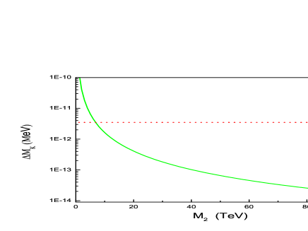
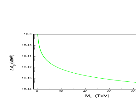
Figure 1: $\Delta M_{K}$ ( the left panel of the figure ) and $\Delta M_{D}$ ( the right panel of the figure ) as the function of $m_{2}$ the mass eigenvalue of the $h_{2}^{0}$.

IV.2 $D-\bar{D}$ mixing

The $D-\bar{D}$ mixing in our model is a little different form that of $K-\bar{K}$ mixing. The contributions to the $D-\bar{D}$ mixing come from box diagrams, which include the SM $W$ boson diagram, the two Higgs diagrams and the mixed diagrams. We assume the two Higgs diagrams dominant the contribution. The following are relevant vertices :

$$\left\{\matrix{\overline{c_{L}}d_{R}h^{+}_{i}:&&m_{d}v_{i}^{-1}{\cal U}^{*}_{i2}{\cal U}_{i1}\;,\cr\overline{c_{L}}s_{R}h^{+}_{i}:&&m_{s}v_{i}^{-1}{\cal U}^{*}_{i2}{\cal U}_{i2}\;,\cr\overline{c_{L}}b_{R}h^{+}_{i}:&&m_{b}v_{i}^{-1}{\cal U}^{*}_{i2}{\cal U}_{i3}\;,\cr}\right.\hskip 28.45274pt\left\{\matrix{\overline{u_{L}}d_{R}h^{+}_{i}:&&m_{d}v_{i}^{-1}{\cal U}^{*}_{i1}{\cal U}_{i1}\;,\cr\overline{u_{L}}s_{R}h^{+}_{i}:&&m_{s}v_{i}^{-1}{\cal U}^{*}_{i1}{\cal U}_{i2}\;,\cr\overline{u_{L}}b_{R}h^{+}_{i}:&&m_{b}v_{i}^{-1}{\cal U}^{*}_{i1}{\cal U}_{i3}\;,\cr}\right.$$ (21)

Then we have

$$M_{12}^{D}={1\over 384\pi^{2}}\Lambda^{2}f_{D}^{2}m_{D}\sum_{m}\sum_{n}y_{m}y_{n}\sum_{ij}{\cal Y}^{i}_{um}{\cal Y}_{cm}^{j*}{\cal Y}^{j}_{un}{\cal Y}^{i*}_{cn}{\cal I}(y_{m},y_{n},y_{i},y_{j})\;,$$ (22)

where $y_{\alpha},y_{\beta}=m_{\alpha,\beta}^{2}/\Lambda^{2}$ and ${\cal Y}_{mn}^{i}=v_{i}^{-1}{\cal U}_{im}^{*}{\cal U}_{in}$. The explicit expression of integration ${\cal I}(a,~{}b,~{}c,~{}d)$ can be found in Ref. grossmann .

Using $f_{D}=170~{}{\rm MeV}$ and $M_{D}=1864~{}{\rm MeV}$, we plotting in the right panel of Fig. 1 $\Delta M_{D}$ as a function of $m_{2}$. Our parameter settings are the same as that of the $K-\bar{K}$ mixing. the horizontal line in the figure represent the experimental value. We can read from the figure that the data of $D-\bar{D}$ mixing constraints the mass of $h_{2}^{+}$ to be no smaller than $4.2$ TeV.

IV.3 $B-\bar{B}$ mixing

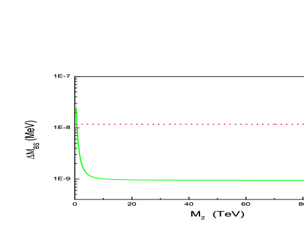
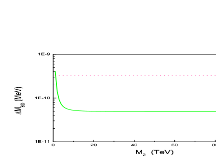
Figure 2: $\Delta M_{BS}$ ( the left panel of the figure) and $\Delta M_{BD}$ as the function of $m_{2}$ the mass eigenvalue of the $\phi_{2}^{0}$.

The mass difference in the neutral B meson system has been well measured by the D0 Collaboration and the CDF Collaboration at the Fermilab Tevatron. Similar to that of $K-\bar{K}$ mixing, there are also tree-level contributions to the $\Delta M_{B_{\alpha}}$. The following are relevant vertices that might lead to $B_{\alpha }-{\overline{B}}_{\alpha }$