Matter-wave chaos with a cold atom in a standing-wave laser field

Abstract

Coherent motion of cold atoms in a standing-wave field is interpreted as a propagation in two optical potentials. It is shown that the wave-packet dynamics can be either regular or chaotic with transitions between these potentials after passing field nodes. Manifestations of de Broglie-wave chaos are found in the behavior of the momentum and position probabilities and the Wigner function. The probability of those transitions depends on the ratio of the squared detuning to the Doppler shift and is large in that range of the parameters where the classical motion is shown to be chaotic.

1 Introduction

Cold atoms in a standing-wave laser field [1, 2, 3, 4, 5] are ideal objects for studying fundamental principles of quantum physics, quantum-classical correspondence, and quantum chaos. The proposal [6] to study atomic dynamics in a far-detuned modulated standing wave made atomic optics a testing ground for quantum chaos. A number of impressive experiments have been carried out in accordance with this proposal [7, 8, 9]. Furthermore, cold atoms have been recently used to study different phenomena in statistical physics including ratchet effect of a directed transport of atoms in the absence of a net bias [10, 11, 12] and Brillouin-like propagation modes in optical lattices [13].

New possibilities are opened if one works near the atom-field resonance where the interaction between the internal and external atomic degrees of freedom is intense. A number of nonlinear dynamical effects have been found [14, 15, 16] with point-like atoms in a near-resonant rigid optical lattice: chaotic Rabi oscillations, chaotic walking, dynamical fractals, Lévy flights, and anomalous diffusion.

Dynamical chaos in classical mechanics is a special kind of random-like motion without any noise and/or random parameters. It is characterized by exponential sensitivity of trajectories in the phase space to small variations in initial conditions and/or control parameters. Such sensitivity does not exist in isolated quantum systems because their evolution is unitary, and there is no well-defined notion of a quantum trajectory. Thus, there is a fundamental problem of emergence of classical dynamical chaos from more profound quantum mechanics which is known as quantum chaos problem and the related problem of quantum-classical correspondence. In a more general context it is a problem of wave chaos. It is clear now that quantum chaos, microwave, optical, and acoustic chaos have much in common (see [17] for a review). The common practice is to construct an analogue for a given wave object in a semiclassical (ray) approximation and study its chaotic properties (if any) by well-known methods of dynamical system theory. Then, it is necessary to solve the corresponding linear wave equation in order to find manifestations of classical chaos in the wave-field evolution in the same range of the control parameters. If one succeeds in that a quantum-classical or wave-ray correspondence is announced to be established.

In this paper we perform this program with cold two-level atoms in a one-dimensional standing-wave laser field and show that coherent dynamics of the atomic matter waves is really complicated in that range of the control parameters where the corresponding classical point-like atomic motion can be strictly characterized as a chaotic one. The effect is explained by a proliferation of atomic wave packets at the nodes of the standing wave.

2 Order and chaos in dynamics of atomic wave packets in a laser standing wave

The Hamiltonian of a two-level atom, moving in a one-dimensional classical standing-wave laser field, can be written in the frame rotating with the laser frequency $\omega_{f}$ as follows:

$$\hat{H}=\frac{\hat{P}^{2}}{2m_{a}}+\frac{\hbar}{2}(\omega_{a}-\omega_{f})\hat{\sigma}_{z}-\hbar\Omega\left(\hat{\sigma}_{-}+\hat{\sigma}_{+}\right)\cos{k_{f}\hat{X}},$$ (1)

where $\hat{\sigma}_{\pm,z}$ are the Pauli operators for the internal atomic degrees of freedom, $\hat{X}$ and $\hat{P}$ are the atomic position and momentum operators, $\omega_{a}$ and $\Omega$ are the atomic transition and Rabi frequencies, respectively. We will work in the momentum representation and expand the state vector as follows:

$${|\Psi(t)\closeket}=\int[a(P,t){|2\closeket}+b(P,t){|1\closeket}]{|P\closeket}dP,$$ (2)

where $a(P,t)$ and $b(P,t)$ are the probability amplitudes to find atom at time $t$ with the momentum $P$ in the excited and ground states, respectively. The Schrödinger equation for these amplitudes is

$$i\dot{a}(p) =\frac{1}{2}(\omega_{r}p^{2}-\Delta)a(p)-\frac{1}{2}[b(p+1)+b(p-1)],$$ (3)

$$i\dot{b}(p) =\frac{1}{2}(\omega_{r}p^{2}+\Delta)b(p)-\frac{1}{2}[a(p+1)+a(p-1)],$$

where dot denotes differentiation with respect to dimensionless time $\tau\equiv\Omega t$, and the atomic momentum $p$ is measured in units of the photon momentum $\hbar k_{f}$. The normalized recoil frequency, $\omega_{r}\equiv\hbar k_{f}^{2}/m_{a}\Omega$, and the atom-field detuning, $\Delta\equiv(\omega_{f}-\omega_{a})/\Omega$, are the control parameters.

We will treat the wave-packet motion in the dressed-state basis [18]

$${|+\closeket}_{\Delta}=\sin{\Theta}{|2\closeket}+\cos{\Theta}{|1\closeket},\ {|-\closeket}_{\Delta}=\cos{\Theta}{|2\closeket}-\sin{\Theta}{|1\closeket}.$$ (4)

The dressed states are eigenstates of an atom at rest in a laser field with the eigenvalues of the quasienergy $E_{\Delta}^{(\pm)}$ and the mixing angle $\Theta$:

$$E_{\Delta}^{(\pm)}=\pm\sqrt{\frac{\Delta^{2}}{4}+\cos^{2}{x}},\ \tan{\Theta}\equiv\frac{\Delta}{2\cos{x}}-\sqrt{\left(\frac{\Delta}{2\cos{x}}\right)^{2}+1}.$$ (5)

The depth of the nonresonant optical potential is

$$U_{\Delta}=\left|\sqrt{\frac{\Delta^{2}}{4}+1}-\frac{|\Delta|}{2}\right|.$$ (6)

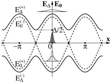
Figure 1: The resonant $E_{0}^{(\pm)}$ ($\Delta=0$, dotted curves) and non-resonant $E_{\Delta}^{(\pm)}$ ($\Delta\not=0$, solid curves) potentials of a two-level atom in a standing-wave laser field. An atomic wave packet, centered at $x_{0}=0$, and its initial evolution in the upper and lower potentials are shown schematically.

At $\Delta=0$, the depth changes abruptly from $1$ to $2$. The resonant $E_{0}^{(\pm)}$ ($\Delta=0$) and non-resonant $E_{\Delta}^{(\pm)}$ ($\Delta\not=0$) potentials of an atom in a standing-wave field are drawn in Fig. 1. The ground atomic state can be written as a superposition of the dressed states

$${|1\closeket}={|+\closeket}_{\Delta}\frac{1}{\sqrt{1+\tan^{2}{\Theta}}}-{|-\closeket}_{\Delta}\frac{\tan{\Theta}}{\sqrt{1+\tan^{2}{\Theta}}}.$$ (7)

In general, an atom in the ground state, placed initially at $x_{0}=0$, will move along two trajectories simultaneously because it is situated simultaneously at the top of $E_{\Delta}^{(+)}$ and the bottom of $E_{\Delta}^{(-)}$ (see Fig.1).

In the dressed-state basis, the probability amplitudes to find the atom at the point $x$ in the potentials $E_{\Delta}^{(+)}$ and $E_{\Delta}^{(-)}$ are, respectively,

$$C_{+}(x)=a(x)\sin{\Theta}+b(x)\cos{\Theta},\ C_{-}(x)=a(x)\cos{\Theta}-b(x)\sin{\Theta},$$ (8)

where the amplitudes in the bare-state basis, $a(x)$ and $b(x)$, are computed in the position representation with the help of the Fourier transform

$$a(x)={\rm const}\int_{-\infty}^{\infty}dp^{\prime}e^{ip^{\prime}x}a(p^{\prime}),\ b(x)={\rm const}\int_{-\infty}^{\infty}dp^{\prime}e^{ip^{\prime}x}b(p^{\prime}).$$ (9)

To clarify the character of the bipotential motion we write down the Hamiltonian of the internal degrees of freedom in the basis ${|\pm\closeket}=({|1\closeket}\pm{|2\closeket})/\sqrt{2}$:

$$\hat{H}_{\rm int}=\hat{\sigma}_{z}\cos x+\frac{\Delta}{2}\hat{\sigma}_{x}.$$ (10)

Let us linearize the potential in the vicinity of a node of the standing wave and estimate a small distance the atom makes when crossing the node as follows: $\delta x\simeq\omega_{r}|p_{\rm node}|\tau$, where $|p_{\rm node}|$ is the mean atomic momentum near the node. The quantity $\omega_{r}|p_{\rm node}|$ is a normalized Doppler shift for an atom moving with the momentum $|p_{\rm node}|$, i.e., $\omega_{D}\equiv\omega_{r}|p_{\rm node}|\equiv k_{f}|v_{\rm node}|/\Omega$. We arrive now at the famous Landau–Zener problem [19] to find a probability of transition between the states (4) when the energy difference varies linearly in time. In other words it is a a probability of transition from one potential to another or from one trajectory of motion to another. The asymptotic solution is

$$P_{\rm LZ}=\exp\left(-\frac{\pi\Delta^{2}}{\omega_{D}}\right).$$ (11)

There are three possibilities.

1. $\Delta^{2}\gg\omega_{D}$. The transition probability is exponentially small and an atom moves adiabatically along, in general, two trajectories without any transitions between them.

2. $\Delta^{2}\ll\omega_{D}$. The probability of a Landau-Zener transition is close to unity, and an atom changes the potential each time upon crossing any node, i.e., it moves mainly in the resonant potentials $E_{0}^{(\pm)}$.

3. $\Delta^{2}\simeq\omega_{D}$. The probabilities to change the potential or to remain in the same one upon crossing a node are of the same order. In this regime one may expect strong complexification of the wave function.

At large and small detunings, the translational motion splits into two independent motions in the potentials $E_{\Delta}^{(\pm)}$, and the wave-packet motion is regular in the first two cases. In the third case, the motion is complex because of a proliferation of wave packets at the nodes of the standing wave. We call such a motion as ”a chaotic” one by the reasons which will be clear in section 3. The switch between the regular and chaotic regimes of atomic motion can be easily performed by changing the detuning.

Our normalization enables to change dimensionless values of the recoil frequency $\omega_{r}$ and the detuning $\Delta$ varying the Rabi frequency $\Omega$. Working with a cesium atom at the transition $6S_{1/2}$ – $6P_{3/2}$ ($m_{a}=133$ a. u., $\lambda_{a}=852.1$ nm and $\nu_{\rm rec}\simeq 2$ KHz [20]), we have $\omega_{r}=10^{-3}$ at $\Omega=1$ MHz. Let the atom is initially prepared in the ground state as a Gaussian wave packet in the momentum space with $p_{0}=55$. The probability to find the atom with the momentum $p$ at time $\tau$ is ${\it P}(p,\tau)=|a(p,\tau)|^{2}+|b(p,\tau)|^{2}$.

To illustrate the difference between the regular and chaotic regimes of the wave-packet motion we take two values of the detuning, $\Delta=1$ and $\Delta=0.2$. At $\Delta=1$, the motion is expected to be adiabatic and regular because $\Delta^{2}\gg\omega_{D}=0.055$, and the Landau–Zener probability, $P_{\rm LZ}$, is exponentially small. At $\Delta=0.2$, one expects a much more complicated wave-packet motion with nonadiabatic transitions between the two potentials at the field nodes because $\Delta^{2}=0.04\simeq\omega_{D}$. Figure 2 shows the dependence of the mean atomic momentum $<p>$ over a large time scale in those two cases. In both the cases $<p>$ oscillates in a rather irregular way. The difference is that for an adiabatically moving wave packet, which we refer as a regular motion, the mean atomic momentum oscillates in a narrow range around $p_{0}=55$ (the upper curve in the figure). Whereas the range of its oscillations for a wave packet moving with nonadiabatic transitions at the field nodes, which we refer as a chaotic motion, is much more broad (the lower curve in the figure). It is a simple illustration of the two different regimes of the wave-packet propagation in terms of the classical variable.

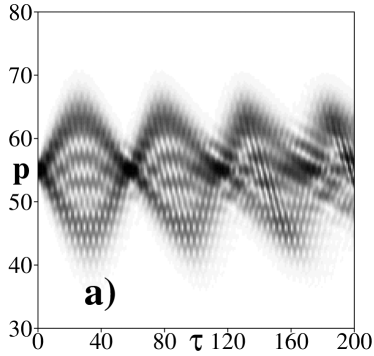
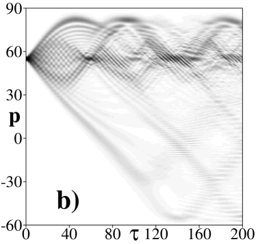
Figure 3: Momentum probability-density distribution ${\it P}(p,\tau)$ vs time in (a) the regular and (b) chaotic regimes of motion. The color codes the corresponding values of ${\it P}(p)$.

In Fig.  3a we plot the dependence of the momentum probability-density on time at $\Delta=1$. The initial wave packet splits from the beginning to a few components because the initial ground state is a superposition of the dressed states (4). The initial kinetic energy is enough to perform a ballistic motion. The momentum changes in a comparatively small range, from 40 to 70 of the photon-momentum units. The packet does not split at the nodes of the standing wave but it, on the contrary, recollects in the momentum space at the nodes and spreads in between. However, this recollection smears out in course of time.

At $\Delta=0.2$, the atomic ground state is the following superposition of the dressed states: ${|1\closeket}\simeq 0.74{|+\closeket}_{\Delta}+0.66{|-\closeket}_{\Delta}$. The ${|+\closeket}_{\Delta}$-component of the initial wave packet, i.e., that one, starting from the top of the potential $E_{\Delta}^{(+)}$, overcomes the barriers of that potential and moves in the positive direction of the axis $x$ proliferating at the nodes. As to the ${|-\closeket}$-component with decreased values of $p$, it will be trapped in the potential well performing oscillations in the momentum and position spaces. The period of those oscillations is about $T\simeq 280$ which is equal approximately to the period of revivals of the Rabi oscillations for the population inversion. Figure 3b illustrates the effect of simultaneous trapping and ballistic motion of the atomic wave packet in the chaotic regime resulting in a broad momentum distribution, from $p=-60$ to $p\simeq 80$.

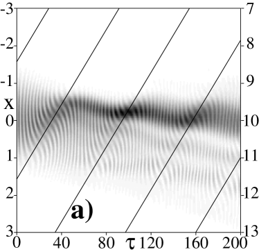
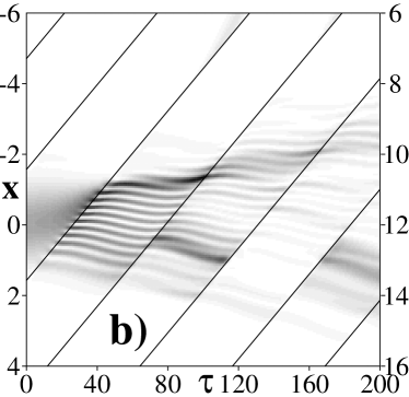
Figure 4: The probability $|C_{-}(x)|^{2}$ to find the atom in the potential $E_{\Delta}^{(-)}$ in the moving frame of reference in (a) the regular and (b) chaotic regimes of motion. The slopes mark positions of the nodes in the moving frame and the color codes the values of $|C_{-}(x)|^{2}$.

To illustrate the nonadiabatic transitions from one potential to another and their absence at the nodes more explicitly, we go to the position space and compute the probabilities $|C_{\pm}(x,\tau)|^{2}$ (8) to be at the point $x$ at time $\tau$ in the potentials $E_{\Delta}^{(+)}$ and $E_{\Delta}^{(-)}$, respectively. In Fig. 4 we plot the evolution of the probability density $|C_{-}(x,\tau)|^{2}$ in the frame moving with the initial atomic velocity $\omega_{r}p_{0}=0.055$. The slope straight lines in the figure mark positions of the nodes in the moving frame. In the case of the regular motion at $\Delta=1$ (Fig. 4a), no transitions happen when the atom crosses the nodes. In the chaotic regime at $\Delta=0.2$, one observes visible changes in the probability-density $|C_{-}(x)|^{2}$ exactly at the node lines (see Fig. 4b). It means transitions from one trajectory to another at the field nodes that should occur in a specific range of the control parameters if $\Delta^{2}\simeq\omega_{D}$. This results in a proliferation of the components of the wave packet at the nodes and, therefore, a complexification of the wave function (see Fig. 3b).

The Wigner function can be used to visualize complexity of the wave function in the chaotic regime of the atomic motion. We compute the evolution of the Wigner function of the ground state in the momentum space

$$W_{b}(p,x,\tau)={\rm const}\int_{-\infty}^{\infty}dp^{\prime}e^{-ip^{\prime}x}a(p-p^{\prime}/2)a^{*}(p+p^{\prime}/2).$$ (12)

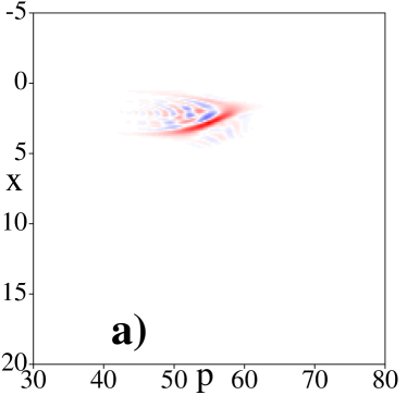
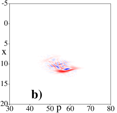
Figure 5: Contour plots of the Wigner function at (a) $\tau=50$ and (b) $\tau=200$ for the regular regime of the atomic motion. Color online: red and blue areas show positive and negative values of the Wigner function, respectively.

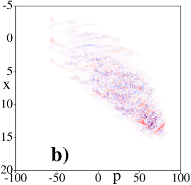
Figure 6: The same as in Fig. 5 for the chaotic regime of motion.

This quantity gives a quasi-probability distribution corresponding to a general quantum state (2). Figure 5 shows a contour plot of the Wigner function (12) at two moments of time, $\tau=50$ and $\tau=200$, when the atom moves in a regular way ($\Delta=1$). Figure 6 is a contour plot of this function at the same times, but with an atom making nonadiabatic transitions at the field nodes ($\Delta=0.2$). In the chaotic regime (Fig. 6b) we see a dust-like distribution of nonzero values of the Wigner function at $\tau=200$ which occupy much more larger area in the phase space than the function for the regular motion (Fig. 5b).

3 Quantum-classical correspondence

In this section we compare the results of the quantum treatment with those obtained for the same problem in the semiclassical approximation when the translational motion has been treated as a classical one [14, 15]. We must compare quantum results for a single atomic wave packet not with a single point-like atom but with an ensemble of point-like atoms. Dynamical chaos has been found and analyzed in detail in Refs. [14, 15] in the semiclassical approximation. Both the internal and external degrees of freedom of a two-level atom in a standing wave field have been shown to be chaotic in a specific range of values of the detuning $\Delta$, the recoil frequency $\omega_{r}$, and the initial momentum $p_{0}$.

Coherent semiclassical evolution of a point-like two-level atom is governed by the Hamilton-Schrödinger equations with the same normalization as in the quantum case [15]

$$\begin{gathered}\dot{x}=\omega_{r}p,\quad\dot{p}=-u\sin x,\quad\dot{u}=\Delta v,\\ \dot{v}=-\Delta u+2z\cos x,\quad\dot{z}=-2v\cos x,\end{gathered}$$ (13)

where

$$u\equiv 2\operatorname{Re}(a_{0}b_{0}^{*}),\ v\equiv-2\operatorname{Im}(a_{0}b_{0}^{*}),\ z\equiv|a_{0}|^{2}-|b_{0}|^{2}$$ (14)

are the atomic-dipole components ($u$ and $v$) and population-inversion ($z$), and $a_{0}$ and $b_{0}$ are the complex-valued probability amplitudes to find the atom in the excited, ${|2\closeket}$, and ground, ${|1\closeket}$, states, respectively. The system (13) has two integrals of motion, the total energy

$$W\equiv\frac{\omega_{r}}{2}p^{2}-u\cos x-\frac{\Delta}{2}z,$$ (15)

and the length of the Bloch vector, $u^{2}+v^{2}+z^{2}=1$. Equations (13) constitute a nonlinear Hamiltonian autonomous system with two and half degrees of freedom and two integrals of motion.

In classical mechanics there is a qualitative criterion of dynamical chaos, the maximal Lyapunov exponent $\lambda$, which measures the mean rate of the exponential divergence of initially closed trajectories in the phase space. In Fig. 7 we plot this quantity, computed with semiclassical equations of motion (13) vs the detuning $\Delta$ at $\omega_{r}=10^{-3}$ and $p_{0}=55$. At zero detuning, the set of semiclassical equations acquires an additional integral of motion and becomes integrable. The center-of-mass motion is regular at small values of the detuning, $\Delta\ll 1$, and at large ones, $\Delta>0.8$. Positive values of $\lambda$ at $0<\Delta<0.8$ characterize unstable motion. Local instability of the center-of-mass motion produce chaotic motion of an atom in a rigid standing wave without any modulation of its parameters in difference from the situation with atoms in a periodically kicked optical lattice [7, 8]. There is a range of initial conditions and the control parameters where the center-of-mass motion in an absolutely deterministic standing wave resembles a random walking. It means that a point-like atom alternates between flying through the lattice, and being trapped in its wells changing the direction of motion in a random-like way [15, 16].

In Fig. 8 we illustrate semiclassical chaos with the Poincaré mapping for a number of atomic ballistic trajectories in the western ($u<0$) and eastern ($u>0$) hemispheres of the Bloch sphere $(u,v,z)$ on the plane $v-z$. One can see a typical structure with regions of regular motion in the form of islands and chains of islands filled by regular trajectories. The islands are imbedded into a stochastic sea, and they are produced by nonlinear resonances of different orders. Increasing the resolution of the mapping, one can see that large islands are surrounded by islands of a smaller size each of which, in turn, is surrounded by a chain of even more smaller islands, and so on.

In quantum mechanics there is no well-defined notion of a trajectory in the phase space, the very phase space is not continuous due to the Heisenberg uncertainty relation, and, hence, the Lyapunov exponents can not be computed (however, see Ref. [21] where a notion of a Lyapunov exponent for quantum dynamics has been discussed). The main result of this paper is the establishment of the fact, that chaotically-like complexification of the wave function, caused by nonadiabatic transitions at the field nodes, occurs exactly at the same range of the control parameters where the semiclassical dynamics has been shown to be chaotic in Refs. [14, 15]. It should be stressed that quantum motion of a wave packet with nonadiabatic transitions between the two optical potentials is compared with the center-of-mass motion of an ensemble of atoms each of which moves in a single optical potentials. So, when we say about a quantum-classical correspondence we mean a correspondence between the wave function of a single quantum atom and the trajectories of the ensemble of classical atoms with different values of the initial momentum $p_{0}$ and at the other equal conditions.

4 Conclusion

We have studied coherent dynamics of cold atomic wave packets in a one-dimensional standing-wave laser field. The problem has been considered in the momentum representation and in the dressed-state basis where the motion of a two-level atom was interpreted as a propagation in two optical potentials. The character of that motion has been shown to depend strongly on the ratio of the squared detuning, $\Delta^{2}$, to the normalized Doppler shift $\omega_{D}$. In the regular regime, when $\Delta$ is comparatively large or small, wave packets move in a simple way. The chaotic regime occurs if $\Delta^{2}\simeq\omega_{D}$ when the probability for an atom to make nonadiabatic transitions while crossing the nodes of the standing wave is large. Atom in this regime of motion simultaneously moves ballistically and is trapped in a well of the optical potential. This type of motion and proliferation of wave packets at the nodes result in a complexification of the wave function both in the momentum and position spaces manifesting itself in the irregular behavior of the Wigner function.

Comparing the results of the quantum treatment with those obtained in the semiclassical approximation, when the translational motion has been treated as a classical one [14, 15], we have found that the wave-packet dynamics is complicated exactly in that range of the atom-field detuning and recoil frequency where the classical center-of-mass motion has been shown to be chaotic in the sense of exponential sensitivity to small variations in initial conditions or parameters.

As to possible practical applications of the results obtained we mention atomic lithography to produce small-scale complex prints of cold atoms (see, for example, beautiful experiments on coherent matter-wave manipulation [22, 23, 24]), new ways to manipulate atomic motion in optical lattices by varying the atom-filed detuning and atomic ratchets with cold atoms.

Figure 2: Mean atomic momentum $\left<p\right>$ vs time in the regular ($\Delta=1$, the upper bold curve) and chaotic ($\Delta=0.2$) regimes of motion.

Figure 7: Maximal Lyapunov exponent $\lambda$, computed with semiclassical equations of motion (13), vs the detuning $\Delta$ at $\omega_{r}=10^{-3}$ and $p_{0}=55$.

Figure 8: Poincaré sections of the Bloch sphere illustrating the effect of semiclassical chaos with point-like atoms at $\omega_{r}=10^{-5}$, $\Delta=-0.05$ and the total atomic energy $W=36.45$. (a) $u<0$ (western Bloch hemisphere), (b) $u>0$ (eastern Bloch hemisphere).

References

- [1] V.G. Minogin, V.S. Letokhov, Laser Light Pressure on Atoms, Gordon and Breach, New York, 1987.
- [2] A.P. Kazantsev, G.I. Surdutovich, V.P. Yakovlev, Mechanical Action of Light on Atoms, Singapore, World Scientific, 1990.
- [3] P. Meystre, Atom Optics, New York, Springer-Verlag, 2001.
- [4] W.P. Schleich, Quantum Optics in Phase Space, New York, Wiley, 2001.
- [5] M.V. Fedorov, M.A. Efremov, V.P. Yakovlev, W.P. Schleich, JETP 97 (2003) 522 [Zh. Eksp. Teor. Fiz. 124 (2003) 578].
- [6] R. Graham, M. Schlautmann, P. Zoller, Phys. Rev. A 45 (1992) R19 .
- [7] M.G. Raizen, Adv. At. Mol. Opt. Phys. 41 (1999) 43. D.A. Steck, et al, Science 293 (2001) 274.
- [8] W.K. Hensinger, N.R. Heckenberg, G.J. Milburn, H. Rubinsztein-Dunlop, J. Opt. B: Quantum Semiclass. Opt. 5 (2003) 83.
- [9] M. Sadgrove, S. Wimberger, S. Parkins, and R. Leonhardt, Phys. Rev. Lett. 94, (2005) 174103.
- [10] C. Mennerat-Robilliard et al, Phys. Rev. Lett. 82, (1999) 851.
- [11] M. Schiavoni, L. Sanchez-Palencia, F. Renzoni, G. Grynberg, Phys. Rev. Lett. 90, (2003) 094101.
- [12] G. G. Carlo, G. Benenti, G. Casati, S. Wimberger, O. Morsch, R. Manella, E. Arimondo, Phys. Rev. A 74, (2006) 033617.
- [13] L. Sanchez-Palencia, F. R. Carminati, M. Schiavoni, F. Renzoni, G. Grynberg, Phys. Rev. Lett. 88, (2002) 133903.
- [14] S.V. Prants, JETP Letters 75 (2002) 651. [Pis’ma ZhETF 75, 777 (2002)].
- [15] V.Yu. Argonov, S.V. Prants, Phys. Rev. A 75 (2007) art. 063428.
- [16] V.Yu. Argonov, S.V. Prants, Phys. Rev. A 78 (2008) art. 043413.
- [17] D. Makarov, S. Prants, A. Virovlyansky, G. Zaslavsky, Ray and wave chaos in ocean acoustics, Singapore, World Scientific, 2010.
- [18] C. Cohen-Tannoudji, J. Dupon-Roc, G. Grynberg, Atom-Photon Interaction, Weinheim, Wiley, 1998.
- [19] L. Landau, Phys. Z. Sowjetunion 2 (1932) 46. C. Zener, Proc. R. Soc. London A 2 (1932) 137.
- [20] C.S. Adams, M. Sigel, J. Mlynek, Phys. Rep. 240 (1994) 143.
- [21] V.I. Man’ko, R.V. Mendes, Physica D 145 330 (2000) 330.
- [22] G. Zabow, R.S. Conroy, M. G. Prentiss, Phys. Rev. Lett. 92, (2004) 180404.
- [23] A. Zenesini, H. Lignier, D. Ciampini, O. Morsch, E. Arimondo, Phys. Rev. Lett. 102, (2009) 100403.
- [24] S. Wu, A. Tonyushkin, M. G. Prentiss, Phys. Rev. Lett. 103, (2009) 034101.