Group-theoretical approach to study atomic motion in a laser field

Abstract

Group-theoretical approach is applied to study behavior of lossless two-level atoms in a standing-wave laser field. Due to the recoil effect, the internal and external atomic degrees of freedom become coupled. The internal dynamics is described quantum mechanically in terms of the $SU(2)$ group parameters. The evolution operator is found in an explicit way after solving a single ODE for one of the group parameters. The translational motion in a standing wave is governed by the classical Hamilton equations which are coupled to the $SU(2)$ group equations. It is shown that the full set of equations may be chaotic in some ranges of the control parameters and initial conditions. It means physically that there are regimes of motion with chaotic center-of-mass motion and irregular internal dynamics. It is established that the chaotic regime is specified by the character of oscillations of the group parameter characterizing the mean interaction energy between the atom and the laser field. It is shown that the effect of chaotic walking can be observed in a real experiment with cold atoms crossing a standing-wave laser field.

1 Introduction

In quantum physics the unitary time evolution of a driven quantum system is described by the evolution operator equation

$$i\hbar\frac{d}{dt}\hat{U}(t,t_{0})=\hat{H}\left[{\bf h}(t)\right]\hat{U}(t,t_{0}),\quad\hat{U}(t_{0},t_{0})=\hat{I},$$ (1)

where $\hat{U}_{{\bf h}}(t,t_{0})$ is a time evolution operator, $\hat{H}$ is a Hamiltonian and ${\bf h}(t)$ is a vector-function of the system’s control parameters. From the abstract point of view, the evolution equation (1) can be regarded as a differential equation on the group of dynamical symmetry. By dynamical symmetry we mean simply that the Hamiltonian can be expressed as a linear combination of operators belonging to a finite-dimensional Lie algebra with $n$ basic elements. The parameters, $g_{k}\,,k=1,2,\ldots,n$, of the respective Lie group satisfy to a set of $n$ first-order ordinary differential nonlinear equations which depend only on the structure of the algebra and on $c$-number coefficients of the system’s Hamiltonian or the other governing operator [1, 2, 3, 4]. Thus, the dynamical group itself may be considered as a dynamical system.

The dynamical-symmetry and Lie-algebraic approach has been successfully applied to describe the time evolution of numerous physical systems in different disciplines extending from classical mechanics [5], classical optics [6, 7, 8, 9] and quantum mechanics [10, 11, 12, 13, 14] to physics of neutrino oscillations [15]. As to study of dynamics of laser driven atoms, this approach has been applied to get Lie algebraic solution of the Bloch equations [16, 17].

The evolution of an isolated quantum system is regular, and the overlap of any two different quantum state vectors is a constant in course of time. All the expectation values of the quantum variables evolve in a quasiperiodic way at most. It does no matter how complicated is a dynamical symmetry of the quantum system under consideration and the corresponding Lie algebra. On the other hand, it is well known that even simple classical systems may be unstable and demonstrate chaotic behavior [19, 20]. Classical instability is usually defined as an exponential separation of two initially close trajectories in time with an asymptotic rate given by the maximal Lyapunov exponent $\lambda$. Such a behavior is possible because of the continuity of the classical phase space where the system’s states can be arbitrary close to each other. The trajectory concept is absent in quantum mechanics, and the quantum phase space is not continuous due to the Heisenberg uncertainty principle. Perfectly isolated quantum systems are unitary, and there can be no chaos in the sense of exponential instability even if their classical limits are chaotic. What is usually understood under quantum chaos is, in essence, the special features of the quantum unitary evolution of the system under consideration (no matter how complicated the evolution is) in the region of its control parameter values and/or initial conditions at which its classical analogue is chaotic [21, 22, 23, 24]. In fact, it is not a special quantum problem. Any type of propagating waves (electromagnetic, sound or others), satisfying to a linear wave equation (which is an analogue of the Scrodinger equation), has the same property. Wave chaos is the special features of the wave field in the region of control parameters and/or initial conditions at which its ray analogue is chaotic [25, 26]. Thus, the quantum (wave) chaos problem is partly the problem of quantum (wave)-classical (ray) correspondence.

Let us describe briefly the interconnection between the dynamical symmetries and dynamical chaos in physics of the atom-field interaction.

1. The simplest problem is dynamics of a two-level atom at rest in an external laser field. From the dynamical symmetry point of view, the $SU(2)$ group, generated by the corresponding Hamiltonian, is driven by an external force that is not considered to be a dynamical system. It is the case of an external driving. The problem has been studied in Ref. [4] where it has been shown that the evolution of atomic internal variables in a linearly polarized bichromatic laser field with incommensurate frequencies may be very complicated on the Bloch sphere albeit regular. It is simply because the dynamics takes place on the two-dimensional surface of the Bloch sphere.

2. If we deal with a two-level atom at rest in an ideal cavity and take into account the response of the atom to the cavity radiation field, the semiclassical evolution of the coupled atom-field system may be chaotic in the sense of exponential sensitivity to small variations in initial conditions and/or parameters [27, 28, 29, 30, 31, 32, 33]. This is the case of so-called dynamical driving [4] when the $SU(2)$ group, generated by the atomic Hamiltonian, is driven by another dynamical system, the field one. We deal now with a quantum system, the atom, which is coupled with a classical system, the radiation field governed by the Maxwell equations. The resulting Maxwell-Scrodinger (Bloch) equations constitute the five-dimensional set of nonlinear ordinary differential equations with two integrals of motion, the total atom-field energy (which is a constant in the absence of any losses) and the length of the Bloch vector. The motion in the phase space takes place on a three-dimensional manifold and may be chaotic due to transverse intersection of stable and unstable manifolds of hyperbolic points in some ranges of the control parameters, the values of the maximal Rabi frequency and the coupling strength [33].

3. If a two-level atom moves within a standing-wave laser field in an open space, not in a cavity, the field may be considered as an external driving but one needs to take into account the atomic recoil effect, i.e. changes of the atomic momentum after absorption or emission photons. If the atom is not especially cold, we may treat its translation degree of freedom classically. It is again the case of the dynamical driving with the $SU(2)$ group driven by the dynamical system which is now the classical atomic degree of freedom. The governing Hamilton-Scrodinger equations constitute the five-dimensional set of nonlinear ordinary differential equations with two integrals of motion, the atomic total energy, including the kinetic one, and the length of the Bloch vector. The motion in the phase space takes place on a three-dimensional manifold and may be chaotic in some ranges of the control parameters, the values of the maximal Rabi and atomic recoil frequencies. A number of nonlinear dynamical effects have been analytically and numerically demonstrated with this system: chaotic Rabi oscillations [34, 35], Hamiltonian chaotic atomic transport and dynamical fractals [36, 37, 38], Lévy flights and anomalous diffusion [39, 35]. These effects are caused by local instability of the center-of-mass motion in a laser field. A set of atomic trajectories under certain conditions becomes exponentially sensitive to small variations in initial quantum internal and classical external states or/and in the control parameters, mainly, the atom-laser detuning.

In this paper we consider the physical situation mentioned in the third part of our nomenclature to focus at the ultimate reasons of chaotic atomic external and internal motion and its connection with the $SU(2)$ dynamical symmetry.

2 Lie algebraic solution for the evolution operator with the $SU(2)$ dynamical symmetry

In a variety of physical problems $SU(2)$ appears to be a group of dynamical symmetry. It is known [1, 4] that the set of three equations for the $SU(2)$ group parameters can be reduced to a single second-order differential equation. The form of this governing equation depends on the choice of the basis and its exponential ordering. The appropriate choice of parameterization of the dynamical group is especially important if we need to solve explicitly the governing equation for a given physical Hamiltonian.

The Hermitian Hamiltonian of a quantum system with the $SU(2)$ dynamical symmetry can be cast in the general form

$$\hat{H}(t)=h_{0}(t)\hat{R}_{0}+h^{*}(t)\hat{R}_{-}+h(t)\hat{R}_{+},$$ (2)

where $\hat{R}_{0}$ and $\hat{R}_{\pm}$ are the generators that satisfy the commutation relations

$$\left[\hat{R}_{-},\hat{R}_{+}\right]=-2\hat{R}_{0},\quad\left[\hat{R}_{0},\hat{R}_{\pm}\right]=\pm\hat{R}_{\pm}.$$ (3)

It is convenient to choose the following noncanonical parameterization of the $SU(2)$ group

$$\hat{U}=\exp\Bigl{[}\Bigl{(}g_{0}-i\int\limits_{0}^{t}h_{0}\,d\tau\Bigr{)}\hat{R}_{0}\Bigr{]}\;\exp g_{-}\hat{R}_{-}\;\exp g_{+}\hat{R}_{+}\;.$$ (4)

Substituting Eq.(4) into Eq.(1), one finds the set of differential equations for the group parameters that can be reduced to the single equation for the group parameter $g\equiv\exp(g_{0}/2)$

$$\frac{d^{2}g}{dt^{2}}-\Bigl{(}\frac{{dh}/{dt}}{h}+ih_{0}\Bigr{)}\frac{dg}{dt}+\mid h\mid^{2}g=0\;,\;g(0)=1\;,\;\frac{dg}{dt}(0)=0\;.$$ (5)

Once Eq.(5) is solved analytically, all the other parameters in the product (4) may be expressed in terms of the parameter $g$ as follows:

$$g_{-}=\frac{ig({dg}/{dt})}{h}\exp\Bigl{(}-i\int\limits_{0}^{t}h_{0}\,d\tau\Bigr{)}\;,\quad\frac{{dg}_{+}}{dt}=-\frac{ih}{g^{2}}\exp\Bigl{(}i\int\limits_{0}^{t}h_{0}\,d\tau\Bigr{)}\;.$$ (6)

It is convenient to introduce the new variable

$$\tilde{g}\equiv g_{-}/g.$$ (7)

Then any group element in the parameterization (4) can be described by a pair of complex numbers $g$ and $\tilde{g}$ obeying the condition

$$\mid{g\mid}^{2}+\mid{\tilde{g}\mid}^{2}=1\;.$$ (8)

It should be noted that all these formulas are valid within any representation and within any realization of the $SU(2)$ group. It is well known that the unitary irreducible representations of $SU(2)$ are characterized by half-integer and integer numbers $j$. The dimensionality of the $j$th representation is equal to $2j+1$. In the $(2j+1)$-dimensional space of representation there is a canonical basis

$$\left|j,m\right\rangle,\quad m=-j,-j+1,...,j\;.$$ (9)

The representation matrix elements in the noncanonical parameterization (4) are given by [4]

$$\begin{array}[]{c}U_{m^{\prime}m}^{(j)}=\exp\left[-im^{\prime}\int\limits_{0}^{t}h_{0}(\tau)d\tau\right]\sum\limits_{l=-j}^{j}\left[\frac{(j-m^{\prime})!(j-m)!}{(j+m^{\prime})!(j+m)!}\right]^{1/2}\times\\ \frac{(j+l)!}{(j-l)!(l-m)!(l-m^{\prime})!}g^{m+m^{\prime}}({\tilde{g}})^{l-m^{\prime}}(-{\tilde{g}^{*}})^{l-m}\;.\end{array}$$ (10)

To analyze the dynamics of a two-level quantum system we need the two-dimensional representation of the $SU(2)$ group. In this case the generators $R$’s are connected with the familiar Pauli matrices

$$\hat{R}_{0}=\frac{1}{2}\hat{\sigma}_{z}=\frac{1}{2}\left|\begin{array}[]{cc}1&0\\ 0&-1\end{array}\right|,\quad\hat{R}_{-}=\hat{\sigma}_{-}=\left|\begin{array}[]{cc}0&0\\ 1&0\end{array}\right|,\quad\hat{R}_{+}=\hat{\sigma}_{+}=\left|\begin{array}[]{cc}0&1\\ 0&0\end{array}\right|\;,$$ (11)

where

$$[\hat{\sigma}_{+},\,\hat{\sigma}_{-}]=\hat{\sigma}_{z}\;,\quad[\hat{\sigma}_{z},\,\hat{\sigma}_{\pm}]=\pm 2\hat{\sigma}_{\pm}\;.$$ (12)

In this representation the Hamiltonian of a driven two-level system has the form

$$\hat{H}(t)=\frac{1}{2}\hbar\omega_{a}\hat{\sigma}_{z}+\hbar\Omega^{*}(t)\hat{\sigma}_{-}+\hbar\Omega(t)\hat{\sigma}_{+}\;,$$ (13)

where $\Omega(t)$ is a time-dependent function which is, in general, a complex-valued one. The temporal evolution of the two-level system is now governed by the equation

$$\frac{d^{2}g}{dt^{2}}-\Bigl{(}\frac{{d\Omega}/{dt}}{\Omega}+i\omega_{a}\Bigr{)}\frac{dg}{dt}+\mid\Omega\mid^{2}g=0\;,\;g(0)=1\;,\;\frac{dg}{dt}(0)=0\;.$$ (14)

The evolution matrix in the basis

$${\left|1\right>}={\left|\frac{1}{2}\;,-\frac{1}{2}\right>},{\left|2\right>}={\left|\frac{1}{2}\;,\frac{1}{2}\right>}$$ (15)

is given by

$$\hat{U}^{(1/2)}=\left(\begin{array}[]{cc}e^{-i\omega_{a}t/2}&0\\ 0&e^{i\omega_{a}t/2}\end{array}\right)\left(\begin{array}[]{cc}g&-{\tilde{g}}^{*}\\ {\tilde{g}}&g^{*}\end{array}\right)\;.$$ (16)

3 The $SU(2)$ group–Hamilton equations for a two-level atom moving in a standing-wave laser field

We consider a two-level atom with mass $m_{a}$ and transition frequency $\omega_{a}$, moving with the momentum $P$ along the axis $X$ in a one-dimensional classical laser standing wave with the frequency $\omega_{f}$ and the wave vector $k_{f}$. In the frame, rotating with the frequency $\omega_{f}$, the model Hamiltonian is the following:

$$\hat{H}=\frac{P^{2}}{2m_{a}}+\frac{1}{2}\hbar(\omega_{a}-\omega_{f})\hat{\sigma}_{z}-\hbar\Omega_{0}\left(\hat{\sigma}_{-}+\hat{\sigma}_{+}\right)\cos{k_{f}X},$$ (17)

where $\Omega_{0}$ is the maximal Rabi frequency which is proportional to the square root of the number of photons in the wave. The laser field is assumed to be strong enough, so we can treat the field classically.

In the process of emitting and absorbing photons, atoms not only change their internal electronic states but their external translational states change as well due to the photon recoil. If the atomic mean momentum is large as compared to the photon momentum $\hbar k_{f}$, one can describe the translational degree of freedom classically. The position and momentum of a point-like atom satisfy classical Hamilton equations of motion which we represent in the normalized form

$$\dot{x}=\omega_{r}p,\quad\dot{p}=-<\hat{\sigma}_{-}(t)+\hat{\sigma}_{+}(t)>\sin x,$$ (18)

where $x\equiv k_{f}X$ and $p\equiv P/\hbar k_{f}$ are normalized classical atomic center-of-mass position and momentum, respectively. The dot denotes differentiation with respect to the dimensionless time $\tau\equiv\Omega_{0}t$ and $\omega_{r}\equiv\hbar k_{f}^{2}/m_{a}\Omega_{0}\ll 1$ is the normalized recoil frequency. To compute the quantum expectation value $<\hat{\sigma}_{-}(t)+\hat{\sigma}_{+}(t)>$ we need to use the solution for the evolution operator (16). Supposing that the atom is initially in the ground state ${\left|1\right>}$, we get

$$<\hat{\sigma}_{-}(t)+\hat{\sigma}_{+}(t)>={\left<1\right|}\hat{U}^{\dagger}(t)\hat{U}(t){\left|1\right>}=-(gG^{*}+g^{*}G),$$ (19)

where we introduce for convenience the new complex-valued variable

$$G\equiv-\frac{i\dot{g}^{*}}{\cos x}.$$ (20)

The internal atomic dynamics is governed by Eq. (14) that can be rewritten in the form of two first-order equations for the complex-valued group parameters $g$ and $G$. The self-consistent set of equations for the coupled external and internal atomic degrees of freedom now reads as

$$\dot{x}=\omega_{r}p,\quad\dot{p}=(gG^{*}+g^{*}G)\sin x,\\ \dot{g}=iG\cos x,\quad\dot{G}=-i\Delta G+ig\cos x,$$ (21)

where the normalized recoil frequency $\omega_{r}$ and the atom-field detuning, $\Delta\equiv(\omega_{f}-\omega_{a})/\Omega_{0}$, are the control parameters. The six-dimensional dynamical system (21) has two independent integrals of motion, the total energy,

$$H\equiv\frac{\omega_{r}}{2}p^{2}+(gG^{*}+g^{*}G)\cos x-\frac{\Delta}{2}(GG^{*}-gg^{*}),$$ (22)

and the integral,

$$\mid{g\mid}^{2}+\mid{G\mid}^{2}=1$$ (23)

reflecting conservation of the norm of the atomic wave function. It is evident from the second integral (23) that the squared absolute values of the $SU(2)$ group parameters, $\mid{g\mid}^{2}$ and $\mid{G\mid}^{2}$, have the sense of the probability amplitudes to find the atom in the ground and excited states, respectively.

The equations of motion (21) describe the mixed quantum-classical dynamics of a two-level atom in a one-dimensional standing-wave laser field. The dynamical $SU(2)$ group is responsible for internal atomic dynamics caused by the interaction of the atomic electric dipole moment with the strength of the electric component of the field. The quantum expectation value of the corresponding interaction energy is given by the combination of the $SU(2)$ group parameters (19). The classical translational degree of freedom is described by the Hamilton equations (see the first two equations in the set (21)) governed by the interaction energy. In Introduction we called such a situation as a dynamical driving when the $SU(2)$ group, generated by the atomic quantum Hamiltonian, is driven by another dynamical system, the classical atomic degree of freedom. In fact, we deal not with a fully quantum system but with a quantum-classical hybrid which is described by the c-number nonlinear dynamical system (21) that may be chaotic in the strict sense of this term in some ranges of the control parameters and/or initial conditions.

4 Dynamical chaos in the group-theoretical picture

Equations (21) constitute a nonlinear autonomous dynamical system with three degrees of freedom and, in general, with the two integrals of motion, (22) and (23). Thus, the dynamical system (21) may be chaotic in the sense of exponential sensitivity to small variation in initial conditions and/or the control parameters, $\omega_{r}$ and $\Delta$. The common test to confirm that is to compute the maximum Lyapunov exponent characterizing the mean rate of exponential divergence of initially close trajectories which serves as a quantitative measure of dynamical chaos [40, 41]:

$$\lambda({\bf Q}_{0},\Delta{\bf q}_{0})=\lim_{t\to\infty,\Delta{\bf q}_{0}\to 0}\frac{1}{t}\ln\frac{\left\|\Delta{\bf q}({\bf Q}_{0},t)\right\|}{\left\|\Delta{\bf q}_{0}\right\|},$$ (24)

where $\Delta{\bf q}$ is the vector in the phase space with the components $\left\{\Delta q_{j},j=1,...,N\right\}$ and the norm $\left\|\Delta{\bf q}\right\|$. In Eq.(24), $\Delta{\bf q}_{0}$ and $\Delta{\bf q}({\bf Q}_{0},t)$ denote the separation between two initially adjacent trajectories at the initial moment $t=0$ and at time $t$, respectively, ${\bf Q}_{0}$ is the initial position. If, at least, one of the Lyapunov exponents of the dynamical system under question is positive, then trajectories, starting close together in the phase space, separate exponentially as time grows. This very sensitive dependence on initial conditions is one of the main indicator of dynamical chaos.

The result of computation of the maximum Lyapunov exponent with the equations of motion (21) at $\omega_{r}=10^{-3}$ in dependence on the detuning $\Delta$ and the initial atomic momentum $p_{0}$ is shown in Fig. 1. Color in the plot codes the value of the maximum Lyapunov exponent $\lambda$. In white regions in Fig. 1 the values of $\lambda$ are almost zero, and the atomic motion is regular in the corresponding ranges of $\Delta$ and $p_{0}$. In shadowed regions positive values of $\lambda$ imply unstable motion. The atoms with zero $\lambda$’s either oscillate in a regular way in a well of the optical potential or move ballistically over the hills of the potential with a regular variation of their velocity.

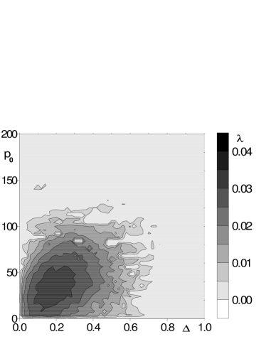
Figure 1: Maximum Lyapunov exponent, $\lambda$, vs the atom-field detuning $\Delta$ (in units of the maximal Rabi frequency $\Omega$) and the initial atomic momentum $p_{0}$ (in units of the photon momentum $\hbar k_{f}$) at $\omega_{r}=10^{-3}$. Color codes the values of $\lambda$.

Figure 2: Regimes of motion of two-level atoms in a one-dimensional deterministic standing-wave laser field. Trajectories in the real space at $\omega_{r}=10^{-3}$: regular flight (RF, $\Delta=0.8$, $p_{0}=45$), chaotic flight (CF, $\Delta=0.2$, $p_{0}=45$), chaotic walking (CW, $\Delta=0.2$, $p_{0}=10$) and trapping in a potential well (T, $\Delta=-0.2$, $p_{0}=5$). $x$ is in units of the wavelength $\lambda_{f}$.

Figure 3: Plots with 50 atomic trajectories with different values of the initial atomic momentum $0\leq p_{0}\leq 50$ but with the same initial position $x_{0}=0$ and the same other initial conditions. (a) Real space. (b) Momentum space.

At exact resonance, the equations of motion (21) become integrable due to an additional integral of motion, $gG^{*}+g^{*}G={\rm const}$, and we get $\lambda=0$. Thus at $\Delta=0$, the center-of-mass motion and the motion in the space of the $SU(2)$ group parameters are regular.

Figure 4: Behavior of the mean atom-field interaction energy $g_{1}G_{1}+g_{2}G_{2}$ in the regimes of (a) regular oscillations in a well of the optical potential and (b) regular flight.

Figure 5: The same as in Fig. 4 but in the regimes of (a) chaotic flight and (b) chaotic walking.

There are three possible chaotic types of motion of a two-level atom in a one-dimensional standing-wave laser field. In dependence on the initial conditions and the parameter values atoms may oscillate chaotically in a well of the optical potential, move ballistically over the hills of the potential with chaotic variations of their velocity or perform a chaotic walking. In the regime of the chaotic walking an atom in a deterministic standing-wave field alternates between flying through the standing-wave and being trapped in the wells of the optical potential. Moreover, it may change the direction of motion in a random-like way [38]. We would like to stress that local instability produces chaotic center-of-mass motion in a rigid standing wave without any modulation of its parameters in difference from the situation with atoms in a periodically kicked optical lattice [42, 43, 44]. To illustrate different types of motion we plot in Fig. 2 four trajectories of the atoms in the real space at $\omega_{r}=10^{-3}$ corresponding to a regular flight (RF), chaotic flight (CF), chaotic walking (CW) and trapping in a potential well (T).

Figure 6: Projections of the single trajectory of a trapped atom in the six-dimensional phase space on the plane of the complex-valued $SU(2)$ group parameter $g=g_{1}+ig_{2}$ at (a) $\tau=100$, (b) $\tau=500$ and (c) $\tau=1000$.

Figure 7: The same as in Fig. 6 but for a regular flight.

Let us estimate the values of the control parameters and the initial conditions under which atoms oscillate in the first well of the optical potential, move ballistically or walk chaotically. At small detunings, $\Delta\ll 1$, the total energy (22) consists of the kinetic one, $K=\omega_{r}p^{2}/2$, and the potential one, $U=(gG^{*}+g^{*}G)\cos x=(g_{1}G_{1}+g_{2}G_{2})\cos x$, the sum of which is conserved approximately in course of time. The maximal absolute value of the optical potential energy is 1. Let the atom is prepared in the ground state ${\left|1\right>}$, i.e., $g_{1}(\tau=0)=1$, $g_{2}(\tau=0)=G_{1}(\tau=0)=G_{2}(\tau=0)=0$ and $U_{0}=0$. If $K_{0}>|U_{\rm max}|=1$, then the atom will move ballistically. This occurs if the initial atomic momentum, $p_{0}$, satisfies to the condition $p_{0}>\sqrt{2/\omega_{r}}\simeq 44$ at $\omega_{r}=10^{-3}$. If the initial conditions are chosen to give $0\leq H_{0}=K_{0}+U_{0}\leq 1$, then the atom performs a chaotic walking. This occurs at $0\leq p_{0}\leq 44$. The atom will be trapped in the first well of the optical potential if $H_{0}<0$. It is posiible with the initial conditions chosen only if $\Delta<0$.

To demonstrate strong dependence of the atomic motion on initial conditions we compute 50 trajectories with different values of the initial atomic momentum, $0\leq p_{0}\leq 50$, but with the same initial position, $x_{0}=0$, and the same other initial conditions. Figure 3 gives an impressive image of dynamical chaos with atoms in a laser field both in the real and momentum spaces. Most of the atoms in this bunch (with $0\leq p_{0}\leq 44$) walks chaotically, changing the direction of motion in course of time. Atomic trajectories with close initial conditions diverge in the real one-dimensional space in such a way that it is practically impossible to predict their final position after the predictability time

$$\tau_{p}\approx\frac{1}{\lambda}\ln\frac{\Delta x}{\Delta x(0)},$$ (25)

where $\Delta x$ is the confidence interval and $\Delta x_{(}0)$ is the practically inevitable error in measuring the initial atomic position.

It follows from (21) that the translational motion is described by the equation for a nonlinear physical pendulum with the frequency modulation

$$\ddot{x}-2\omega_{r}(g_{1}G_{1}+g_{2}G_{2})\sin x=0.$$ (26)

It is clear that the regime of the center-of-mass motion is specified by the character of oscillations of the group parameter, $g_{1}G_{1}+g_{2}G_{2}$, which has the sense of the mean interaction energy between the atom and the laser field (see the integral of motion (22)). If the atom is trapped in the first well of the optical potential, its center of mass oscillates between the first negative and positive nodes, $-\pi/2<x<\pi/2$. If, in addition, the control parameters are chosen in appropriate way, it will oscillate periodically. This case is shown in Fig. 4 a ($\Delta=-0.2$, $p_{0}=5$) with periodic albeit modulated oscillations of the quantity $g_{1}G_{1}+g_{2}G_{2}$. Figure 4 b is plotted for another regime of the center-of-mass motion, a regular ballistic flight with $\Delta=0.8$ and $p_{0}=45$. The quantity $g_{1}G_{1}+g_{2}G_{2}$ again oscillates periodically but with the modulation period that is equal to the flight time between two adjacent nodes of the laser standing wave, $T_{f}\simeq\pi/\omega_{r}p_{0}\simeq 70$.

Behavior of the group parameter $g_{1}G_{1}+g_{2}G_{2}$ is absolutely different in the chaotic regimes of motion, CF and CW. In the regime of chaotic ballistic flight (see Fig. 5 a with $\Delta=0.2$ and $p_{0}=45$), shallow oscillations of that quantity are interrupted by jumps of different amplitudes that occur when the atom crosses each node of the standing wave. In the regime of chaotic center-of-mass walking (see Fig. 5 b with $\Delta=0.2$ and $p_{0}=10$), oscillations of the quantity $g_{1}G_{1}+g_{2}G_{2}$ look even more complicated. We may conclude that namely the chaotic oscillations of the mean interaction energy between the atom and the laser field, $g_{1}G_{1}+g_{2}G_{2}$, in some ranges of the control parameters, $\omega_{r}$ and $\Delta$, and initial atomic momentum $p_{0}$ are responsible for the chaotic center-of-mass motion.

Figure 8: The same as in Fig. 6 but for a chaotic flight.

Figure 9: The same as in Fig. 6 but for a chaotic walking.

The equations of motion (21) can be recast in the form of the two second-order differential equations, the classical one (26), describing the center-of-mass motion, and the quantum one

$$\ddot{g}+(i\Delta+\dot{x}\tan x)\dot{g}+g\cos^{2}x=0,$$ (27)

describing the internal atomic dynamic in terms of the complex-valued $SU(2)$ group parameter $g=g_{1}+ig_{2}$. In order to illustrate how different may be behavior of the quantum degree of freedom of the quantum-classical hybrid, we compute the evolution of the real and imaginary parts of $g$ in course of time. The results are shown in Figs. 6– 9 with different regimes of motion. The plots give projections of the single atomic trajectory in the six-dimensional phase space on the plane of the complex-valued $SU(2)$ group parameter $g$ at the time moments $\tau=100$, $\tau=500$ and $\tau=1000$.

The plots with a periodically oscillating atom in a trap (Fig. 6) and with a regular flight (Fig. 7) demonstrate the strictly periodic patterns on the $g_{1}$–$g_{2}$ plane with forbidden regions in the center. Internal dynamics of the atoms in the chaotic center-of-mass regimes of motion, chaotic flight in Fig. 8 and chaotic walking in Fig. 9, is much more complicated. In both the cases, the trajectories on the $g_{1}$–$g_{2}$ visit in course of time all the accessible part of the plane with $\mid g\mid<1$.

5 How to observe chaotic walking of atoms in a real experiment

In this section we propose the scheme of a real experiment to observe the effect of chaotic walking of atoms in a deterministic standing wave described in the previous section. A beam of two-level atoms in the $z$ direction crosses a standing-wave laser field with optical axis in the $x$ direction (Fig. 10a). One measures either the atomic density on a substrate as in the atom-lithography experiments [46, 47] or the spatial atomic distribution as in the atom optics experiments [42, 43, 44]. In each type of the experiments the results are expected to be different in the regimes of chaotic atomic walking and regular motion. To switch between the regimes it is enough to vary the value of the detuning in the appropriate way. The laser beam has the Gaussian profile $\exp[-(z-z_{0})^{2}/r^{2}]$ with $r$ being the $e^{-2}$ radius at the laser beam waist. The longitudinal velocity of atoms, $v_{z}$, is much larger than their transversal velocity $v_{x}$ and is supposed to be constant. Therefore, the spatial laser profile may be replaced by the temporal one.

The Hamiltonian (17) now takes the time-dependent form

$$\hat{H}=\frac{\hat{P}^{2}}{2m_{a}}+\frac{\hbar}{2}(\omega_{a}-\omega_{f})\hat{\sigma}_{z}-\\ \hbar\Omega_{0}\exp[-(v_{z}t-\frac{3}{2}r)^{2}/r^{2}]\left(\hat{\sigma}_{-}+\hat{\sigma}_{+}\right)\cos{k_{f}\hat{X}}$$ (28)

with the same dynamical symmetry. Using the same normalization as before, we get the equations of motion

$$\ddot{x}-\omega_{r}\Omega(\tau)(gG^{*}+g^{*}G)\sin x=0$$ (29)

$$\ddot{g}+\left[i\Delta+\dot{x}\tan x-\frac{\dot{\Omega}(\tau)}{\Omega(\tau)}\right]\dot{g}+g[\Omega(\tau)]^{2}\cos^{2}x=0$$ (30)

with the time-dependent coefficient $\Omega(\tau)=\exp[-(\tau-\frac{3}{2}\sigma_{\tau})^{2}/\sigma^{2}_{\tau}]$, where $\sigma_{\tau}\equiv r\Omega_{0}/v_{z}$ is the normalized characteristic interaction time.

Figure 10: (a) Scheme of the proposed experiment on observation of chaotic walking (cw) of atoms scattered at a Gaussian standing laser wave. (b) The distributions of $10^{4}$ lithium atoms at $\tau=1000$ ($z=200$ microns) under the conditions of chaotic walking at $\Delta=0.2$ (bold curve) and regular motion (rm) at $\Delta=1$ (dashed curve).

To be concrete let us take lithium atoms with the relevant transition $2S_{1/2}-2P_{3/2}$, the corresponding wavelength $\lambda_{a}=670.7$ nm and the recoil frequency $\nu_{\rm rec}=63$ KHz. With the maximal Rabi frequency $\Omega_{0}/2\pi\simeq 126$ MHz and the radius of the laser beam $r=0.05$ cm one gets $\omega_{r}=10^{-3}$ and $\sigma_{\tau}=400$. To simulate a real experiment let us consider a beam of $10^{4}$ lithium atoms with the initial Gaussian position and momentum distributions (the rms $\sigma_{x}=\sigma_{p}=2$, the average values, $x_{0}=0$, and $p_{0}=10$) and compute their position distribution at a fixed moment of time. In Fig. 10 b we compare the atomic position distributions at $\tau=1000$ ($z=200$ microns) for the chaotic walking at $\Delta=0.2$ (bold curve) and the regular motion at $\Delta=1$ (dashed curve). The difference is evident. In the chaotic regime atoms are distributed more or less homogeneously over a large distance of 8 wavelengths along the $x$-axis whereas in the regime of the regular motion they form a few peaks in a much more narrow interval. Thus, we predict that under the conditions of chaotic walking there should appear a less contrast and more broadened atomic relief as compared to the case of regular motion because a large number of atoms are expected to be deposited between the nodes as a result of chaotic walking along the standing-wave axis.

6 Conclusion

We have studied behavior of lossless two-level atoms in a one-dimensional standing-wave laser field in the group-theoretical picture. In this picture we have represented the internal quantum atomic dynamics in terms of the dynamical $SU(2)$ group parameters and the center-of-mass motion by the classical Hamilton equations. Thus, we have modeled the system by a quantum-classical hybrid with coupled quantum and classical degrees of freedom. We have derived the corresponding set of the $SU(2)$ group-Hamilton equations of motion with, in general, two integrals of motion. This set has been numerically shown to be chaotic in some ranges of the control parameters and initial conditions. We have found five different regimes of the center-of-mass motion including chaotic walking when an atom in an absolutely deterministic standing-wave field may change the direction of motion in a random-like way alternating between flying in the optical potential and being trapped in its wells. All the regimes have been illustrated by the trajectory plots in the real and momentum spaces. It has been established that the instability of motion and dynamical chaos are caused by the character of oscillations of the group parameter characterizing the mean interaction energy between the atom and the laser field. Projections of atomic trajectories in the six-dimensional phase space on the plane of the complex-valued $SU(2)$ group parameter $g$ have been shown to form regular and irregular patterns in the regimes of regular and chaotic center-of-mass motion, respectively.

We proposed the scheme of an experiment on the scattering of atomic beams at a standing-wave laser field that could directly image chaotic walking of atoms along the optical axis. In a real experiment the final spatial distribution can be recorded via fluorescence or absorption imaging on a CCD, commonly used methods in atom optics experiments yielding information on the number of atoms and the cloud’s spatial size. The other possibility is a nanofabrication where the atoms after the interaction with the standing wave are deposited on a silicon substrate in a high vacuum chamber. In this case the spatial distribution can be analyzed with an atomic force microscope. The modern tools of atom optics enable to create narrow initial atomic distributions in position and momentum, reduce coupling to the environment and technical noise, create one-dimensional optical potentials, and to measure spatial and momentum distributions with high sensitivity and accuracy [42, 43, 44].

The results obtained can be applied to other models of the atom-field interaction as well. In particular, relaxation processes in two-level atoms can be described within the framework of the $SO(3)$ dynamical-symmetry approach to solving the Bloch equations [17]. Moreover, one may consider by the method developed in this paper the dynamics not only of two-level atoms but of three-, four- and multilevel atoms excited by a few laser fields at different atomic transitions. If the corresponding model Hamiltonian has the $SU(2)$ dynamical symmetry, then one may use the solution obtained in Sec. 2 that is valid for any representation of the $SU(2)$ group.

The model considered can be generalized to the case with two-level atoms inside a high-quality cavity with a quantized field. In the rotating wave approximation the state space of the corresponding Jaynes-Cummings model splits up into an infinite class of two-dimensional non-communicating subspaces each of which being labeled by eigenvalues of the Casimir operator. The system evolves in such a way that transitions between the subspaces with different eigenvalues are forbidden. The solution for the time-evolution operator in each of these subspaces is given by the matrix (15) with the group parameter satisfying to the equation similar to (5). The resulting equations of motion for the coupled atom-field system are expected to constitute an infinite-dimensional set of the type (21) with the group equation (15) acting in each of the subspaces labeled by its own eigenvalue. This set is expected to admit very different regimes of motion including chaotic ones.

References

References

- [1] Wei J and Norman E 1963 J. Math. Phys. 4 575
- [2] Steinberg S 1977 J. Diff. Eqs. 26 404
- [3] Prants S V 1986 J. Phys. A: Math. Gen. 19 3457
- [4] Kon’kov L E and Prants S V 1996 J. Math. Phys. 37 1204
- [5] Mukunda N 1976 Phys. Rev. 155 1383
- [6] Stoler D 1981 J. Opt. Soc. Am. 71 334
- [7] Draght A 1982 J. Opt. Soc. Am. 72 372
- [8] Man’ko V I 1985 (Lie methods in optics. Lecture Notes in Physics vol 250) ed J Sanchez and K Wolf (New York: Springer) p 193
- [9] Man’ko V I and Wolf K B 1985 (Lie methods in optics. Lecture Notes in Physics vol 250) ed J Sanchez and K Wolf (New York: Springer) p 207
- [10] Malkin I, Man’ko V and Trifonov D 1971 Nuovo Cimento 4 773
- [11] Chumakov S M, Dodonov V V and Man’ko V I 1986 J. Phys. A: Math. Gen. 19 3229
- [12] Dodonov V V and Man’ko V I 1986 Physica A 137 306
- [13] Dattoli G, Gallardo J and Torre A 1986 J. Math. Phys. 27 772
- [14] Hioe F 1983 Phys. Rev.A 28 879
- [15] Prants S V 1993 Sov. Phys.-JETP 77 176
- [16] Prants S V 1990 Phys. Lett.A 144 225
- [17] Prants S V and Yacoupova L S 1990 Sov. Phys.-JETP 70 639
- [18] Hioe F T 1985 Phys. Rev.A 32 2824
- [19] Zaslavsky G M 2005 Hamiltonian Chaos and Fractional Dynamics (Oxford: Oxford University Press)p 421
- [20] Chirikov B V 1979 Phys. Rep. 52 263
- [21] Zaslavsky G M 1981 Phys. Rep. 80 157
- [22] Haake F 2001 Quantum signatures of chaos (Berlin: Springer-Verlag) p 242
- [23] Reichl L 1992 The transition to chaos in conservative classical systems: quantum manifestations (New York: Springer-Verlag) p 551
- [24] Stockmann H 1999 Quantum Chaos: An Introduction (Cambridge: Cambridge University Press) p 368
- [25] Makarov D V , Uleysky M Y and Prants S V 2004 Chaos 14 79
- [26] Makarov D, Prants S, Virovlyansky A and Zaslavsky G 2010 Ray and wave chaos in ocean acoustics: chaos in waveguides (Singapore: World Scientific) p 388
- [27] Belobrov P, Zaslavskii G and Tartakovskii G 1976 Sov. Phys.-JETP 71 1799
- [28] Milonni P, Ackerhalt J and Galbraith H 1983 Phys. Rev. Lett. 50 966
- [29] Feinberg D and Ranninger J 1984 Physica D 14 29
- [30] Fox R F and Eidson J C 1986 Phys. Rev.A 34 482
- [31] Alekseev K N and Berman G P 1987 Sov. Phys.-JETP 65 1115
- [32] Kon’kov L E and Prants S V 1997 JETP Lett. 65 833
- [33] Prants S V, Kon’kov L E and Kiriluyk I 1999 Phys. Rev.E 60 335
- [34] Prants S V and Kon’kov L E 2001 JETP Lett. 73 180
- [35] Prants S V 2002 JETP Lett. 75 651
- [36] Argonov V Yu and Prants S V 2003 JETP 96 832
- [37] Prants S V and Uleysky M Yu 2003 Phys. Lett.A 309 357
- [38] Argonov V Yu and Prants S V 2007 Phys. Rev.A 75 063428
- [39] Prants S V, Edelmam M and Zaslavsky G 2002 Phys. Rev.E 66 046222
- [40] Oseledetz V 1968 Proc. Moscow Math. Soc. 19 179
- [41] Pesin Ya B 1977 Usp. Mat. Nauk 32 55
- [42] Moore F, Robinson J, Bharucha C, Sundaram B and Raizen M 1995 Phys. Rev. Lett. 75 4598
- [43] Steck D, Oskay W and Raizen M 2001 Science 293 274
- [44] Hensinger W, Heckenberg N, Milburn G and Rubinsztein-Dunlop H 2003 J. Opt. B: Quantum Semiclass. Opt. 5 83
- [45] Raizen M G 1999 Adv. At. Mol. Opt. Phys. 41 43
- [46] Timp G et al Phys. Rev. Lett. 69 1636
- [47] Jürgens D et al Phys. Rev. Lett. 93 237402.